Testing for stationarity in heterogeneous
panel data in the case of model misspeci…cation
Ruijun Bu
The University of Liverpool [email protected]
Kaddour Hadri1 University of Durham [email protected]
Yao Rao
The University of Liverpool [email protected]
Feb 2010 (Final Version)
Abstract
This paper investigates the performance of the tests proposed by Hadri (2000) and by Hadri and Larsson (2005) for testing for stationarity in heterogeneous panel data under model misspeci…cation. The panel tests are based on the well known KPSS test (cf. Kwiatkowski et al. (1992))which considers two models: stationarity around a deterministic level and stationarity around a deterministic level and trend. There is no study, as far as we know, on the statistical properties of the test when the wrong model is used. We also consider the case of the presence of the two types of models simultaneously in a panel. We employ two asymptotics: joint asymptotic, T and
N ! 1 simultaneously; and T …xed and N allowed to grow inde…nitely. We use Monte Carlo experiments to investigate the e¤ects of misspeci…cation in sample sizes usually used in practice. The results indicate that the assumption thatTis …xed rather than asymptotic leads to tests that have less size distortions, particularly for relatively small T with large N panels (micro panels) than the tests derived under the joint asymptotics. We also …nd that choosing a deterministic trend when a deterministic level is true does not a¤ect signi…cantly the properties of the test. But, choosing a deterministic level when a deterministic trend is true leads to extreme over-rejections. Therefore, when unsure about which model has generated the data, it is suggested to use the model with a trend. We also propose a new statistic for testing for stationarity in mixed panel data where the mixture is known. The performance of this new test is very good for both cases ofT asymptotic andT …xed. The statistic forT asymptotic is slightly undersizedwhenT is very small ( 10).
Keywords: Heterogeneous panel data, Model misspeci…cation, Stationarity test.
JEL classi…cation: C12; C23; C52.
1
Introduction
An upsurge of interest in testing for nonstationarity in panel data has been wit-nessed in econometrics literature recently. Since the seminal papers by Breitung and Meyer (1994), Quah (1994), Maddala and Wu (1999), Phillips and Moon (1999), Levin, Lin and Chu (2002), Im, Pesaran and Shin (2003), Hadri (2000) and Hadri and Larsson (2005), panel unit root and stationarity tests, have been applied to a variety of key economic issues with the hope that the increased power of these tests, due to the exploitation of the cross-section dimension, would provide more compelling evidence. Banerjee (1999), Baltagi and Kao (2000), Baltagi (2001) and Breitung and Pesaran (2005) provide comprehensive surveys on the subject. The original panel stationary test suggested by Hadri (2000) is extensively used in empirical work as a complement to standard panel unit root tests. It has also been the subject of further theoretical development by, inter-alia, Hadri and Larsson (2005) for …niteT;Carrion-i-Silvestre, J. L., T. Del Barrio and E. López-Bazo (2005) and Hadri and Rao (2007) who extended the test to account for structural breaks in the deterministic components.
These tests are very popular among researchers due to the availability of panel data sets with largeT andN;e.g, Penn World Tables data set. The pro-posed panel tests have been used in many studies including O’Connell (1998), Oh (1996), Papell (1997, 2002), Wu (1996) and Wu and Wu (2001), who fo-cused on testing the existence of purchasing power parity. Culver and Papell (1997) applied panel unit root tests to the in‡ation rate for a subset of OECD countries. They have also been employed in testing output convergence and more recently in the analysis of business cycle synchronization, house price con-vergence, regional migration and household income dynamics (cf. Breitung and Pesaran (2005)).
Traditional panel data analysis was mainly applied to micro panel with large
Nand smallT:However, as noted above, the availability of panel data sets with largeN and largeT led to the development of asymptotics adapted to this type of panels. The main contribution in this area is by Phillips and Moon (1999) who considered three con…gurations of asymptotics: sequential limits, wherein
T ! 1followed byN ! 1; joint limits whereT; N ! 1 simultaneously and the diagonal path limit theory in which the passage to in…nity is done along a speci…c diagonal path. The drawback of sequential limits is that in certain cases, they can give asymptotic results which are misleading. The downside of diagonal path limit theory is that the assumed expansion path (T(N); N) !
1 may not provide an appropriate approximation for a given (T; N) blend. Finally, the joint limit theory requires, generally, a rate condition on the relative speed ofT and N going to in…nity. For Hadri (2000) panel stationarity test considered here, the more robust joint asymptotics requires N=T ! 0 when
In this paper, we analyze via simulations the robustness of Hadri (2000) and Hadri and Larsson (2005) panel stationarity tests for possible misspeci…cation. More precisely, we assume that for all the cross-sections we have stationarity around a level (Model 1) when the true model is stationarity for all the cross-sections around a trend (Model 2) and vice versa. We also consider the case of mixed models, i.e., the true models are di¤erent across cross-sections. The main motivation of this paper is that, in practice, the researcher ignores the true models and does not pre-test2. Therefore, the possibility of misspeci…cation is real. The paper seeks to uncover the consequences of misspeci…cation on the statistical properties of the tests. Finally, we also propose a new test for testing for stationarity in mixed panel data where the mixture is known.
The remainder of this paper is organized as follows. Section 2 reviews the related models and test statistics. Section 3 investigates the …nite sample prop-erties of the tests under misspeci…cation via Monte Carlo simulations. Section 4 concludes.
2
Panel models and statistics
We recall that the models in Hadri (2000) can be written as follows:
Model 1: yit=rit+"it; (1) and
Model 2: yit=rit+ it+"it; (2) whereritis a random walk:
rit=rit 1+uit:
yit (i= 1;2; :::; N andt= 1;2; :::; T) are the observed series for which we wish to test the stationarity for alli: The"it and uit arei:i:d error terms acrossi and overt withE["it] = 0; E["2it] = 2i" >0and E[uit] = 0; E[ 2iu] = 2iu 0:
Under the null, 2
iu = 0for alli, the initial valueri0is treated as …xed unknown
and plays the role of an intercept (cf. Abadir (1993) and Abadir and Hadri (2000) for the importance of initial values in autoregressive models). Hence, under the null hypothesisyit is stationary around a level in Model 1 and trend stationary in Model 2.
Supposeb"itare the residuals from the regressionyiton an intercept for Model 1 and on an intercept plus a time trend for Model 2, the panel test statistic is the average of the KPSS test applied to each cross-section (cf. Hadri (2000) for more details) is given by
d
LM= 1
N
N
X
i=1 1
T2 PT
t=1Sit2
b2i"
; (3)
whereb2i"is a consistent estimator of 2i". In the absence of serial correlation a consistenr estimator is given by:
b2i"= 1 T T X t=1 b
"2it: (4)
In the presence of serial correlation, b2i" is replace by a consistent estimator of the long-run variance. The panel statistic for the null of stationarity is given by:
Z =
p
N(LMd )
!N(0;1); (5)
and
Z =
p
N(LMd )
!N(0;1): (6)
The indices and indicate that the statistic corresponds to Model 1 and Model 2 respectively. These results are obtained using the Lindberg-levy central limit theorem exploiting the cross-sectional independence.
Under the assumption ofT ! 1, the means k and the variances 2k of the random variable RVk(r)2 are obtained by Hadri (2000) using the technique of
characteristic functions, wherek=f ; g. V (r)denotes a standard Brownian bridge in Model 1 andV (r)a second-level Brownian bridge in Model 2.
For Model 1, the mean and variance are
= 1 6 ;
2
= 1 45;
and for Model 2,
= 1 15;
2 = 11
6300: (7) In the case whereT is assumed to be …xed, the means and variances of Model 1 and Model 2 are given by:
= T+ 1 6T ;
2
=T
2+ 1
20T2 (
T+ 1 6T )
2 and
=T+ 2 15T ;
2
= (T+ 2)(13T
2+ 23)
2100T3 (
T+ 2 15T )
2; (8)
respectively.
Consider a mixture panel of size N, where we have M time series follow a level case and the remainingN M time series follow a trend case. De…ne the proportion
= M
N
For a mixture panel of principal concern here, we propose to use the following statistic
d
LMm= LMd + (1 ) LMd
and as a result we obtain the following limiting distribution
Zm=
p
N(LMdm m)
m !
N(0;1) (9)
where
m = + (1 )
2
m = 2+ (1 ) 2 (10) The poofs are collected in Appendix.
3
Monte Carlo simulation results
In this section, Monte Carlo experiments are used to evaluate the …nite sample performances of the proposed tests in the case of misspeci…cation under both assumptions ofT asymptotic andT …xed. Each simulation is based on GAUSS RNDN procedure, using 10000 replications (cf. Hadri and Phillips (1999) for the importance of the number of replications in simulations). The data-generating process (DGP) for Model 1 is:
yit= i+"it;
and for Model 2 is:
yit= i+ it+"it;
where "it are i:i:d N(0;1) under the null hypothesis. We generated i from
U[0;10] and i from U[0;2]. Please note that the results when T is assumed …xed are reported inside brackets in the Tables.
In simulations, when T is assumed asymptotic, the estimator of 2
i" is cor-rected for the number of degree of freedom. Therefore, we use
b2i"= 1
T 1
T
X
t=1
b "2it;
as an estimator of 2
i" for Model 1 and
b2i"= 1
T 2
T
X
t=1
b "2it:
3.1
Model misspeci…cations using the same model in all
the cross-sections
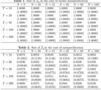
In this subsection, the wrong model is used. Table 1 presents the empirical size at 5% signi…cance level corresponding to the critical value 1.645 (one-sided test). In this case, the true model is Model 2 but we wrongly use the statistic
Z ;hence, committing a deliberate misspeci…cation. The tests have extremely severe size distortions, all equal to 1. This means that despite that the null hypothesis is true, we will wrongly reject it all the time. The same conclusion is reached when we use the tests whereT is assumed …nite.
[Table 1 here]
Table 2 shows the reverse situation. The data is generated by Model 1 but we employ on purpose the wrong statisticZ :For the case whereT is assumed asymptotic, the size of the test is very close to the nominal value 0.05 for samples withT >25:As expected, asTandNget larger butNis not too large relatively toT, the test becomes less distorted. This is due to the relative rate condition:
N=T !0 whenT; N ! 1. ForT assumed …xed, the size does not deteriorate even whenN is larger than T;as expected.
[Table 2 here]
3.2
Model misspeci…cations in a mixed stationary panel
In thissubsection, we investigate the mixed stationary panel data where there areM (M < N) cross-sections, which are from Model 1, while the remaining (N M) cross-sections are generated by Model 2. We apply the panel test statisticsZ andZ in turn to a mixed stationary panel data to evaluate their performances.
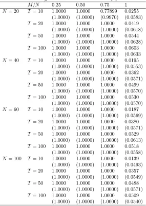
We have misspeci…cation whether we apply Z or Z statistic in a mixed stationary panel data. Table 3 and Table 4 report the simulation results about the size of Z and Z respectively. Di¤erent proportions of each models in a panel are examined.
The results in Table 3, where we use Z statistic, reveal that most results have large size distortion whenM=N <1under both assumptions of T asymp-totic andT …xed. We …nd that there is a tendency for the size to improve when the proportion of level stationary models increases. At the extreme point when
M=N = 1, that is, all the cross-sections are generated by Model 1, there is no misspeci…cation problem and the sizes are close to the nominal 0.05 as expected. Similar results are obtained whenT is assumed …xed.
[Table 3 here]
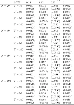
In Table 4, where we use Z statistic, we …nd that the calculated sizes are very close to the nominal one for any combination ofT,N and M=N whenT
[Table 4 here]
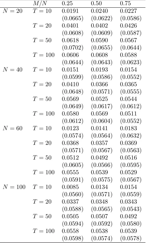
3.2.1 The correct statistic for mixed panel data
Table 5 gives the sizes in a mixed panel data where the correct statistic in-corporating the information about the mixture is used. The sizes for bothT
asymptotic and T …xed are very close to the nominal one. The statistic forT
asymptotic is slightly undersized whenT is very small ( 10). [Table 5 here]
4
Conclusion
This paper extends the panel stationarity test proposed by Hadri (2000) and Hadri and Larsson (2005) to the more realistic case of model misspeci…cation. The investigations are based on the assumptions ofT asymptotic and T …xed. Monte Carlo simulations are used to analyze the e¤ects of misspeci…cations. The results suggest that using the statistic corresponding to Model 2 is very robust to misspeci…cation. The statistic under the assumption of T …xed performs better than the statistic where T is assumed asymptotic particularly when T
Appendix
Proof. of equation (10).We recall that (cf. Hadri (2000)):
b i=T 2 T
X
t=1
Sit2=b2i ! Z
V (r)2dr as T ! 1
and
b i=T 2 T
X
t=1
Sit2=b2i ! Z
V (r)2drasT ! 1
Hence, for Model 1
E(b i)!E Z
V (r)2dr= ; V(b i)!V ar(
Z
V (r)2dr) = 2
and for Model 2
E(b i)!E Z
V (r)2dr= ; V(b i)!V ar(
Z
V (r)2dr) = 2:
The values of the above moments are given by (7) and (8) forT asymptotic and
T …xed respectively.
Calculations of the mean and variance ofLMd andLMd are as follows. For Model 1, since
d
LM = 1
M(
M
X
i=1 1
T2( PT
t=1Sit2)
b2i";1
) = 1
M
M
X
i=1
(b i);
therefore
E[LMd ] = 1
M
M
X
i=1
E(b i) = ;
and
V ar(LMd ) = V ar( 1
M(
M
X
i=1
b i)
= 1
M2
M
X
i=1
V ar(b i)
= 1
M
2:
For Model 2, we have
d
LM = 1
N M(
N
X
i=M+1 1
T2( PT
t=1Sit2)
b2i";1
)
= 1
N M
N
X
i=M+1
so we can …nd
E(LMd ) = 1
N M
N
X
i=M+1
E(ci) =
and
V ar(LMd ) = V ar( 1
N M
N
X
i=M+1
b i)
= 1 (N M)2
N
X
i=M+1
V ar(b i)
= 1
N M
2
Derivation of the mean and variance ofLMdm are as follows:
d
LMm=
M
N(LMd ) +
N M
N (LMd );
E[LMdm] =
M
N(E[LMd ]) +
N M
N (E[LMd ])
= M
N( ) +
N M
N ( )
= m
and
V ar[LMdm] = M
2
N2(V ar[LMd ]) +
(N M)2
N2 (V ar[LMd ])
= M
2
N2
1
M(
2) +(N M)2
N2
1
N M(
2)
= M
N2( 2
) +N M
N2 (
2 ) = 1 N 2 m:
Recall that asM ! 1andN M ! 1(while remains constant)
Z =
p
M(LMd )
!N(0;1)
and as
Z =
p
N M(LMd )
!N(0;1)
It follows that LMdm which is a weighted average of LMd and LMd has the following limiting distribution
Zm=
p
N(LMdm m)
m !
where
m =
M + (N M)
N = + (1 )
2
m =
M 2 + (N M) 2
N =
2
Table 1. Size ofZ in the case of model misspeci…cation
N = 5 N = 10 N = 15 N= 25 N= 50 N= 100
T = 10 1:0000 1:0000 1:0000 1:0000 1:0000 1:0000
(1:0000) (1:0000) (1:0000) (1:0000) (1:0000) (1:0000)
T = 20 1:0000 1:0000 1:0000 1:0000 1:0000 1:0000
(1:0000) (1:0000) (1:0000) (1:0000) (1:0000) (1:0000)
T = 50 1:0000 1:0000 1:0000 1:0000 1:0000 1:0000
(1:0000) (1:0000) (1:0000) (1:0000) (1:0000) (1:0000)
T = 100 1:0000 1:0000 1:0000 1:0000 1:0000 1:0000 (1:0000) (1:0000) (1:0000) (1:0000) (1:0000) (1:0000)
T = 200 1:0000 1:0000 1:0000 1:0000 1:0000 1:0000 (1:0000) (1:0000) (1:0000) (1:0000) (1:0000) (1:0000)
Table 2. Size ofZ in the case of misspeci…cation
N = 5 N = 10 N = 15 N= 25 N= 50 N= 100
T = 10 0:0079 0:0052 0:0049 0:0023 0:0012 0:0002
(0:1021) (0:1145) (0:1146) (0:1244) (0:1256) (0:1290)
T = 20 0:0336 0:0322 0:0313 0:0223 0:0226 0:0193
(0:0848) (0:0922) (0:0962) (0:0911) (0:0917) (0:0916)
T = 50 0:0572 0:0496 0:0502 0:0503 0:0427 0:0362
(0:0746) (0:0699) (0:0775) (0:0794) (0:0733) (0:0615)
T = 100 0:0618 0:0556 0:0551 0:0545 0:0547 0:0500 (0:0687) (0:0639) (0:0676) (0:0682) (0:0673) (0:0644)
Table 3 Size ofZ in model of mixed stationary panel series
M=N 0:25 0:50 0:75 1
N = 20 T = 10 1:0000 1:0000 0:77899 0:0255 (1:0000) (1:0000) (0:9970) (0:0583)
T = 20 1:0000 1:0000 1:0000 0:0419
(1:0000) (1:0000) (1:0000) (0:0618)
T = 50 1:0000 1:0000 1:0000 0:0544
(1:0000) (1:0000) (1:0000) (0:0628)
T = 100 1:0000 1:0000 1:0000 0:0603 (1:0000) (1:0000) (1:0000) (0:0633
N = 40 T = 10 1:0000 1:0000 1:0000 0:0195
(1:0000) (1:0000) (1:0000) (0:0553)
T = 20 1:0000 1:0000 1:0000 0:0362
(1:0000) (1:0000) (1:0000) (0:0571)
T = 50 1:0000 1:0000 1:0000 0:0499
(1:0000) (1:0000) (1:0000) (0:0570)
T = 100 1:0000 1:0000 1:0000 0:0530 (1:0000) (1:0000) (1:0000) (0:0570)
N = 60 T = 10 1:0000 1:0000 1:0000 0:0187
(1:0000) (1:0000) (1:0000) (0:0569)
T = 20 1:0000 1:0000 1:0000 0:0380
(1:0000) (1:0000) (1:0000) (0:0571)
T = 50 1:0000 1:0000 1:0000 0:0529
(1:0000) (1:0000) (1:0000) (0:0613)
T = 100 1:0000 1:0000 1:0000 0:0518 (1:0000) (1:0000) (1:0000) (0:0558)
N = 100 T = 10 1:0000 1:0000 1:0000 0:0139 (1:0000) (1:0000) (1:0000) (0:0493)
T = 20 1:0000 1:0000 1:0000 0:0357
(1:0000) (1:0000) (1:0000) (0:0549)
T = 50 1:0000 1:0000 1:0000 0:0488
(1:0000) (1:0000) (1:0000) (0:0571)
Table 4. Size ofZ in model of mixed stationary panel series
M=N 0:25 0:50 0:75 1
N = 20 T = 10 0:0031 0:0034 0:0034 0:0032
(0:0548) (0:0558) (0:0595) (0:0564)
T = 20 0:0252 0:0250 0:0285 0:0281
(0:0579) (0:0567) (0:0567) (0:0583)
T = 50 0:0501 0:0451 0:0488 0:0498
(0:0620) (0:0582) (0:0596) (0:0611)
T = 100 0:0537 0:0530 0:0536 0:0542 (0:0604) (0:0585) (0:0597) (0:0596)
N = 40 T = 10 0:0013 0:0014 0:0016 0:0019
(0:0575) (0:0563) (0:0550) (0:0563)
T = 20 0:0200 0:0198 0:0223 0:0198
(0:0556) (0:0538) (0:0573) (0:0583)
T = 50 0:0445 0:0462 0:0453 0:0458
(0:0555) (0:0594) (0:0590) (0:0573)
T = 100 0:0471 0:0511 0:0511 0:0510 (0:0527) (0:0576) (0:0580) (0:0567)
N = 60 T = 10 0:0010 0:0018 0:0010 0:0010
(0:0537) (0:0521) (0:0518) (0:0537)
T = 20 0:0217 0:0197 0:0203 0:0208
(0:0541) (0:0551) (0:0563) (0:0578)
T = 50 0:0432 0:0414 0:0436 0:0415
(0:0577) (0:0542) (0:0575) (0:0537)
T = 100 0:0521 0:0486 0:0498 0:0493 (0:0573) (0:0548) (0:0560) (0:0546)
N = 100 T = 10 0:0004 0:0003 0:0003 0:0005 (0:0518) (0:0496) (0:0543) (0:0515)
T = 20 0:0198 0:0183 0:0170 0:0166
(0:0575) (0:0551) (0:0556) (0:0526)
T = 50 0:0406 0:0428 0:0412 0:0421
(0:0544) (0:0561) (0:0548) (0:0564)
Table 5 Size ofZmin mixed stationary panel series
M=N 0:25 0:50 0:75
N = 20 T = 10 0:0191 0:0240 0:0227
(0:0665) (0:0622) (0:0586)
T = 20 0:0401 0:0402 0:0426
(0:0608) (0:0609) (0:0587)
T = 50 0:0618 0:0590 0:0567
(0:0702) (0:0655) (0:0644)
T = 100 0:0606 0:0608 0:0588 (0:0644) (0:0643) (0:0623)
N = 40 T = 10 0:0151 0:0193 0:0154
(0:0599) (0:0586) (0:0552)
T = 20 0:0410 0:0366 0:0365
(0:0648) (0:0571) (0:0555)
T = 50 0:0569 0:0525 0:0544
(0:0649) (0:0617) (0:0612)
T = 100 0:0580 0:0569 0:0511 (0:0612) (0:0604) (0:0552)
N = 60 T = 10 0:0123 0:0141 0:0183
(0:0574) (0:0564) (0:0632)
T = 20 0:0368 0:0357 0:0369
(0:0571) (0:0567) (0:0563)
T = 50 0:0512 0:0492 0:0516
(0:0605) (0:0566) (0:0595)
T = 100 0:0555 0:0539 0:0529 (0:0591) (0:0575) (0:0567)
N = 100 T = 10 0:0085 0:0134 0:0154 (0:0560) (0:0571) (0:0559)
T = 20 0:0337 0:0348 0:0343
(0:0588) (0:0565) (0:0543)
T = 50 0:0505 0:0507 0:0492
(0:0594) (0:0592) (0:0580)
References
[1] Abadir, K. M. (1993). OLS Bias in nonstationary autoregression. Econo-metric Theory 9,81-93.
[2] Abadir, K. M. and K. Hadri (2000). Is more information a good thing? Bias nonmonotonicity in stochastic di¤erence equations. Bulletin of Economic Research 52, 91-100.
[3] Baltagi, B. H.(2001).Econometric Analysis of Panel Data. Chichester, Wi-ley.
[4] Baltagi, B. H. and C. Kao (2000). Nonstationary panels, cointegration in panels and dynamic panels: A survey.Advances in Econometrics 15, 7-51. [5] Banerjee, A. (1999). Panel data unit roots and cointegration: An overview.
Oxford Bulletin of Economics and Statistics Special issue, 607-29.
[6] Breitung, J. and W. Meyer (1994). Testing for unit roots in panel data: Are wages on di¤erent bargaining levels cointegrated? Applied Economics
26, 353-61.
[7] Breitung, J. and Pesaran, M. H. (2005). Unit roots and cointegration in panels.Cambridge Working Papers in Economics 0535.
[8] Carrion-i-Silvestre, J. L., T. Del Barrio and E. López-Bazo (2005). Breaking the panels: An application to the GDP per capita. Econometrics Journal
8, 159-175.
[9] Culver, S. E., and Papell, D. H., (1997). Is there a unit root in the in‡ation rate? Evidence from sequential break and panel data models, Journal of Applied Econometrics, 12, 4, 435-444.
[10] Hadri, K (2000). Testing for stationarity in heterogeneous panel data.
Econometrics Journal, 3, 148-161.
[11] Hadri, K. and G. D. A. Phillips (1999). The accuracy of the higher order bias approximation for the 2SLS estimator.Economic Letters 62, 167-74. [12] Hadri, K and R. Larsson, (2005). Testing for stationarity in heterogeneous
panel data where the time dimension is …nite. Econometrics Journal, 8, 55-69.
[13] Hadri, K. and Rao, Y. (2007). Panel stationarity test with structural breaks.
Oxford Bulletin of Economics and Statistics. Forthcoming.
[15] Kwiatkowski, D., Phillips, P.C.B., Schmidt, P. and Shin, Y., (1992). Testing the null of stationarity against the alternative of a unit root: How sure are we that economic time series have a unit root? Journal of Econometrics
54 (1-3), 159-178.
[16] Levin, A., C. F. Lin and C. S. J. Chu (2002). Unit root tests in panel data: Asymptotics and …nite-sample properties. Journal of Econometrics
108, 1-24.
[17] Maddala, G. S. and S. Wu (1999). A comparative study of unit root tests with panel data and a new simple test. Oxford Bulletin of Economics and Statistics 61, 631-52.
[18] Nabeya, S. and K. Tanaka (1988). Asymptotic theory of a test for the constancy of regression coe¢ cients against the random walk alternative.
Annals of Statistics 16, 218-35.
[19] Quah, D. (1994). Exploiting cross section variation for unit root inference in dynamic data.Economics Letters 44, 9-19.
[20] O’Connell P. G. J. (1998). The overvaluation of purchasing power parity.
Journal of International Economics,44, 1-19.
[21] Oh., K.Y. (1996) .Purchasing power parity and unit root tests using panel data. Journal of International Money and Finance, 15, 405-418.
[22] Papell, D.H. (1997). Searching for stationarity: purchasing power parity under the current ‡oat. Journal of International Economics 43,313-332 [23] Papell, D.H. (2002). The great appreciation, the great depreciation and the
purchasing power parity hypothesis. Journal of International Economics
57,51-82
[24] Phillips, P.C.B.and Moon, H.R. (1999). Linear regression limit theory for nonstationary panel data. Econometrica67, 1057-1111.
[25] Wu, S. and Wu, J. L. (2001). Is purchasing power parity overvalued? Jour-nal of Money, Credit and Banking 33,804-812.