This is a repository copy of Joint target tracking and classification with particle filtering and mixture Kalman filtering using kinematic radar information.
White Rose Research Online URL for this paper: http://eprints.whiterose.ac.uk/82261/
Version: Submitted Version
Article:
Angelova, D. and Mihaylova, L. (2006) Joint target tracking and classification with particle filtering and mixture Kalman filtering using kinematic radar information. Digital Signal Processing , 16 (2). 180 - 204. ISSN 1051-2004
https://doi.org/10.1016/j.dsp.2005.04.007
Reuse
Unless indicated otherwise, fulltext items are protected by copyright with all rights reserved. The copyright exception in section 29 of the Copyright, Designs and Patents Act 1988 allows the making of a single copy solely for the purpose of non-commercial research or private study within the limits of fair dealing. The publisher or other rights-holder may allow further reproduction and re-use of this version - refer to the White Rose Research Online record for this item. Where records identify the publisher as the copyright holder, users can verify any specific terms of use on the publisher’s website.
Takedown
If you consider content in White Rose Research Online to be in breach of UK law, please notify us by
Joint Target Tracking and Classification with Particle
Filtering and Mixture Kalman Filtering
Using Kinematic Radar Information
Donka Angelova
a, Lyudmila Mihaylova
∗
,b,
aCentral Laboratory for Parallel Processing, Bulgarian Academy of Sciences, 25A Acad.
G. Bonchev St, 1113 Sofia, Bulgaria
bDepartment of Electrical and Electronic Engineering, University of Bristol, Merchant
Venturers Building, Woodland Road, Bristol BS8 1UB, UK
Abstract
This paper considers the problem of joint maneuvering target tracking and classification. Based on recently proposed Monte Carlo techniques, a multiple model (MM) particle filter and a mixture Kalman filter (MKF) are designed for two-class identification of air targets: commercial and military aircraft. The classification task is carried out by processing radar measurements only, no class (feature) measurements are used. A speed likelihood function for each class is defined using a prior information about speed constraints. Class-dependent speed likelihoods are calculated through the state estimates of each class-dependent tracker. They are combined with the kinematic measurement likelihoods in order to improve the classification process. The two designed estimators are compared and evaluated over rather complex target scenarios. The results demonstrate the usefulness of the proposed scheme for the incorporation of additional speed information. Both filters illustrate the opportunity of the particle filtering and mixture Kalman filtering to incorporate constraints in a natu-ral way, providing reliable tracking and correct classification. Future observations contain valuable information about the current state of the dynamic systems. In the framework of the MKF, an algorithm for delayed estimation is designed for improving the current modal state estimate. It is used as an additional, more reliable information in resolving compli-cated classification situations.
Key Words: Joint tracking and classification, particle filtering, mixture Kalman
fil-tering, multiple models, maneuvering target tracking
∗ Corresponding author
Email addresses:[email protected](Donka Angelova),
1 Introduction
Recently there has been great interest in the problem of joint target tracking and classification. It is due to the fact that the simultaneous implementation of these two important tasks in the surveillance systems facilitates the situation assessment, resource allocation and decision-making. Classification (or identification) usually includes target allegiance determination and/or target profile assessment such as
ve-hicle, ship or aircraft type. Target class information could be obtained from an elec-tronic support measure (ESM) sensor, friend-and-foe identification system, high
resolution radar or other identity sensors. It can be inferred from a tracker, using kinematic measurements only or in combination with identity sensors. On the other hand, target type knowledge applied to the tracker can improve the tracking per-formance by the possibility of selecting appropriate target models. Classification information can assist in correct data association and false tracks elimination in multiple target tracking systems. The notion of joint tracking and classification
(JTC) was introduced by Challa and Pulford in [1].
Several methods such as Bayesian [1–4], Dempster-Shafer [5,6] methods and fuzzy
set theory [7] have been applied to solve different identification problems.
Compar-ative studies of these techniques have been published in the specialized literature [5]. The inferences for their advantages and disadvantages are usually conflicting. They are highly dependent on the particularities of the problem of interest. In ad-dition, the combination of elements from different approaches often leads to inter-esting results [6]. We focus here on the Bayesian methodology because it offers a theoretically valid framework for overcoming the uncertainties of the JTC. From a Bayesian point of view the problem is reduced to reconstructing of the joint poste-rior probability density function of the target state and class over time. However, the optimal solution is infeasible in practice due to the prohibitively time-consuming computations.
are more easily implementable for systems of high dimension.
Particle filters [9,10] are sequential Monte Carlo methods based on “particle” (sam-ple) representation of probability densities. Multiple particles of the variables of interest are generated, each associated with a weight which characterizes the qual-ity of a specific particle. An estimate of the variable of interest is obtained by the weighted sum of particles. In the grid-based algorithms the grid points are chosen by the designer, whereas in the particle filter the particles are randomly generated according to the model of the dynamic system and then naturally follow the state. Sequential Monte Carlo algorithms are particularly suitable for classification pur-poses. The highly non-linear relationships between state and class measurements and non-Gaussian noise processes can be easily processed by the particle filtering technique. Moreover, flight envelope constraints, especially useful for this task, can be incorporated into the filtering algorithm in a natural and consistent way [11].
One of the first papers where particle filtering techniques are applied to tracking and identification is [12] addressing two closely spaced objects in clutter. Later other feasible implementations are reported [4,13]. Automatic target recognition and tracking of multiple targets with particle filters is proposed in [14] by the in-clusion of radar cross section measurements into the measurement vector.
The main idea of using sequential Monte Carlo filtering for JTC consists of filling the state and class space with particles and then running the filtering procedure. Since the probability of switching between classes is zero, all the particles might eventually cluster around one class [4]. This is a crucial shortcoming in some cases of classification. This could happen in many practical situations, for instance, when the classification decision is not yet been taken, and all particles might be clustered around one of the classes. Therefore, the number of particles for each class should remain constant. To overcome this drawback, Gordon, Maskell and Kirubarajan [4] suggest the following algorithm for JTC: a bank of independent filters, covering the state and feature space are run in parallel with each filter matched to a differ-ent target class. The class-conditioned independdiffer-ent filters stay in position “alert” and the filtering system can “change its mind” regarding the class identification if changes in the target behavior occur. An example of a successful application of this approach to littoral tracking with classification is proposed in [13].
The latent variable can take values over a given set of possible values depending on the acceleration range. Given the indicator variable, a set of Kalman filters realize on-line filtering based on dynamic linear models. In such a way a multiple model structure is implemented together with Monte Carlo sampling in the space of the latent variables, instead of in the space of the state variables. The paper represents a further development and generalization of the results reported in [19,20]. Two air target classes are considered: commercial aircraft (slowly maneuverable, mainly straight line) and military aircraft (highly maneuverable turns are possible). The features of the proposed algorithms include the following:
• for each target class a separate filter is designed. These filters operate in parallel,
covering the class space.
• each class-dependent filter represents a switching multiple model filtering
proce-dure, covering the class-dependent kinematic state space.
• two kinds of constraints are imposed on the target kinematic parameters: on the
acceleration and on the speed. Two speed likelihood functions are defined based
on a prior information about the speed constraints of each class. At every filtering step, the estimated speed from each class-dependent filter is used to calculate class-dependent speed likelihoods. These speed likelihoods are combined with kinematic likelihoods in order to improve the process of classification.
• Future observations contain valuable information about the current target state
[21] and a delayed sampling scheme applied to fading communication channels was shown to improve the estimation accuracy. The JTC solution can achieve better performance when such a delayed estimation of the current maneuvering
mode state is incorporated into the MKF structure. It is used as an additional,
more reliable information in resolving ambiguous classification situations.
The novelty of the present paper relies on combining the multiple model (MM) approach with the particle filtering and mixture Kalman filtering for JTC purposes, the manner of imposing the speed constraints on target behavior and the use of delayed estimation for classification. Although we consider only two classes, the generalization for more target classes is straightforward.
The remaining part of the paper is organized as follows. Section 2 summarizes the Bayesian formulation of the JTC problem according to [4,13,22]. Section 3 presents the developed MM particle filter, MKF, and delayed-pilot MKF using speed and acceleration constraints. Simulation results are given in Section 5. Finally, Section 6 contains the conclusions.
2 Bayesian joint target tracking and classification
xk=F (mk)xk−1+G(mk)uk(mk) +B(mk)wk, (1)
zk=h(mk,xk) +D(mk)vk, k = 1,2, . . . , (2)
where xk ∈ Rnx is the base (continuous) state vector with transition matrix
F, zk ∈ Rnz specifies the measurement vector with measurement function h,
uk ∈ Rnu represents a known control input and k is a discrete time. The
in-put noise process wk and the measurement noise vk are independent identically
distributed Gaussian processes having characteristics wk ∼ N(0,Q) and vk ∼
N(0,R), respectively. The modal (discrete) state mk, characterizing the
differ-ent system modes (regimes), can take values over a finite set S, i.e. mk ∈ S ,
{1, 2, . . . , s}. We assume that mk is evolving according to a time-homogeneous first-order Markov chain with transition probabilities
πij ,P r{mk =j |mk−1 =i}, (i, j ∈S) (3)
and initial probability distribution P0(i) , P r{m0 =i} for i ∈ S, such that
P0(i) ≥ 0, and Psi=1P0(i) = 1. Next we suppose that the target belongs to one
of M classes c ∈ C where C = {c1, c2, . . . , cM}represents the set of the target
classes. Generally, the number of the discrete statess=s(c), the initial probability
distribution Pc
0(i)and the transition probability matrix π(c) =
h
πc ij
i
, i, j ∈ S(c) are different for each target class. Note that the joint state and class is time varying with respect to the state and time invariant with respect to the class [4].
Denote withωk ,{zk,yk}the set of kinematiczkand class (feature)yk
measure-ments obtained at time instantk. Then Ωk = nZk,Yko specifies the cumulative
set of kinematicZk = {z1,z2, . . . ,zk}and featureYk = {y1,y2, . . . ,yk}
mea-surements, available up to timek.
The goal of the joint tracking and classification task is to estimate simultaneously
the base statexk, the modal statemk and the posterior classification probabilities
P ³c|Ωk´, c ∈Cbased on all available measurement informationΩk.
If we can construct the posterior joint state-mode-class probability density
func-tion (pdf) p³xk, mk, c|Ωk ´
, then the posterior classification probabilities can be
obtained by marginalization overxkandmk:
P ³c|Ωk´= X mk∈S(c)
Z
xk∈Rnxp ³
xk, mk, c|Ωk ´
dxk. (4)
Suppose that we know the posterior joint state-mode-class pdfp³xk−1, mk−1, c |Ωk−1
´
at time instantk−1. According to the Bayesian framework,p³xk, mk, c |Ωk
´ can
be computed recursively from p³xk−1, mk−1, c |Ωk−1
´
in two steps – prediction and measurement update [4,13].
The predicted state-mode-class pdf p³xk, mk, c|Ωk−1
´
equation
p³xk, mk, c|Ωk−1 ´
= (5)
X
mk−1∈S(c)
Z
xk
−1∈Rnx
p³xk, mk|xk−1, mk−1, c,Ωk−1 ´
×p³xk−1, mk−1, c|Ωk−1 ´
dxk−1,
where the state prediction pdfp³xk, mk|xk−1, mk−1, c,Ωk−1
´
is obtained from the state transition equation (1)
p³xk, mk|xk−1, mk−1, c,Ωk−1 ´
∝
∝ X
mk∈S(c)
p³xk|mk,xk−1, mk−1, c,Ωk−1 ´
×P³mk|xk−1, mk−1, c,Ωk−1 ´
=
= X
mk∈S(c)
p³xk|mk,xk−1, mk−1, c,Ωk−1
´ X
mk−1∈S(c) πmkc
−1mkP
³
mk−1|xk−1, c,Ωk−1 ´
.
(6)
The form of the conditional pdf of the measurements
p(ωk|xk, mk, c) = λ{xk,mk,c}(ωk) (7)
is usually known. This is the likelihood of the joint state and feature and has a key role in the classification algorithm. In our case we do not have feature
measure-ments yk, k = 1,2, . . . . The speed estimates from theM classes, together with
speed envelope constraints, whose shapes are given in Section 3.3, form a virtual
“feature measurement” set{Yk}.
When the measurementωkarrives, the update step can be completed
p³xk, mk, c|Ωk ´
= λ{xk,mk,c}(ωk)p ³
xk, mk, c |Ωk−1 ´
p³ωk|Ωk−1
´ , (8)
where
p³ωk |Ωk−1 ´
= X
c∈C
X
mk∈S(c) Z
xk∈Rnx p(ωk |xk, mk, c)p ³
xk, mk, c |Ωk−1 ´
dxk.
The recursion (5)-(8) begins with the prior densityP {x0, m0, c}, assumed known,
wherex0 ∈Rnx, c ∈C,m0 ∈S(c). Using Bayes’ theorem, the posterior
probabil-ity of the discrete statemkfor classcis expressed by
P ³mk |xk, c,Ωk ´
= (9)
1
αk
λ{xk,mk,c}(ωk)× X
mk−1∈S(c)
Z
xk
−1∈Rnx
πmkc −1mkP
³
mk−1 |xk−1, c,Ωk−1 ´
whereαkis a normalizing constant. Eq. (9) is substituted into (6) in order to predict
the state pdf at timek+ 1.
Then the target classification probability is calculated by the equation
P ³c|Ωk´= P
mk∈S(c) R
xk∈Rnx p ³
ωk | xk, mk, c,Ωk−1 ´
p(xk, mk, c |Ωk−1)dxk
p³ωk |Ωk−1 o
(10)
that can be expressed as
P³c|Ωk´= p ³
ωk| c,Ωk−1 ´
P³c|Ωk−1´
PM
i=1p ³
ωk| ci,Ωk−1 ´
P³ci |Ωk−1 ´
with an initial prior target classification probabilityP0(c),Pc∈CP0(c) = 1.
The state estimatexˆckfor each classc
ˆ
xck = X
mk∈S(c) Z
xk∈Rnx xkp ³
xk, mk, c |Ωk ´
dxk,c ∈C (11)
takes part in the calculation of the combined state estimate
ˆ
xk= X
c∈C
ˆ
xckP³c|Ωk´. (12)
It is obvious from (5)-(12) that the estimates, needed for each class, can be calcu-lated independently from the other classes. Therefore, the JTC task can be
accom-plished by the simultaneous work ofM independent filters.
3 Maneuvering target tracking and classification
3.1 Maneuvering target model
The two-dimensional target dynamics are given by
xk=F xk−1+G(uk+wk), k= 1,2, . . . , (13)
where the state vectorx = (x,x, y,˙ y˙)′ contains target positions and velocities in
the horizontal (Oxy) Cartesian coordinate frame. The control input vector u =
w = (wx, wy)′ models perturbations in the accelerations. The transition matrices
F andGare [23]
F =diag(F1,F1), G=diag(g1,g1),
where
F1 =
1 T
0 1
, for g1 =
µ T2
2 T
¶′
,
T is the sampling interval andB = G. The target is assumed to belong to one of
two classes (M = 2), representing either a lower speed commercial aircraft with
limited maneuvering capability (c1) or a highly maneuvering military aircraft (c2)
[1]. The flight envelope information comprises speed and acceleration constrains,
characterizing each class. The speed v=√x˙2 + ˙y2 of each class is limited
respec-tively to the interval:
{c1 :v∈(100,300)} [m/s] and{c2 :v∈(150,650)} [m/s].
The range of the speed overlap section is [150,300] [m/s]. The control inputs are
restricted to the following sets of accelerations:
{c1 :u∈(0,+2g,−2g)} [m/s2] and{c2 :u∈(0,+5g,−5g)} [m/s2],
whereg = 9.81 [m/s2]is the acceleration due to gravity. The acceleration process
ukis a Markov chain with five states (modes)s(c1) =s(c2) = 5[24]:
1. ax = 0, ay = 0, 2. ax =A, ay =A, 3. ax=A, ay =−A,
4. ax =−A, ay =A, 5. ax =−A, ay =−A, (14)
whereA= 2gstands for classc1target andA= 5g refers to the classc2(as shown
on Fig. 1 (a)).
The initial probabilities of the Markov chain are selected equal for the two classes
as follows:P0(1) = 0.6,P0(i) = 0.1, i = 2, . . . ,5. The matrix π(c)of transition
probabilities πc
ij, i, j ∈ S is assumed of the same form for both types of targets:
pij = 0.7 for i = j; p1j = 0.075 for j = 2, . . . ,5; pi1 = 0.15 for i =
2, . . . ,5; pij = 0.05 forj 6=i, i, j = 2, . . . ,5.
The process noise is Gaussian,w ∼ N(0,Q),Q=diag(σ2
wx, σwy2 ), having
differ-ent standard deviations for each mode and class:
{c1 :σw1 = 5.5; σwj = 7.5 [m/s2], j = 2, . . . ,5}and
{c2 :σw1 = 7.5, σwj = 17.5 [m/s2], j = 2, . . . ,5},
3.2 Measurement model
The measurement model at timek is described by
zk =h(xk) +vk, (15)
with
h(xk) = Ã
q
x2
k+y2k,arctan
xk
yk !′
, (16)
where the measurement vectorz = (D, β)′ consists of the distanceDto the target
and bearingβ, measured by the radar. The measurement error vectorv∼ N(0,R)
is assumed to be independent from w. The measurement noise covariance matrix
for the particle filter has the formR = diag(σ2
D, σβ2). The measurement function
h(x)is highly nonlinear and can be easily processed by the particle filter.
The MKF algorithm, however, works with linear state and measurement equations. For the purposes of the MKF design, a measurement conversion is performed from
polar (D , β) to Cartesian (x , y) coordinates: z = (Dcos(β), Dsin(β))′. Thus,
the measurement equation becomes linear with anz×nx measurement matrixH,
where all elements are zeros, except forH11 = H23 = 1. The components of the
corresponding measurement noise covariance matrixRare
R11 =σD2 sin
2(β) +D2σ2
βcos
2(β); R
22=σ2Dcos
2(β) +D2σ2
βsin
2(β);
R12 = (σD2 −D2σβ2) sin(β) cos(β); R21 =R12.
The following sensor parameters are selected in the simulations:σD = 100.0 [m]
σβ = 0.15 [deg]. The sampling interval isT = 5s.
3.3 Speed constraints
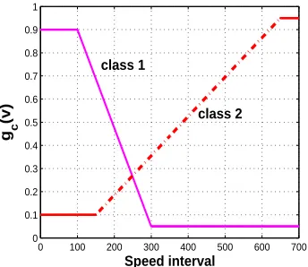
Acceleration constraints are imposed on the filter operation by the use of an appro-priate control input in the target model. The speed constraints are enforced through the speed likelihood functions. They are constructed based on the speed envelope information (3.1). Such constraints are incorporated into other approaches for deci-sion making [25]. We define the following speed likelihood functions, respectively for each class
g1(vck1) =
0.9, if vc1
k ≤100 [m/s]
0.9−κ1(vkc1 −100), if(100<v
c1
k ≤300 [m/s])
0.05 if vc1
and
g2(vck2) =
0.1, if vc2
k ≤150 [m/s]
0.1 +κ2(vkc2 −150), if(150<v
c2
k ≤650 [m/s])
0.95, if vc2
k >650 [m/s]
whereκ1 = 0.7/200andκ2 = 0.85/500. Fig. 1 (b) illustrates the evolution of the
likelihoods as a function of the speed.
−60 −40 −20 0 20 40 60
−60 −40 −20 0 20 40 60
acceleration interval for a x [m/s
2]
acceleration interval for a
y [m/s 2 ] Class c 1 Class c 2
m1= (0,0) m
2 = (2g,2g)
m
3 = (2g,−2g) m4 = (−2g,2g)
m5 = (−2g,−2g)
m 2 2 = (5g,5g)
m32 = (5g,−5g) m
4 2 = (−5g,5g)
m5 = (−5g,−5g)
0 100 200 300 400 500 600 700 0 0.1 0.2 0.3 0.4 0.5 0.6 0.7 0.8 0.9 1 Speed interval g c (v) class 1 class 2
Fig. 1. (a) Mode sets for two classes (b) Speed likelihood functions
According to the problem formulation, presented in Section 2, two class-dependent
filters work in parallel withNcnumber of particles for each class. At time step k
each filter gives a state estimate{xˆck, c= 1,2}. Let us assume that the estimated
speed from the previous time step,nˆvck−1, c = 1,2o, is a kind of “feature
measure-ment”.
The likelihoodλ{xk,mk,c}(ωk) =λ{xk,mk,c}({zk,yk})is factorized [4]
λ{xk,mk,c}({zk,yk}) =f(zk|xk, mk)gc(yck), (17)
where yck = ˆvck−1. Practically, the normalized speed likelihoods represent
speed-based class probabilities estimated by the filters. The posterior class probabilities
are modified by this additional speed information at every time stepk. The inclusion
of the speed likelihoods is done after some “warming-up” interval, comprising the filter initialization.
3.4 Multiple Model Particle Filter Algorithm
Within the JTC formulation problem as given in Section 2 a separate PF is designed for each target class. Assuming two classes of targets – commercial and military, we
[image:11.595.299.471.198.347.2]hybrid particles{x(ki), m(ki)} Nc
i=1, containing all the necessary information about the
target base state and modal state (mode). Each mode takes values from the setS(c).
The modes evolve in time according to a Markov chain with a transition probability matrix (3). The cloud of particles for every PF allows a sequential update of the pdfs (5)-(12) by two main stages: prediction and update. During the prediction each particle is modified according to the state model, including the addition of a random noise simulating the effect of the uncertainties on the state. Then in the update stage, each particle’s weight is re-evaluated based on the new sensor data. The resampling procedure deals with the elimination of particles with small weights and replicates the particles with higher weights.
[image:12.595.94.487.283.665.2]A detailed scheme of the proposed particle filter is given in Table 1.
Table 1: A Particle Filter for Joint Target Tracking and Classification
(1) Initialization, k= 0.
For class c= 1,2, . . . , M set class probabilities P¡
c|Ω0¢
=P0(c).
* For j= 1,2, . . . , Nc,
sample n
x(0j)∼p0(x0, c), m(0j)∼ {P0c(ℓ)} s(c) ℓ=1 o
and set initial weightsW0(j)= 1/Nc;
* End for j
End forc
Set k= 1.
(2) For c= 1,2, . . . , M (possibly in parallel) perform
* Prediction step
For j= 1,2, . . . , Nc
drawm(kj)from the set S(c) = 1,2, . . . s(c) with probability
P³m(kj)=i´∝πc
ℓ i, for ℓ=m
(j) k−1,
draw w(kj) ∼ N(0,Q(m(kj), c)),
calculate x(kj)=F x(kj−)1+Gu(m(kj), c) +Gw(kj),
whereu(m(kj), c)denotes the pair of accelerations from (14) corresponding tom(kj).
End forj
* Measurement processing step: on receipt of a measurementωk={zk, yk}:
For j = 1,2, . . . , Nc evaluate the weights
wheref(zk |x(kj)) =N(h(xk(j)),R) and gc(yck) =gc ¡
ˆ
vck−1 ¢
;
calculatep¡
ωk |c,Ωk−1 ¢
=PNc
j=1W
(j)
k and set L(c) =
PNc
j=1W
(j) k
End forj
normalize the weightsWk(j)=Wk(j)/PNc
j=1W
(j)
k ;
* Compute updated state estimate and posterior mode probabilities
ˆ
xck =PNc j=1x
(j)
k W
(j)
k ,
P¡
mk=ℓ|c,Ωk ¢
=E©
1 (mk=ℓ)|c,Ωk ª
∼
=PNc
j=11(m
(j)
k =ℓ)W
(j)
k , ℓ= 1,2, . . . , s(c),
where1(·)is an indicator function such that
1(mk =ℓ) = 1, if mk=ℓ and1(mk=ℓ) = 0 otherwise;
* Obtain a hard mode decision:
ˆ
mck= arg max
ℓ∈S(c)P ³
mk=ℓ|c,Ωk ´
∼
= arg max
ℓ∈S(c) Nc X
j=1
1(m(kj) =ℓ)Wk(j)
* Compute effective sample size: Nef f(c) = 1/PNcj=1
³
Wk(j)´2
End forc
(3) Output: Compute posterior class probabilities and combined output estimate
P¡
c|Ωk¢
= L(c)P(c|Ω
k−1)
PM
i=1L(ci)P(ci|Ω
k−1), c= 1,2, . . . , M
ˆ
xk=
PM
c=1P ¡
c|Ωk¢
ˆ
xck
(4) IfNef f(c)< Nthres, c= 1,2, . . . , M
resample with replacementNcparticles{x(kj), m
(j)
k };j= 1, . . . , Nc
from the set{x(kj), mk(j)};j= 1, . . . , Ncaccording to the weights;
setWk(j) = 1/Nc, j= 1, . . . , Nc
(5) Setk←−k+ 1and go to step 2.
3.5 The Mixture Kalman Filter Algorithm
The mixture Kalman filter (MKF) [26,27] is another sequential Monte Carlo esti-mation technique which has been successfully applied to different problems in tar-get tracking and digital communications (see e.g. [28,29]). It is essentially a bank of Kalman filters (KFs) run with the Monte Carlo sampling approach. The MKF is de-rived for state-space models in a special form, namely conditional dynamic linear
model (CDLM), conditional linear Gaussian model, or partially linear Gaussian model:
xk=Fλkxk−1+Gλkuλk +Gλkwk,
zk=Hλkxk+Vλkvk,
(18)
where wk ∼ N(0,Q) and vk ∼ N(0,Rc) are Gaussian distributed processes.
{λk} is a sequence of random indicator variables (called latent), independent of
wk, vk and the past state xs and measurement zs, s < k. The term conditional
justifies the characteristic of these models: they are linear for a given trajectory
of the indicatorλk. Then, the Monte Carlo sampling works in the space of latent
variables instead of in the space of the state variables. The matricesFλk,Gλk,Hλk
andVλk are known, assuming that λk is known. For simplicity, in the remaining
part of the paper we are omitting the subscript λk from the matrices of (18). The
indicator λk usually takes values from a preliminary known finite set. The MKF
relies on the conditional Gaussian property and uses a marginalization operation in order to improve the efficiency of the sequential Monte Carlo estimation technique.
Let Λk = {λ0, λ1, λ2, . . . , λk} be the set of indicator variables up to time
in-stant k. By recursively generating a set of properly weighted random samples
{(Λ(kj), W (j)
k )}Nj=1 to represent the pdf p(Λk|Ωk), the MKF approximates the state
pdfp(xk|Ωk)by a random mixture of Gaussian distributions [27]
N X
j=1
Wk(j)N(µk(j),Σk(j)), (19)
where µk(j) = µk(Λ(
j)
k ) and Σk(j) = Σk(Λ(
j)
k )are obtained by a KF, designed
with the system model (18). We denote by KFk(j) = {µk(j),Σ(
j)
k } the sufficient
statistics that characterize the posterior mean and covariance matrix of the statexk,
conditional on the set of accumulated observationsΩk and the indicator trajectory
Λ(kj). Then based on the set of samples{(Λ
(j) k−1, KF
(j) k−1, W
(j)
k−1)}Nj=1at the previous
time(k−1), the MKF produces a respective set of samples{(Λ(kj), KF
(j)
k , W
(j) k )}Nj=1
at the current timek. It is shown in [27] that the samples{(Λ(kj), KF
(j)
k , W
(j) k )}Nj=1
are indeed properly weighted with respect top(Λk|Ωk), if the samples
{(Λ(kj−)1, KF (j) k−1, W
(j)
k−1)}Nj=1 are properly weighted at time(k−1)with respect to
Table 2: The Mixture Kalman Filter for Joint Tracking and Classification
(1) Initialization,k= 0
For classc= 1,2, . . . , M set initial class probabilities P¡
c|Ω0¢
=P0(c).
* For j= 1, . . . , Nc,
sampleλ(0j) ∼ {Pc
0(λ)} s(c)
λ=1, whereP0c(λ)are the initial indicator
probabilities (for the target accelerations).
SetKF0(j)={µ0(λ(0j)),Σ0(λ(0j))}, whereµ0(λ( j)
0 ) = ˆµ0and
Σ0(λ(0j)) =Σ0are the mean and covariance of the initial statex0 ∼ N(ˆµ0,Σ0).
Set the initial weightsW0(j) = 1/Nc.
* end for j
End for classc
Set k= 1.
(2) For classc= 1,2, . . . , M complete
* Forj= 1, . . . , Nc,
• For eachλk=i, i∈S(c), compute
- KF prediction step
(µ(kj|)k−1)(i) =F µk(j−)1|k−1+Gu(λk =i, c),
(Σ(kj|)k−1)(i) =FΣ(j) k−1|k−1F
′+GQ(λ
k=i, c)G′,
(z(kj|)k−1)(i)=H(µ(j) k|k−1)(i),
(S(kj))(i)=H(Σ(j)
k|k−1)(i)H
′+V RV′.
Note thatjis a particle index, whilei= 1,2, . . . , s(c)is an index of the Kalman
filters with the different acceleration levels (14).
- on receipt of a measurementzkcalculate the likelihood
Lk,i(j) =f(zk|λk=i, KFk(−j)1)p(λk=i|λ(kj−)1), where
f(zk|λk=i, KF( j)
k−1) =N( (z (j)
k|k−1)(i),(S (j)
k )(i)), and
p(λk =i|λ( j)
k−1)is the prior transition probability of the indicator
• Sampleλ(kj) from a setS(c)with a probability, proportional toL(j)
k,i, i∈S(c);
sup-pose thatλ(kj)=ℓ, whereℓ∈S(c). Appendλ(j)
k toΛ
(j)
k−1and obtainΛ
(j)
k .
• perform the KF update step forλ(kj)=ℓ:
K(kj|k) = (Σ(kj|)k−1)(ℓ)(H)′[(S(j) k )(
µk(j|)k= (µk(j|)k−1)(ℓ)+K(j)
k|k[zk−(z (j) k|k−1)(ℓ)],
Σk(j|)k= (Σk(j|)k−1)(ℓ)−K(j) k|k(S
(j) k )(ℓ)K
(j)′
k|k,
• update the importance weights
Wk(j) =Wk(−j)1gc ¡
ˆ
vck−1 ¢ Ps(c)
i=1L (j) k,i
* end forj
SetL(c) =PNc
j=1W
(j)
k ;
Normalize the weightsWk(j) =Wk(j)/PNc
j=1W
(j) k
Compute the updated state estimate, posterior mode probabilities and hard mode
de-cision
ˆ
xck=PNc j=1µ
(j) k|kW
(j)
k , P(λck=i) =
PNc
j=11(λ (j)
k =i)W
(j)
k , i∈S(c)
ˆ
λck= arg max
i∈S(c)P(λ c k=i)
Compute the effective sample size: Nef f(c) = 1/PNcj=1 ³
Wk(j)´2
End for classc
(3) Output: Compute the posterior class probabilities and combined output estimate
(such as in the PF)
P¡
c|Ωk¢
= L(c)P(c|Ω
k−1)
PM
i=1L(ci)P(ci|Ω
k−1), c= 1,2, . . . , M
ˆ
xk=
PM
c=1P ¡
c|Ωk¢
ˆ
xck
(4) IfNef f(c)< Nthres, c= 1,2, . . . , M
resample with replacementNcparticles for each class:
λ(kj),µ(kj|)k,Σ(kj|k);j = 1, . . . , Ncaccording to the weights;
SetWk(j)= 1/Nc, j = 1, . . . , Nc
(5) Setk←−k+ 1and go to step 2.
Two MKFs are run in parallel, each of them according to the hypothesis:
respec-tively commercial or military aircraft. In our JTC problem the indicator variableλ
corresponds to the mode variablemfrom the previous sections. It takes values from
a finite discrete setS(c) , {1, 2, . . . , s(c)}and evolves according to a Markov
chain with transition probabilities (3).
At every time instant k, for each particle (j), j = 1, . . . , Nc, the MKF scheme
runs s(c) KF prediction steps, according to each λ ∈ S(c). The likelihood
They form a trial sampling distribution, according to which the newλkis selected. The MKF explores the predicted space in order to select the most likely value of
λ. Then the KF update step is accomplished only for the selected λk. In the
par-ticle filtering approach this procedure is realized in some chaotic (random) sense. This fact, together with the lack of the base state sampling, make the MK filtering more precise and more computationally efficient. However, the MKF application is limited to the CDLM. For that purpose the measurement equation (2) is linearized
through a coordinate conversion. It is assumed that the matricesF,G,H,V have
the same structure for two classes.
Notice that in both MM PF and MKF the updated state estimates and posterior mode probabilities are calculated before the resampling step, because resampling brings extra variation to the current samples ([30], [26], pp. 103).
3.6 Delayed-Pilot Mixture Kalman Filter
Since both types of aircraft can perform slow maneuvers, the recognition can only be achieved during the aircraft maneuvers with high speed and acceleration. In some cases it might take a rather long tracking time to distinguish the types. The estimated posterior mode probabilities can be used for a classification in compli-cated ambiguous situations. The reliability of the mode information can be further improved by using of a delayed mode estimation scheme. Since target maneuvers are usually modelled as a highly correlated acceleration process, the observations in the near future can provide a valuable information about the current mode state.
Recently, delayed estimation methods have been proposed for the purposes of mo-bile communications [29,21]. The idea of the delayed estimation consists in the
following. Based on the posterior distribution p(xk, λk | c,Ωk), an instantaneous
inference is made on the statexk and the indicator variable λk. If we use the next
measurements (ωk, . . . ,ωk+△,△ ≥ 0) with the distribution p(xk, λk | Ωk+△),
the current state and mode accuracy can be improved at the cost of delayed
es-timation at timek+△. Consequently, the aim of delayed estimation is to
gener-ate samples and weights nλ(kj), Wk(j)oNc
j=1 from the distribution p(Λk | Ω
k+△) at
timek+△. However, the algorithms for delayed estimation are more complicated.
Several schemes for delayed estimation are suggested in [29,21] in the context of mixture Kalman filtering: delayed-weight, delayed-sample sampling, delayed-pilot sampling. A highly effective delayed-sample sampling method is developed and
studied in [29]. It realizes a full exploration of the space of future states of△steps,
and generates samples of both the current state and the weights. Due to the need of marginalization over the future states, its computational complexity is exponential in terms of the delay.
exploring the entire space of future states, the delayed-pilot sampling generates a number of random pilot streams, each of which indicates what would happen in the future if the current state takes a particular value. The sampling distribution of the current state is then determined by the incremental importance weight associated
with each pilot stream. For each class c, at each time step k, the delayed-pilot
algorithm generatess(c)random pilot streams of the future states of△steps. Each
pilot stream starts with one of the possible values λi, i ∈ S and implements △
MKF steps. An incremental importance weight of this pilot stream is calculated
and assigned to λi. The aim is to utilize this information (that can forecast what
would happen in the future) for generating better samples of λ. A sample of the
current state is drawn proportionally to the incremental importance weight. This algorithm partially explores the space of future states. This fact explains why the pilot approximation introduces a bias, which is additionally corrected by the inverse of the pilot weights. A scheme of the delayed-pilot MKF [21], adapted to the JTC is given in Table 3. The algorithm starts with a conventional MKF, described in the previous section. The inclusion of the delayed estimation is done after the time
interval of15scans. Only the steps that are different are described for conciseness
(the other steps : initialization, output and resampling are the same as given in Table 2).
Suppose at time(k−1), a set of properly weighted samplesn³Λk(j−)1, KFk(j−)1, W
(j) k−1
´oNc
j=1
with respect top³Λk−1 |c,Ωk−1
´
are available. Then, as the new dataωk, . . . ,ωk+△
arrive, the following steps are implemented to obtainn³Λ(kj), KF
(j)
k , W
(j) k
´oNc
j=1for
[image:18.595.89.494.460.729.2]each classc:
Table 3: The delayed-pilot MKF for Joint Tracking and Classification
Forj = 1, . . . , Nc,
• for eachλk=i, i= 1,2, . . . , s(c) run a Kalman filter
KFk(j−)1 →zk→KF (j)
k,i ,N
h
µk ³
Λ(kj−)1, λk =i ´
,Σk ³
Λ(kj−)1, λk=i ´i
compute L(k,ij) =f(zk|Λ
(j)
k−1, λk =i, KF (j)
k−1)p(λk =i|Λ (j) k−1),
• for eachλ=i do the following:
for s=k+ 1, . . . , k+△, repeat
* LetΛ(si,j−1)=
h
Λ(kj−)1, λk =i, λk+1 =λ( i,j)
k+1, . . . , λs−1 =λ( i,j) s−1 i
for each λs =q, q ∈S(c), run a Kalman filter
KFs(−j)1,i →zs →KF( q,j)
s,i ,N
h
µs ³
Λ(si,j−1), λs =q ´
,Σs ³
Λ(si,j−1), λs =q ´i
* compute the sampling density
and draw a sampleλ(i,j)
s according to the sampling density;
ifλ(i,j)
s =ℓ, then setKF
(j)
s,i =KF
(ℓ,j) s,i
* compute the incremental importance weight
L(s,ij)= Ps(c)
q=1L (q,j) s,i
end fors
ρ(k,ij) =L (j) k,i
Qk+△
s=k+1L (j) s,i ,
end for eachλk =i,
˜
ρk,i(j) =ρk,i(j)/Ps(c) r=1ρ
(j)
k,r, i= 1,2, . . . , s(c),
use ρ˜(k,ij), i= 1,2, . . . , s(c) as the sampling distribution, draw a sample
λ(kj)and obtainΛ
(j)
k =
h
Λ(kj−)1, λ (j) k
i ,
if λ(kj)=ℓ, set KF
(j)
k =KF
(j) k,ℓ
• Compute the importance weights:
ifλ(kj) =ℓ, Wk(j) =Wk(−j)1L
(j)
k,ℓ
˜ ρ(k,ℓj) gc
³ ˆ
vck−1´,
calculate the auxiliary weight W˜k(j) =Wk(j)Qk+△
s=k+1L (j) s,ℓ,
end ofj
use the auxiliary weight to compute the posterior mode probabilities,
• Output: compute updated state estimate, posterior class probabilities and
combined output estimate according to the MKF scheme in Table 2.
• Resampling if the effective sample size is below a certain threshold.
• Setk ←−k+ 1and go to the beginning of the scheme.
Comment: The delayed-pilot MKF algorithm for JTC generates at time(k+△)a
weighted sample set³Λ(kj), Wk(j)´Nc
j=1, which is not properly weighted with respect
top(Λk |Ωkk+△). A better inference onλkat time(k+△)is done by the calculation
of auxiliary weights [21]. The auxiliary weights are used both for inference onλk
4 Simulation results
The performance of the implemented filters for JTC is evaluated by simulations over representative trajectories (shown on Figures 2 and 11) together with the radar location, indicated by a triangle. The target motion is generated without a process noise. The target trajectories were generated with a model ([31] Eqs. (57)–(60)) differing from the models used in the filters. The MM particle filter and the MKF using both speed and acceleration constraints with likelihood computed according to (17) are compared to filters without speed constraints, which likelihood is equal toλ{xk,mk,c} = fxk(zk|xk, mk, c). The performance of the designed delayed-pilot sampling algorithm for JTC is demonstrated on a specially selected target scenario (Fig. 22).
Measures of performance. Root-Mean Squared Errors (RMSEs) [32]: on position
(both coordinates combined) and speed (magnitude of the velocity vector), average
probability of correct class identification and average time per update are used
to evaluate the filters performance. The results presented below are based on 100
Monte Carlo runs. The PF hasNc = 3000particles per class, the MKF hasNc =
300particles per class, and the resampling threshold isNthresh =Nc/10. The prior
class probabilities are chosen to be equal:P0(1) =P0(2) = 0.5. The parameters of
the base state vector initial distributionx0 ∼ N (m0,P0)in the PF are selected as
follows: P0 =diag(1502 [m], 20.02 [m/s], 1502 [m], 20.02[m/s]);m
0 contains
the exact initial target states. The MKF initial parameters (mean and covarianceµˆ0
Σ0 of the initial statex0 ∼ N( ˆµ0,Σ0)) are obtained by a two-point differencing
technique [23] (p. 253), andV =I. The sampling period isT = 5 [s].
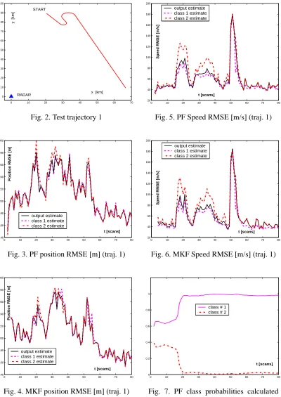
Test trajectory 1. The simulated target path is shown in Figure 2. The target
accom-plishes two turn maneuvers with normal accelerations 2g [m/s2] and 1g [m/s2],
respectively with a constant speed of v = 200 [m/s]. Then a maneuver is
per-formed with a longitudinal acceleration of2g [m/s2]in the frame of 3 scans. The
speed increases up to500 [m/s]. Practically, these maneuvers are typical for targets
of the first class. If the speed constraints are not imposed, the target is classified as belonging to the first class as it can be seen from Figure 7. But it actually belongs to the second class which is correctly distinguished by the speed likelihoods (Figure
9) when the target speed exceeds the value of300 [m/s](during the maneuver with
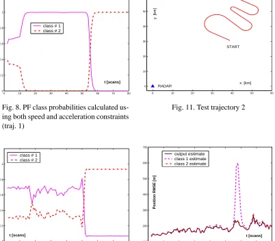
Test trajectory 2. The target performs four turn maneuvers (Figure 11) with
inten-sity 1g, 2g, −5g, 2g. The third 5g turn provides an insufficient true class
infor-mation, since the maneuver is of short duration, and the next 2g turn leads to a
misclassification in the PF and MKF without speed constraints (Figure 16). The
target speed of 260 [m/s] provides better conditions for the probability, that the
target belongs to class 2, according to the speed constraints. The estimated speed probabilities assist in the proper class identification, as we can see in Figure 17. The
normalized speed likelihoodsgc(ˆvc), c = 1,2, obtained by the MM particle filter
and MKF are quite similar. For these reasons we present only the results from the MKF (Figure 18). According to the results from the RMSEs (Figures 12, 13, 14, 15) the peak dynamic errors of the PF are considerably larger than the respective MKF results.
The chosen target model (13) in combination with the sequential Monte Carlo technique provides an easy way of imposing acceleration constraints on the target dynamics. Air targets usually perform turn maneuvers with varying accelerations
alongxandycoordinates. These varying accelerations consecutively make active
different models from the designed multiple model configuration, since the models
have fixed accelerations along x andy directions. During the maneuver different
models may have similar probabilities which makes it difficult to infer which is the most probable between them. The approach proposed here clearly distinguishes different motion segments, as can be seen from the plots of the posterior model probabilities, Figure 10 for scenario 1, and Figure 19 for scenario 2.
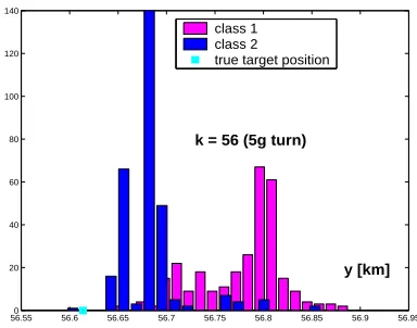
Figure 20 shows the clouds of the PF particles for both classes and the true target position indicated by a square. The particles corresponding to class 2 have higher likelihoods: conclusions can definitely be drawn that the target is of class 2. Figure
21 represents the MKFy-position histogram at time instant k = 56(at the
begin-ning of the5g turn). The particles corresponding to class 2 are in proximity to the
true target position. They quickly adapt to the changeable target dynamics.
Test trajectory 3. The trajectory is similar in shape to the previous scenario 2. The
target performs four turn maneuvers with normal accelerations−1g, 2g, −5g,4g,
displayed in Figure 22(b). In scenario 2, the target speed of 260 [m/s] provided
better conditions for the probability that the target belongs to class 2 according to
the speed constraints. Now the target speed is245 [m/s]and the speed information
is insufficient to distinguish the classes. The short-durable −5g turn is followed
by a 4g turn, which is located between the acceleration constraints, bounding the
classes - 2g and 5g. The situation is vague from the point of view of the
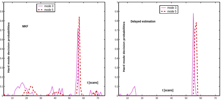
classifi-cation logic. It is difficult for the MKF to solve the classificlassifi-cation task - within 100 Monte Carlo runs, there are more than 50 realizations with wrong classification. The posterior mode probabilities can help to choose between : making the decision on the class now or postponing it to the future time. The delayed-pilot sampling algorithm provides more reliable mode information. It can be seen from Figures 23
by the models 3and5 of class two filter. The −5g turn is short-durable (2 scans) and the effect of the delayed estimation is comparably small. That is why the hard mode decision probabilities, obtained by the delayed-pilot MKF are a little better than the respective values of the MKF (see Figure 23(b) ). The next maneuver of a
4g turn is longer and lasts4scans. The acceleration of40 [m/s2]along the y-axis
is processed consecutively by models2and4of the filter for class two. The4gturn
is identified by the delayed-pilot MKF with a probability of 0.88 (Figure 24(b)),
while the probability of the conventional MKF is 0.35. The posterior probabilities of the last two maneuvers, provided by the delayed-pilot MKF give a consistent information for putting off the classification decision. The experiments with the
delayed estimation are realized with a time delay of two steps (△= 2).
The following inferences can be drawn from the experiments. The results obtained by the MKF approach for solving the JTC problem confirm the theoretical infer-ences [27], that the MKF can provide better estimation accuracy compared to the particle filter. The lower peak dynamic errors of the MKF are particularly useful for the classification task. This enables tracking and classifying objects of quite differ-ent types, with rather distinct dynamic parameters. This capability ensures some robustness of the algorithm, because the designed type parameters are not always precisely known.
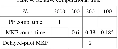
The MM PF and MKF computational complexity allow for an on-line imple-mentation. An advantage of the MKF is its reduced complexity compared to the
MM PF. The MKF was investigated in the cases of three sample sizes: Nc =
300,200, and 100. The relative computational time of the PF versus the MKF is
presented in Table 4. The computational time for a PF with Nc = 3000 particles
is considered as a reference time, which is compared to the MKF computational time. The experiments are performed on PC computer with AMD Athlon processor 2 GHz. Both algorithms permit parallelization at least of some parts : the MM fil-ters corresponding to each class can definitely be run in parallel. The delayed-pilot
MKF is realized with a sample sizeNc = 200and a delay of two steps (△= 2). It
[image:22.595.167.414.552.655.2]is 3 times more computational time consuming compared to the MKF.
Table 4. Relative computational time
Nc 3000 300 200 100
PF comp. time 1
MKF comp. time 0.6 0.38 0.185
0 10 20 30 40 50 60 70 0 10 20 30 40 50 60 70 80 90 100
x [km]
y [km]
START
RADAR
Fig. 2. Test trajectory 1
0 10 20 30 40 50 60 70 80
140 160 180 200 220 240 260 280 300 t [scans]
Position RMSE [m]
output estimate class 1 estimate class 2 estimate
Fig. 3. PF position RMSE [m] (traj. 1)
0 10 20 30 40 50 60 70 80
140 160 180 200 220 240 260 280 300 t [scans]
Position RMSE [m]
output estimate class 1 estimate class 2 estimate
Fig. 4. MKF position RMSE [m] (traj. 1)
0 10 20 30 40 50 60 70 80
20 40 60 80 100 120 140 160 180 200 t [scans]
Speed RMSE [m/s]
output estimate class 1 estimate class 2 estimate
Fig. 5. PF Speed RMSE [m/s] (traj. 1)
0 10 20 30 40 50 60 70 80
20 40 60 80 100 120 140 160 180 200 t [scans]
Speed RMSE [m/s]
output estimate class 1 estimate class 2 estimate
Fig. 6. MKF Speed RMSE [m/s] (traj. 1)
0 10 20 30 40 50 60 70 80
0 0.2 0.4 0.6 0.8 1 t [scans]
[image:23.595.90.490.71.636.2]class # 1 class # 2
0 10 20 30 40 50 60 70 80 0 0.2 0.4 0.6 0.8 1 t [scans]
[image:24.595.86.490.73.231.2]class # 1 class # 2
Fig. 8. PF class probabilities calculated us-ing both speed and acceleration constraints (traj. 1)
0 10 20 30 40 50 60 70 80
0 0.2 0.4 0.6 0.8 1 t [scans]
class # 1 class # 2
Fig. 9. PF normalized speed likelihoods (traj.1)
0 10 20 30 40 50 60 70 80
0 0.1 0.2 0.3 0.4 0.5 0.6 0.7 0.8
Posterior mode probabilities − class1 t [scans]
1
2
3
4
5
Fig. 10. MKF posterior mode probabilities - class 1 (traj. 1)
0 10 20 30 40 50 60
0 10 20 30 40 50 60
x [km]
y [km]
START
RADAR
Fig. 11. Test trajectory 2
0 10 20 30 40 50 60 70 80
100 200 300 400 500 600 700 t [scans]
Position RMSE [m]
output estimate class 1 estimate class 2 estimate
Fig. 12. PF position RMSE [m] (traj. 2)
0 10 20 30 40 50 60 70 80
120 140 160 180 200 220 240 260 280 300 t [scans]
Position RMSE [m]
output estimate class 1 estimate class 2 estimate
[image:24.595.89.491.81.433.2]0 10 20 30 40 50 60 70 80 20 40 60 80 100 120 140 160 180 200 t [scans]
Speed RMSE [m/s]
output estimate class 1 estimate class 2 estimate
Fig. 14. PF speed RMSE [m/s] (traj. 2)
0 10 20 30 40 50 60 70 80
20 40 60 80 100 120 140 160 180 200 220 t [scans]
Speed RMSE [m/s]
output estimate class 1 estimate class 2 estimate
Fig. 15. MKF speed RMSE [m/s] (traj. 2)
0 10 20 30 40 50 60 70 80
0 0.2 0.4 0.6 0.8 1 t [scans]
class # 1 class # 2
Fig. 16. Class probabilities (without speed constraints) (traj. 2)
0 10 20 30 40 50 60 70 80
0 0.2 0.4 0.6 0.8 1 t [scans]
[image:25.595.87.495.64.695.2]class # 1 class # 2
Fig. 17. Class probabilities (speed con-straints) (traj. 2)
0 10 20 30 40 50 60 70 80
0 0.2 0.4 0.6 0.8 1 t [scans]
class # 1 class # 2
Fig. 18. Normalized speed likelihoods (traj. 2)
0 10 20 30 40 50 60 70 80
0 0.1 0.2 0.3 0.4 0.5 0.6 0.7 0.8 0.9 1
Posterior probabilities − class2
1
2
3
4 5
[image:25.595.89.489.74.237.2]38 40
42 44
54 56 58 60 0 0.005 0.01 0.015 0.02 0.025
x [km] y [km]
weights
[image:26.595.188.386.92.242.2]class 1 class 2 true position
Fig. 20. PF - cloud of particles and associated weights at scan 57 - 5g turn (traj. 2)
56.550 56.6 56.65 56.7 56.75 56.8 56.85 56.9 56.95 20
40 60 80 100 120 140
y [km] k = 56 (5g turn)
[image:26.595.191.383.298.449.2]class 1 class 2 true target position
Fig. 21. MKF y-position histogram (traj. 2)
10 20 30 40 50 60 70
10 20 30 40 50 60 70
x [km]
y [km]
START
10 20 30 40 50 60 70
−60 −40 −20 0 20 40 60
t [scans]
normal acceleraions [m/s2]
[image:26.595.112.468.507.680.2]10 20 30 40 50 60 70 0
0.1 0.2 0.3 0.4 0.5 0.6 0.7 0.8 0.9 1
MKF
t [scans]
Hard mode decision probabilities
mode 3 mode 5
10 20 30 40 50 60 70
0 0.1 0.2 0.3 0.4 0.5 0.6 0.7 0.8 0.9 1
t [scans]
Hard mode decision probabilities
Delayed estimation
[image:27.595.112.467.73.236.2]mode 3 mode 5
Fig. 23. Hard decision for5gmaneuver (modes 3 and 5) for class 2
10 20 30 40 50 60 70
0 0.1 0.2 0.3 0.4 0.5 0.6 0.7 0.8 0.9
MKF
t [scans]
Hard mode decision probabilities
mode 2 mode 4
10 20 30 40 50 60 70
0 0.1 0.2 0.3 0.4 0.5 0.6 0.7 0.8 0.9
t [scans] Delayed estimation
Hard mode decision probabilities
[image:27.595.111.467.265.432.2]mode 2 mode 4
Fig. 24. Hard decision for4gmaneuver (modes 2 and 4) for class 2
5 Conclusions
type classification. A generalization of the algorithms’ application to the three-dimensional case is straightforward. In complicated target scenarios, the posterior mode probabilities can help in choosing from two possibilities: to make the de-cision on the class now or to postpone it to the future time. The posterior mode probabilities, provided by the delayed-pilot MKF offer a more reliable information for decision making.
Although the effectiveness of the developed PF and MKF algorithms is demon-strated over measurements from a single sensor their application over a network of sensors is possible and it is an open issue for future research.
Acknowledgements.The authors are thankful the reviewers which valuable comments helped for improving considerably the paper. This research is supported by the Bulgarian Foundation for Scientific Investigations under grants I-1202/02 and I-1205/02 and in part by the UK MOD Data and Information Fusion Defence Technology Center.
References
[1] S. Challa and G. Pulford, “Joint target tracking and classification using radar and ESM sensors,” IEEE Trans. on Aerosp. and Electr. Syst., vol. 37, no. 3, pp. 1039–1055, 2001.
[2] B. Ristic, N.Gordon, and A. Bessell, “On target classification using kinematic data,”
Information Fusion, vol. 5, pp. 15–21, 2004.
[3] A. Farina, P. Lombardo, and M. Marsella, “Joint tracking and identification algorithms for multisensor data,” IEE Proc.-Radar Sonar, Navig., vol. 149, no. 6, pp. 271–280, 2002.
[4] N. Gordon, S. Maskell, and T. Kirubarajan, “Efficient particle filters for joint tracking and classification,” in Proc. SPIE Signal and Data Processing of Small Targets, vol. 4728, Orlando, USA, April 1–5 2002.
[5] H. Leung and J. Wu, “Bayesian and Dempster-Shafer target identification for radar surveillance,” IEEE Trans. Aerosp. and Electr. Syst., vol. 36, no. 2, pp. 432–447, 2000.
[6] P. Smets and B. Ristic, “Kalman filter and joint tracking and classification in the TBM framework,” in Proc. of the Seventh Intl. Conf. on Information Fusion, Stockholm, Sweden, 2004, pp. 46–53.
[7] H. J. Zimmerman, Fuzzy Set theory – and its applications. Kluwer, Dordrecht, the
Netherlands, 1996.
[8] E. Blasch and C. Yang, “Ten methods to fuse GMTI and HRRR measurements for joint tracking and identification,” in Proc. of the 7th Intl. Conf. on Multisensor Information
Fusion, Stockholm, Sweden, 2004, pp. 1006–1013.
[10] B. Ristic, S. Arulampalam, and N. Gordon, Beyond the Kalman Filter: Particle Filters
for Tracking Applications. Artech House, Feb. 2004.
[11] S. Challa and N. Bergman, “Target tracking incorporating flight envelope information,” in Proc. of the Third Int. Conf. Inform. Fusion, Paris, France, July 2000.
[12] D. Salmond, D. Fisher, and N. Gordon, “Tracking and identification for closely spaced objects in clutter,” in Proc. of the Europ. Contr. Conf., Brussels, Belgium, 1997.
[13] M. Malick, S. Maskell, T. Kirubarajan, and N. Gordon, “Littoral tracking using particle filter,” in Proc. of the Fifth Int. Conf. Information Fusion, USA, July 2002.
[14] S. Herman and P. Moulin, “A particle filtering appropach to FM-band passive radar tracking and automatic target recognition,” in Proc. of the IEEE Aerospace Conf., Big Sky, Montana, March 2002.
[15] V. Jilkov, D. Angelova, and T. Semerdjiev, “Filtering of hybrid systems: Bootstrap versus IMM,” in Proc. of the European Conf. on Circuit Theory and Design, Budapest, Hungary, 1997, pp. 2: 873–858.
[16] S. McGinnity and G. Irwin, “Multiple model bootstrap filter for maneuvring target tracking,” IEEE Trans. on Aerospace Systems, vol. 36, no. 3, pp. 1006–1012, Dec. 2000.
[17] Y. Boers and J. Driessen, “Interacting multiple model particle filter,” IEE Proceedings
- Radar, Sonar and Navigation, vol. 149, no. 5, pp. 344–349, Oct. 2003.
[18] H. Driessen and Y. Boers, “An efficient particle filter for jump markov nonlinear systems,” in Proc. of the IEE Seminar Target Tracking: Algorithms and Applications, Sussez, UK, March 23-24 2004.
[19] D. Angelova, L. Mihaylova, and T. Semerdjiev, “Monte Carlo algorithm for maneuvering target tracking and classification,” in Lecture Notes in Computer Science.
ICCS Proc. Part IV, 4th Intl. Conf., M. Bubak and G. Dick van Albada and P. Sloot and
J. Dongarra, Ed. Krakow, Poland: Springer, 2004, vol. LNCS 3039, pp. 531–539.
[20] D. Angelova and L. Mihaylova, “Sequential Monte Carlo algorithms for joint target tracking and classification using kinematic radar information,” in Proc. of the Seventh
Intl. Conf. on Information Fusion, Stockholm, Sweden, 2004, pp. 709–716.
[21] X. Wang, R. Chen, and D. Guo, “Delayed-pilot sampling for mixture kalman filter with application in fading channels,” IEEE Trans. on Signal Processing, vol. 50, no. 2, pp. 241–254, Feb. 2003.
[22] A. Doucet, N. Gordon, and V. Krishnamurthy, “Particle filters for state estimation of jump Markov linear systems,” IEEE Trans. on Signal Proc., vol. 49, no. 3, pp. 613– 624, 2001.
[23] Y. Bar-Shalom and X.-R. Li, Estimation and Tracking: Principles, Techniques, and
Software. Norwood, MA: Artech House, 1993.
[25] A. Tchamova, T. Semerdjiev, and J. Dezert, “Estimation of target behaviour tendencies using Dezert-Smarandache theory,” in Proc. of the Sixth Intl. Conf. Inform. Fusion, Australia, July 2003, pp. 1349–1356.
[26] J. S. Liu and R. Chen, “Sequential Monte Carlo methods for dynamic systems,”
Journal of the American Statistical Association, vol. 93, no. 443, pp. 1032–1044,
1998. [Online]. Available: citeseer.nj.nec.com/article/liu98sequential.html
[27] R. Chen and J. S. Liu, “Mixture Kalman filters,” Journal of the Royal Statistical
Society B, no. 62, pp. 493–508, 2000.
[28] Z. Chen, “Bayesian filtering: From Kalman filters to particle filters, and beyond,” Adaptive Syst. Lab., McMaster Univ., Hamilton, ON, Canada. [Online],
http://soma.crl.mcmaster.ca/˜zhechen/homepage.htm, 2003.
[29] R. Chen, X. Wang, and J. Liu, “Adaptive joint detection and decoding in flat-fading channels via mixture Kalman filtering,” IEEE Trans. on Inform. Theory, vol. 46, no. 6, pp. 493–508, 2000.
[30] G. Casella, “Statistical inference and Monte Carlo algorithms,” Test, vol. 5, pp. 249– 344, 1997.
[31] X. R. Li and V. Jilkov, “A survey of maneuveuvering target tracking. Part I: Dynamic models,” IEEE Trans. on Aerospace and Electr. Systems, vol. 39, no. 4, pp. 1333–1364, 2003.
[32] Y. Bar-Shalom and X.-R. Li, Multitarget-Multisensor Tracking: Principles and