Version: Published Version
Monograph:
Miraldo, M. (2007) Reference pricing versus co-payment in the pharmaceutical industry: :
price, quality and market coverage. Working Paper. CHE Research Paper . Centre for
Health Economics, University of York , York, UK.
[email protected] Reuse
Items deposited in White Rose Research Online are protected by copyright, with all rights reserved unless indicated otherwise. They may be downloaded and/or printed for private study, or other acts as permitted by national copyright laws. The publisher or other rights holders may allow further reproduction and re-use of the full text version. This is indicated by the licence information on the White Rose Research Online record for the item.
Takedown
If you consider content in White Rose Research Online to be in breach of UK law, please notify us by
Reference Pricing Versus Co-Payment
in the Pharmaceutical Industry:
Price, Quality and Market Coverage
Reference Pricing Versus Co-Payment in the
Pharmaceutical Industry:
Price, Quality and Market Coverage
Marisa Miraldo
Centre for Health Economics
University of York
York YO10 5DD
Email: [email protected]
The new CHE Research Paper series takes over that function and provides access to current research output via web-based publication, although hard copy will continue to be available (but subject to charge).
Acknowledgements
This article has been strongly improved with comments by Hugh Gravelle, Matteo Galizzi, Michael Kuhn, Pau Olivela, Peter C. Smith, Xavier Martinez Giralt and participants of the iHEA World Congress (held in 2005 in Barcelona) to whom I am grateful. This paper was written with financial support from the Sub-Programa Ciência e Tecnologia do 2o Quadro Comunitário de Apoiodo
Ministério da Ciência e Tecnologia and Fundação Calouste Gulbenkian, both in Portugal.
Disclaimer
Papers published in the CHE Research Paper (RP) series are intended as a contribution to current research. Work and ideas reported in RPs may not always represent the final position and as such may sometimes need to be treated as work in progress. The material and views expressed in RPs are solely those of the authors and should not be interpreted as representing the collective views of CHE research staff or their research funders.
Further copies
Copies of this paper are freely available to download from the CHE website http://www.york.ac.uk/inst/che/publications. Access to downloaded material is provided on the understanding that it is intended for personal use. Copies of downloaded papers may be distributed to third-parties subject to the proviso that the CHE publication source is properly acknowledged and that such distribution is not subject to any payment.
Printed copies are available on request at a charge of £5.00 per copy. Please contact the CHE Publications Office, email [email protected], telephone 01904 321458 for further details.
Centre for Health Economics Alcuin College
University of York York, UK
www.york.ac.uk/inst/che
copayment reimbursement on firms pricing and quality strategies as well as on market coverage under different market structures: competitive market, local monopolies and exogenous full market coverage. Results allow us to shed some light on the welfare and total drug expenditure implications of different drug reimbursement policies.
1
Introduction
In this paper we aim at comparing two of the most common drug Þnancing mechanisms: reference pricing and co-payment trying to clarify the broadly ac-claimed positive aspects of reference pricing against co-payment systems. Refer-ence Pricing (RP) is a regulatory mechanism aimed at controlling pharmaceuti-cal expenditure in terms of their impact on quality, market coverage and prices. The mechanism consists of clustering drugs according to some equivalence cri-teria (chemical, pharmacological or therapeutic) and deÞning a reference price for each cluster. The third party payer, then, will just reimburse not more than that price for each drug on that cluster. If a consumer buys a drug with price lower or equal to the reference price of that cluster, then the co-payment he faces is null. Otherwise, if the drug bought is priced higher than the reference price, the consumer will pay the difference between the reference price and the drug price.
Even though its formulation varies from country to country, RP is gener-ally seen as an efficient mechanism in cutting drug prices by encouraging self restraint, in controlling relative demand of highly priced drugs and in encour-aging the appropriate use of drugs. Based on this premise, third party payer’s pharmaceutical expenditure would be controlled. However, the effectiveness of this mechanism strongly depends on its ability in enhancing competition in the drug market and on the promotion ofÞnancial responsibility by consumers and pharmaceuticalÞrms.
In our opinion, there are two crucial points concerning RP regulation: its efficacy in achieving the goals it aims for, and its discriminatory effects. Con-cerning the Þrst, it is important to identify the cause of high pharmaceutical expenditure. Indeed, drug expenditure is driven by two factors: high prices and high consumption Lopez-Casasnovas and Puig-Junoy [5] state that RP as a procurement mechanism would indeed be effective if the market fulÞls a speciÞc structure, namely, a large buyer, wide product coverage and low demand elastic-ity. If RP ends up reducing prices, it might not end up reducing pharmaceutical expenditure if drug consumption is very high.
Furthermore, by clustering drugs that might not be perfect substitutes one can expect that due to patient characteristics RP might lead to undesirable effects such as discrimination against Þrms and patients1. If patients select
one of the drugs priced below the RP just to avoid the co-payment, we might expect a lower level of treatment effectiveness and even an increase in expenses if, afterwards, the patient needs complementary treatment2.
1Zammit-Lucia and Dasgupta [9] cite the case of a patient suffering different averse affects
when using different drugs in the same cluster. The patient suffered severe averse effects from one calcium antagonism with one drug but tolerated the other drug classiÞed in the same cluster.
2This situation is aggravated if one considers that patients are not perfectly informed about
Weak substitutability between drugs in the same cluster is quite likely to occur due to a wide range of drugs’ characteristics: differences in drug qual-ity, performance, differences in chemical preparation, in application form, bio-availability, number and type of indications, side effects, to name some [6]. These drug speciÞcations can be of higher or lower relevance depending on the speciÞc patient to whom the drug will be administrated. If, from a speciÞc pa-tient point of view, there is no interchange-ability then the co-payment becomes non avoidable and, consequently, RP discriminates against the patient whenever opting for a drug whose price is higher than the RP level. Therefore, unjustiÞed inequalities between patients might then arise if RP fails to take into account patient heterogeneity.
The literature on RP is scarce and not all the subjects addressed above have been covered. It urges the development of theoretical set ups in order to better understand incentives of this policy and, even more importantly, to develop optimal Reference Pricing policies.
The studies by Mestre Ferrandiz and Merino-Castelló deserve special atten-tion ([8], [7]). The generic paradox arises on the work by Mestre-Ferrandiz [8]. The author compares the impact of a reference price and a co-payment system in a pharmaceutical market with generic competition. Using a horizontal dif-ferentiated model where twoÞrms competeá la Bertrand, the author concludes that, just for some RP level, a RP policy can control pharmaceutical expendi-ture and reduce drug prices. Even though some welfare analysis is developed, the author doesn’t explicitly solve for optimal reference pricing.
Merino-Castello [7], studies the impact of RP on the price setting strategies of pharmaceuticalÞrms (generic and branded) on a vertical product diff erenti-ated model. The author concludes that RP is indeed effective in enhancing price competition as, after RP had been implemented, branded prices decrease while generic prices remain constant. Nevertheless, this price competition increases the usage of branded drugs in detriment of generics.
We believe, however, that, when patients are heterogeneous, the effect of RP on price competition would be lower because of a market segmentation effect. In fact, if there exists consumer heterogeneity in terms of price elasticity, drugs that are not perfectly substitutable will beneÞt from some market power even after RP has been introduced, and henceÞrms will keep on pricing above the reference price level. If this is the case, a subset of consumers would not be able to avoid the co-payment, thus being indeed discriminated by RP. On the contrary, it might also be the case that due to lack of information part of the demand ends not buying the drug that better matches his speciÞcations, switching to a less-than optimal cheaper drug in order to avoid the co-payment. If this is the case, RP might lead to patients being prescribed drugs not perfectly suitable for their health condition, leading to a lower health outcome, or, if patients need complementary treatment, or drugs, even to increases in health care costs. Clearly, to fully take into account patients’ heterogeneity, it would be necessary
to consider both horizontal and vertical differentiation. In fact, our analysis differs from the two above mentioned contributions in several aspects.
Firstly, in order to capture the effects of both quality and consumers’
speci-Þcities on the decision of buying a drug, we complement a model of vertical differentiation with an horizontal dimension3 and for consumer heterogeneity
along the horizontal dimension. Thus, while letting each patient have their best-preferred drug, we assume that patients are homogeneous in what con-cerns their preferences for quality4: everything else equal, all the consumers
prefer higher to lower quality drugs. As the inclusion of a two dimensional differentiation might be a controversial subject in the pharmaceutical market modelling, a deeper justiÞcation may be useful before proceeding.
We intend asquality of a pharmaceutical product, all the characteristics af-fecting its efficacy. Differences in quality might arise from differences in coating, in the production process (for instance, rates of agitation and pH during the production process), in the degrees of purity of the active compound, just to name some. These differences may affect the efficacy of a drug, for instance, by affecting the rate of absorption of the active compound. Despite this homo-geneity, consumers differ on their most preferred drug, because of consumers’ individual speciÞcities. This assumption can be exempliÞed in several ways. For example, when faced with the choice of two drugs, clustered in the same group, consumers might be constrained to buy one speciÞc drug due to adverse side effects that arise when combining the second drug with the already active medication, or even because of the side effects of the drug when administrated alone.
Another example is patient intolerance or "neutrality" to a speciÞc active compound. In fact, differences in metabolism, existence of concurrent diseases, gastric pH, bacterialßora, among others, inßuence the tolerability and efficacy of a speciÞc drug.
To provide a general example, two drugs are said to be horizontal diff erenti-ated when, for a speciÞc patient, one has side adverse affects and the other not. On the other hand, the same drugs are said to be vertically differentiated if, for all patients, their efficacy is different due to different rates of absorption caused by drugs’ characteristics (e.g. different coatings). Therefore, two consumers that differ on their most preferred drug, when deciding between two drugs with the same active compound (i.e. zero horizontal differentiation), will base their choice on the drugs’ levels of quality. This case is well illustrated when we con-front generic and branded drugs. As we have claimed before, these drugs might not have the same quality, or, maybe better, consumers might perceive their qualities as different. On the other hand, if the same consumers have to choose between drugs with different active compounds, their choice will depend on 3Note that we do not solve for drugs locations, we simply assume that drugs are horizontally
differentiated but that the location of eachÞrm having been chosen in a previous stage not contemplated in our model.
4One can think of it as quality (vertical differentiation) or perceived quality (virtual
the trade offbetween higher (lower) quality and lower (higher) substitutability between the drugs.
In the former case, we might expect RP policies to have a discriminatory effect againstÞrms if quality differences are not accounted for: by reimbursing the same amount for all the qualities, the government is in fact favouring low quality Þrms and providing incentives to lower the level of quality produced. In the latter case, the discriminatory effects are also against consumers if RP fails to account for patients’ heterogeneity5. Consequently, it is important to
distinguish between the two differentiation dimensions. Even though both have implications on consumers’ utility, the source of those effects differs: as concerns vertical differentiation, the implications for patients’ utility are exclusively due to the drug characteristics, while, concerning horizontal differentiation, those effects depend on the consumer speciÞcities. We argue that this is a crucial point to be taken into account in the design of drugs’ reimbursement policies.
Moreover, and contrary to the existing literature, we assume patients to have the sameÞnite willingness to pay for quality.
Finally, we also make some considerations on optimal reference pricing poli-cies. Brekke, Nuscheler and Straume [2] have developed a set up that includes some of these features. They study, in a model of spatial competition, the effect of a price regulation mechanism, where the regulator sets the prices, on the qual-ity and location variables. However, in their model patients are homogeneous on their tastes and RP is not analysed.
There are several questions that are worthwhile analysing: If patients do indeed have different degrees of substitutability between two drugs, is it optimal to settle a unique reference price level for those two drugs, independently of patients’ degree of substitutability between those same drugs? What are the effects of such a policy on the quality of the drugs in the market? How does this affect welfare? Is it efficient in the control of health expenditure? If yes, who is paying the cost reduction? To answer these questions, we analyse the effect of RP on equilibrium outcomes, having as a benchmark a co-payment system, in a model where drugs are horizontally differentiated and whereÞrms also decide on optimal quality. Firms choose prices and quality, and patients are assumed to be heterogeneous, in that each patient has its best-preferred drug. Within this framework we analyse the impact of co-payment reimbursement and reference pricing on drugs prices, quality and market coverage under different market structures, namely, competitive market, local monopolies and exogenous market coverage, highlighting welfare and cost control implications.
5Assuming that patients stil buy their most preferred drug even when its price is higher
2
The model
2.1
A speci
Þ
c model for pharmaceuticals
While the main qualitative results by Economides (1984) [3] clearly still apply to our model, however, in order to betterÞt the very nature of pharmaceuti-cals markets, we introduce three important innovations which require particular attention.
First, in our model varieties are treated, unlike Economides [3], as exoge-nously given. Therefore, our model is clearly unable to provide an equilibrium location choice comparable with Economides result against the acclaimed "Prin-ciple of Minimum Differentiation".
Secondly, and crucially, we introduce a second, vertical, dimension in the analysis. In fact, Þrms endogenously choose the quality levels at which they provide the differentiated drug. This, in turn, directly affects consumers util-ity, by the new elementqirp, and therefore substantially drives patients’ choice whether, and, if so, what to buy.
Finally, and most importantly, our main objective is to investigate the above quality-then-price duopoly game in presence of areimbursement policy. In fact, in most of the pharmaceutical markets in Europe patients are partially subsi-dized bythird party payers, such as the national health service or the insurance companies, according to some speciÞc reimbursement rule.
In particular, two principal health careÞnancing schemes have been largely adopted with regards to private expenditure on drugs. On the one hand, the traditionalco-payment system reimburses the patients a proportional fraction of all drugs’ prices. On the other hand, the more recentreference pricing system refunds patients a lump sum amount independently of the price of the drugs actually bought.
We argue, however, that different reimbursement policies may have an im-pact on patients’ demand, thus affectingÞrms’ strategies and equilibrium quali-ties and prices. To better illustrate the role of co-payment and reference pricing in thequality-then-price duopoly game are considered in the next sections.
2.2
Firms and products
There aretwoÞrms, each producing a drug at an identical marginal costc, for simplicity normalized to zero. Firm 1 produces drug 1 and Firm 2 produces drug 2. Drugs are horizontally differentiated à la Hotelling [4], being located in an unidimensional characteristics space as represented by the unit interval
[0,1]. In particular, we assume that varieties{x1, x2}∈[0,1]have already been
chosen, byÞrm 1 and 2 respectively, as outcomes of a previous decision process, and that they are therefore treated as exogenously given in our model.6
Varieties can be thought as associated each to a speciÞc composite need for a speciÞc health treatment. Equivalently, the unit interval[0,1]can be interpreted 6Locations are assumed to be exogenous since a model with endogenous locations as well
as a cluster containing all the different, but related, drug varieties designed for a close family of comparable health dysfunctions: for instance, any drug treating
ßue, or gastritis, or throat cancer and so on. On the other hand, drugs are also vertically differentiated in that, for each variety, a continuum of possible quality speciÞcations is possible. Given a speciÞc variety, higher quality drugs are most effective in treating the relative health disease, and are then preferred by any patient having that speciÞc horizontal characteristic. Furthermore, each Þrm select aquality-price strategy in order to maximize its proÞt function, within a two-stages non-cooperative game.
2.3
Timing
In fact, we assume thetiming of the model being as follows. Before the game starts, a given pair of drug varietiesx1, x2∈[0,1]has been exogenously selected
byÞrms. By a standard convention,x1≤x2.
In the Þrst stage, given drug varieties, each Þrm i= 1,2chooses, indepen-dently and simultaneously, the quality speciÞcationqirp of its own drugxi.
In the second stage, being both varieties and qualities common knowledge, eachÞrmi= 1,2, again simultaneously and independently, chooses its pricepi. After the two stages of strategic decisions by the Þrms, all the consumers just choose which preferred drug variety to buy, if any, and all the payoffs are consequently worked out.
We believe such a timing canÞt quite well the genuine essence of competition in drugs markets.
In fact, most of the times, the decision to undertake the production of a spe-ciÞc drug variety implieslong-runinvestments, both inR&D and in technology, which are planned and implemented long in advance to the consideration of a possible market structure. Indeed, long-run scientiÞc progress, technological advancements, research outcomes and patents are much more likely to represent explanatory factors for the entry into a drugs line, than strategic considerations in terms of actions and reactions by potential competitors.
On the other hand, given the long-run decision of locating at a speciÞc drug variety, medium-run adjustments in the relative qualitative level are certainly possible. Moreover, such a decision can hardly be thought as being independent from the consideration of the strategies by competitors already active in the production of the same drug, or of close varieties.
Finally, in theshort-run, given the varieties and the quality levels produced in the market, each Þrm can compete by setting its price at an optimal level, given the competitors’ pricing behaviour.
2.4
Strategies
Theactions by eachÞrm i= 1,2consist of the choice of a quality levelqrpi ∈ Qi =
£
of the art, andQ=Q1×Q2.7
A strategy forÞrmi = 1,2is then represented by aquality-price pairσi ∈ Σi =Qi×PiQ, wherePiQ:Q−→Pi is a correspondence from the space of the chosen quality levels to some price.
Finally, no explicit strategic behaviour is described for consumers, who just choose whether to buy or not, and if so, which drug to buy, taking as given varieties, qualities and prices set byÞrms.
2.5
Equilibrium Solution
The model being a game of perfect information with sequential stages of simul-taneous moves, the relevant solution concept for the game is clearly theSubgame Perfect Nash Equilibrium.
In particular, Þniteness in the number of stages allows us to proceed by backward induction. First, we will look for the equilibrium price conÞgurations associated to generic pairs of qualities(q1, q2)in the price subgame, then, we will
solve for the mutually optimal qualities in theÞrst stage, and we will describe theequilibrium quality andprice strategies of the overall game.
For simplicity, in the analysis we will only focus onpure strategies Subgame Perfect Nash Equilibrium.
2.6
Consumers Utility Function and Demand
Consumers are heterogeneous in their tastes for drugs. Each consumer is as-sumed to have a most preferred drugzthat is given by his location on the[0,1]
line segment. In particular, we assume a mass of consumers standardized to1
anduniformly distributed along the unit interval.
Importantly, consumers are endowed with a Þnite instant utility k when consuming one of the drugs, equal across all individuals. Each consumer is assumed to be restricted to buy just one unit from one single drug variety, or none and, in aÞrst instance, we further assume that there are always possible non buyers in the market.
In fact, given drugs’ varieties, qualities and prices, patients decide whether to buy one unit of drugx1, one unit of drugx2, or,Þnally, not to buy any drug
at all.
In absence of any reimbursement policy, the model closely resembles the one by Economides [3] . In fact, denote, fori= 1,2, xi the drug ivariety, qrpi the drugiquality,pi the drugiprice, andtthedisutility transportation cost.
As in Economides (1984), we assume that the consumers’ preferences para-meter k is Þnite, and that the disutility incurred by a consumer located at z
consuming drugxi is linear in the distance between the horizontal characteris-tics,t|z−xi|.8
7This assumption will, further in the chapter, allow us to deÞne an equilbrium for the local
monopolies case.
8Note that linear transportation costs might lead to the non-existence of a price equilibrium
in pure strategies whenÞrms locations are close. Locations must be at most at 1
Therefore, in our model with no reimbursement policy, consumer z utility by consuming drugi, fori= 1,2is given by
U(z;xi) =k+qirp−pi−t|z−xi|
If the consumer does not buy any of the drugs his utility is assumed to be
U(z; 0) = 0.
As shown by Economides (1984), the level of k is in fact crucial in the determination of demand and of the consequent market structure. Indeed, for high enough instant utility from treatment, consumers always buy some of the differentiated products and consequently the market is fully covered. This case indeed encompasses the equivalent analysis by D’Aspremont, Gabszewicz and Thisse [1] with an inÞnite instant utility from treatment. However, for medium levels of the instant utility from treatment parameter, consumers at the edges of the market choose to not consume any of the differentiated commodities, so that the market is only partially covered. Finally, for sufficiently low instant utilities from treatment, also consumers whose horizontal dimension preferences are close to the centre of the market, might be better offby not buying any of the differentiated products. In this caseÞrms behave as local monopolists, selling only to their relative neighborhoods.
3
Co-payment Reimbursement
We Þrst investigate the case where the expenses in pharmaceuticals are re-imbursed through a co-payment system: patients are rere-imbursed a fraction
0≤α≤1of drug prices.
3.1
Demand
By assuming, without loss of generality, unitary transportation costt= 1, the utility derived by a consumer located atzfrom buying drugiis given by
U =k+qrpi −(1−α)pi−|z−xi| i= 1,2 (1)
As mentioned above, the Þnite instant utility from treatment for patients (k) plays a crucial role in the determination of the market coverage.
The level of market coverage, in turn, has an important impact on the degree of competition betweenÞrms. Also in presence of a co-payment reimbursement, in fact, depending on market coverage, competition might be tighter or softer.
In particular, market conÞguration might be such thatduopoly competition occurs: the twoÞrms actively compete for serving the demand located in the centre of the market. Within this competitive scenario, it may also happen that all the consumers buy some drugs. In fact, the market is fully covered whenever patients show sufficiently high willingness to pay. However, for an intermediate instant utility from treatment k, consumers at the edges of the
market choose to not consume any of the differentiated commodities. In fact, even in a competitive scenario, the market can also be onlypartially covered. In such a case, reimbursement policy may be seen as not fully effective. Finally, it might also occur that the twoÞrms behave asnatural monopolies. In fact, for low willingness to pay, also patients located around the centre of the market may opt out of not buying anything. In this caseÞrms behave as local monopolists, selling only to their relative neighborhoods.
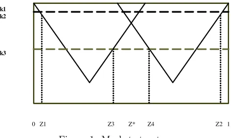
The market in the three cases can be represented in the following diagram,
0 Z1 Z3 Z* Z4 Z2 1
k1 k2
k3
0 Z1 Z3 Z* Z4 Z2 1
k1 k2
[image:16.595.185.421.238.379.2]k3
Figure 1: Market structures
Therefore, it can be noticed that demand has a kinked structure and, con-sequently, is not continuously differentiable everywhere. As this implies that proÞt functions are also not continuously differentiable everywhere, computing
Þrms’ best response functions may be not straightforward. To deal with this, in our model of co-payment scheme, we need to deÞne, for each demand segment, the respective proÞt function. These demand segments depend both on Þrms strategies and on the level of consumers’ treatment instant utilities.
3.1.1 Intermediate treatment instant utilities: the competitive sce-nario with partial coverage
Forintermediatevalues ofk, there are consumers at the edges of the market that do not buy any of the drugs. From now on we will refer to this case, illustrated in Figure 1 (fork2), as thecompetitive scenario with partial coverage. Denote
z as the location of the consumer who is indifferent between buying the drug produced byÞrm 1 and the drug produced by Þrm 2. Moreover, denote as z1
the location of the consumer indifferent between buying drug 1 or not buying any of the differentiated drugs existing in the market and as z4 the location
of the consumer indifferent between buying drug 2 or not buying any of the differentiated drugs existing in the market. As patients derive disutility from the distance between their most preferred drug and the drug they buy, we have that forz∈[0, z1[ we haveU(z;x2)< U(z;x1)< U(z; 0). On the other hand,
the intervalz ∈]z1, z[prefer buying Þrm’s 1 drug than buying drug 2 or than
not buying any drug at all. For z ∈ ]z, z4[ we have that U(z;x1) < U(z; 0)
< U(z;x2).Finally, also all the consumers located in the segmentz∈]z4,1], are
better offby not buying any drug at all: U(z;x1)< U(z;x2)< U(z; 0). Thus,
z1, z4 and z will be the solutions ofU(z; 0) =U(z;x1), U(z;x2) =U(z; 0)and
U(z;x2) =U(z;x1) respectively. Therefore, from the expression for the utility
function, we may immediately work out z1, z4 and z as functions of prices,
varieties and qualities:9
z1(p1, q1) = (1−α)p1+x1−k−q1 (2)
z(p1, q1;p2, q2) =
(1−α) (p2−p1) + (x1+x2) +q1−q2 2
z4(p2, q2) = k+q2+x2−(1−α)p2
As each consumer demands just one unit of drug and is assumed to be endowed with sufficient income to afford its price, total demand is given by
D=
z4
Z
z1
f(z)dzwithD1=
z
Z
z1
f(z)dzbeing served byÞrm 1 and the remaining
D2 =
z4
Z
z
f(z)dz consumers by Þrm 2. Thus, with z uniformly distributed on the support[0,1],Þrms demands are given by,
D1 = z−z1 (3)
D2 = z4−z
It can be seen that Þrms’ demands depend positively on the consumers’ instant utility from treatment k. Moreover, each Þrm’s demand increases in the competitor price and decreases in its own price. The impact ofαonÞrms’ demand depend on the pricing strategies
∂Di
∂pi
< 0, ∂Di ∂pj
>0
∂Di
∂α =
1
2(pi−pj) +pi i, j= 1,2i6=j
The effect of the reimbursement rate αin demand can be decomposed into two effects. Indeed, α affects both the consumers choosing to always buying from one of theÞrms and the consumers deciding whether to buy one unit of the differentiated product, or no product at all. Then, an increase inαincreases the number of the second type consumers and, depending onÞrms’ prices difference,
might increase or decrease the number of consumers that switch from one drug to the other.
If Þrms set equal prices, the impact of α on demand boils down to ∂Di
∂α =
pi: therefore, the reimbursement rate α has no impact on the allocation of consumers betweenÞrms, and only affects, positively, the number of consumers facing the decision of whether to buy something or not to buy at all. If a
Þrm sets a higher price, sayp2> p1 then an increase inαallows not only the
consumers currently not purchasing anything to buy fromÞrm 1, but also the ones currently buying fromÞrm 2 to switch toÞrm 1 instead.
3.1.2 High instant utility from treatment: the competitive scenario with full coverage
Forksufficientlyhighall consumers buy one of the drugs. In such a case, illus-trated inÞgure 1 (fork1), for anyz∈[0,1],U(z;xi)> U(z; 0): all consumers are better offby buying one of the drugs. We refer to this case as the competi-tive scenariowithfull coverage. The market is fully covered andÞrms’ demand functions are given by,
D1=z, D2= 1−z
Notice that, here, demand does not depend on the instant utility from treatment
k. Indeed, in this case, the instant utility from treatment k is assumed to be so big that the market is fully covered, and all consumers buy the differentiated product.
The effect of the reimbursement rate α on one Þrm’s demand depends on the its own price and the price of its competitor,
∂Di
∂α =
pi−pj
2 i, j= 1,2,i6=j
While in the previous case the reimbursement rate had an impact on both the choice of whether to buy or not and on the decision from which Þrm to buy, in this case the reimbursement rate only affects the allocation of consumers between drugs.
Concerning the effect of pricing strategies onÞrms’ demands we have that
∂Di
∂pi
<0, ∂Di ∂pj
>0 i, j= 1,2,i6=j
Again,Þrm’s demand is a decreasing function of its own price and increases in the competitor price.
3.1.3 Low instant utility from treatment k: local monopolies
Finally, for sufficientlylowtreatment instant utilities, consumers located close to the centre are better off by not participating in the market and, consequently,
U(z; 0). By referring to Figure 1 (fork3), letz1(p1)andz3(p1)be the consumers
indifferent between buying fromÞrm 1 whilez2(p2)andz4(p2)be the consumers
indifferent between buying fromÞrm 2 or not buying any of the drugs: in such a case we have that forz ∈{z1, z3}, U(z;x1) =U(z; 0) and forz ∈{z2, z4},
U(z;x2) =U(z; 0). Therefore, from the expression for the utility function, we
may immediately work outz1, z2, z3 andz4 as functions of prices, varieties and
qualities:
EachÞrm demand is then given by,
D1 = z3(p1, q1)−z1(p1, q1) (4)
D2 = z4(p2, q2)−z2(p2, q2)
Therefore, it can be seen thatÞrms demands are increasing in both the instant utility from treatment k and the reimbursement rateα. Moreover, the mag-nitude of the effect of αon one Þrm’s demand depends only on its own pricing strategy: ∂Di
∂α = 2pifor i = 1,2. Under local monopolies, the reimbursement rate has no effect on the distribution of consumers betweenÞrms. Indeed, under this market structure,Þrms do not compete for consumers, acting instead as a monopolist for a demand segment.
Demand does not depend on the competitors’ price and decreases in Þrm’s own price,
∂Di
∂pi
<0, ∂Di ∂pj
= 0 i, j= 1,2,i6=j
Naturally, the above described demand structure will imply a step proÞt function for bothÞrms, that we will describe in depth later.
3.1.4 Market coverage
Finally, letM (0≤M ≤1) be the number of consumers buying the diff erenti-ated product, i.e., the market coverage. GenerallyM is given by
M= min{z4,1}−max{z2, z}+ min{z3, z}−max{z1,0} (5)
Hence, when the market is served by two local monopolistsM=z4−z2+z3−z1.
In a competitive market with partial coverageM =z4−z1. Finally under full
coverageM= 1.10
Depending on the exogenous parametersk, x1 andx2the market conÞ
gura-tion will differ. Indeed we can have a competitive scenario, local monopolies or 1 0Furthermore, for sake of completeness, we should mention that, besides the three scenarios
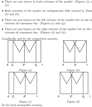
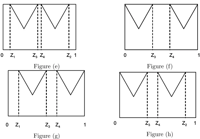
exogenous full market coverage. In a competitive scenario and in local monop-olies there are several possible sub conÞgurations namely:
• There are non buyers in both extremes of the market (Figures (a) and (e))
• Both extremes of the market are endogenously fully covered in (Figures (b) and (f))
• There are non buyers on the left extreme of the market but on the right extreme all consumers buy (Figures (c) and (g))
• There are non buyers on the right extreme of the market but on the left extreme all consumers buy (Figures (d) and (h))
Graphically and for the competitive scenario,
0 Z1 Z* Z2 1 0 Z1 Z* Z2 1
Figure (a)
0 Z* 1 0 Z* 1
Figure (b)
0 Z1 Z* 1 0 Z1 Z* 1
Figure (c)
0 Z* Z2 1 0 Z* Z2 1
[image:20.595.142.465.160.533.2]0 Z1 Z3 Z4 Z2 1
0 Z1 Z3 Z4 Z2 1
Figure (e)
0 Z3 Z4 1
0 Z3 Z4 1
Figure (f)
0 Z1 Z3 Z4 1 0 Z1 Z3 Z4 1
Figure (g)
0 Z3 Z4 Z2 1
0 Z3 Z4 Z2 1
Figure (h) In the following sections, then, we will analyse in greater details the duopoly two-stages game for the three above scenarios: competitive with full or partial coverage, and local monopolies. However in the main text we focus only on the cases illustrated in Þgures (a), (b), (e) and (f). The remaining cases can be found in appendix.
3.2
The price game
In this stageÞrms compete simultaneously in prices. Withpi the drug price of
Þrmi, andDithe demand faced byÞrmi, the duopolists proÞt functionsπiare given by,
πi =piDi−
q2
i
2 i= 1,2 (6)
As mentioned before, as the demand function is kinked, Þrms’ proÞt func-tions are segmented. Thus, given (4), if
0≤p1≤p2+
q1−q2 (1−α)+
x1−x2
(1−α) (7)
theÞrm will be a monopolist and the proÞt function is given by,
π1=p1(z4−z1)−q 2 1 2
Otherwise, if
p2+
q1−q2 (1−α)+
x1−x2
(1−α) ≤p1≤
q1+q2+x1−x2−(1−α)p2+ 2k
[image:21.595.165.498.118.349.2] [image:21.595.129.481.475.710.2]the market structure will be competitive and theÞrm 1 proÞt is given by,
π1=p1(z−z1)−
q2 1 2
Finally, if
if q1+q2+x1−x2−(1−α)p2+ 2k
1−α ≤p1≤
k+q1+x1
1−α (9)
the market structure will be characterized by local monopolies andÞrm 1 proÞt function is given by,
π1=p1(z3−z1)−
q2 1 2
We will now look for the Nash Equilibria in pure strategies (NE) of the simultaneous moves price game played by the twoÞrms in the last stage of the overall game.
A pricepi such that0≤pi ≤pj+q
rp i −qj
(1−α) +
xi−xj
(1−α) i, j= 1,2and i6=j, can
never constitute a pure strategies Nash Equilibrium of the price subgame. The proof consists of a standard undercutting argument. Within this price range one of theÞrms will be a monopolists and the secondÞrm would be out of the market, earning zero proÞts. The latter will always have incentives to undercut on the monopolist price strategy in order to gain the whole demand.
Having ruled out the monopolist case as a candidate Nash equilibrium in the price subgame, we will then focus on the two polar cases: competitive sce-nario, either with partial or full coverage, and the local monopolists scenario. Maximizing proÞts with respect to prices and solving theÞrst order conditions, the Nash Equilibrium in the price game for these two cases is summarized in the propositions that follow,
Proposition 1 Fork < x2−x1−q1+2q211with i, j= 1,2andi6=j the market
is characterized by two local monopolists and the Nash Equilibrium in the price stage is given by12,
p∗ilm= k+q
rp i
2 (1−α) i= 1,2 (10)
For q1−q2 > 117 (x2−x1) and k > 65x2− 32x1+ 31 −q2+2q113 the market is
1 1This inequality ensures that pi ∈ qi+qj+xi−xj−(1−α)pj+2k
1−α , k+qi
1−α and can be easily computed by plugging the equilibrium prices and solving fork.
1 2Second order conditions are always satisÞed. Indeed, ∂2
πi
∂p2
i
=−4 + 4α <0.
1 3These are market structure conditions. For reservation prices that satisfy these conditions
the market will be competitive. They are easily obtained by plugging the equilibrium prices in the conditionpi∈ pj+qi−qj
(1−α)+
x1−x2 (1−α),
qi+qj+x1−x2−(1−α)pj+2k
competitive and the Nash Equilibrium in the price stage is14
pc1∗ = 7 (x1−x2) + 3q2−17q1−14k 35 (α−1)
pc∗
2 =
7 (x1−x2) + 3q1−17q2−14k
35 (α−1) (11)
Forpi∈
hqrp
i +qj+x1−x2−(1−α)pj+2k
1−α ,
k+qirp
1−α
i
withi, j= 1,2andi6=j15 Þrms
do not compete for the marginal consumer. There are consumers in the centre of the market that are better offby not buying any of the drugs. Hence,Þrms behave like local monopolists.
Notice, however, that if, for some parameters’ conÞguration, k+qirp
2(1−α) does not
fall in the intervalhqrpi +qj+x1−x2−(1−α)pj+2k
1−α ,
k+qrpi
1−α
i
, then the local monopolist Nash equilibrium can not exist in the price subgame.
In such a case, having ruled out the existence of a NE where just one Þrm covers the whole market, a Nash Equilibrium of the price subgame, if any, needs to be in the last, competitive scenario.
The latter occurs wheneverpi∈
h
pj+q
rp i −qj
(1−α) +
x1−x2
(1−α),
qrpi +qj+x1−x2−(1−α)pj+2k
1−α
i
,Þrms proÞt functions beingπ1=p1(z−z1)−q
2 1
2
andπ2=p2(z4−z)−q
2 2
2
Equilibrium prices increase with the degree of horizontal and vertical diff er-entiation, the instant utility from treatment k and with the co-payment rate
α.
3.3
The Quality Game
Plugging the above found NE prices for each scenario in the relative range of theÞrms’ proÞt functions, and maximizing with respect to qualities, we obtain the optimal quality levels for the given prices. Substituting back these optimal qualities in the Nash Equilibrium prices, we are then able to fully characterize the subgame perfect NE of the two-stage quality-then-price game. The sub game perfect Nash Equilibrium will depend on the co-payment rate. For low treatment instant utilities (lowk), the market will be served by two local monopolists and the SPNE is described in the proposition that follows.
Proposition 2 For sufficiently low treatment instant utilities Þrms behave as local monopolists and the SPNE will depend on the level of the preferences pa-rameter k. Fork <2x1−Qand k < x2−x1−Qthe market is partly covered
with non buyers on both extremes of the market and the SPNE is characterized by,
qi∗=Q, p∗i = k+Q
2 (1−α) i= 1,2 (12)
1 4Second order conditions always satisÞed indeed, ∂2
πi
∂p2
i
=−3 + 3α <0.
Finally, fork >2−2x2−Qandx1≤x2−12 the market is partly covered with
consumers located around the centre of the market being the only non buyers. The SPNE is given by,
q1∗ = 2x1−k (13)
q2∗ = 2−2x2−k
p∗1 = x1
1−α
p∗2 = 1−x2 1−α
Proof. Proof in Appendix A
When the market is served by two local monopolists, for low instant utilities from treatment, i.e.,k <2x1−Q,Þrms pricing and quality strategies are equal
and the market is partly covered with consumers on both sides of the market not consuming any of the drugs. The market coverage is given byMc= 2k+ 2Q.
Finally, also for k > 2−2x2−Q drugs’ prices and qualities differ among
Þrms. Indeed,
∆p∗ = p∗1−p∗2=x1+x2−1 (1−α) ∆q∗ = q1∗−q2∗= 2 (x1+x2−1)
For x1+x2 <1(>1) drug 1 is sold at a lower (higher) price and quality
than drug 2, i.e.,∆p∗<0(>0) and∆q∗<0(>0). Market coverage is given
byMc= 2−2x
2+ 2x1.
In acompetitive scenariogiven that the second order conditions are satisÞed forα∈[0,0.29]16the analysis will be done within this range. More precisely, we
will have two sets of results one forα∈[0,0.16] and other forα∈[0.16,0.29]. Therefore forα∈[0,0.16]equilibrium will be characterized by full market cov-erage. Note that a equilibrium with partial market coverage will never arise. The thresholds of k that deÞne the different equilibria are very long expres-sions, therefore in the propositions that follow we use a label for each of these expressions and relegate the full expression for the appendix.
Proposition 3 Fork∈[k2c, k3c],x1∈
£
x2−12,12
¤
andx2∈
£1
2,1
¤
, the market is fully covered and the subgame perfect Nash equilibrium qualities and prices
are17
q∗1 = 5x1+ 2x2−1−3k
3 (14)
q∗2 = 6−3k−2x1−5x2
3 (15)
p∗1 = 2x1+ 2x2−1 3 (1−α)
p∗2 = 3−2x1−2x2
3 (1−α) (16)
Proof. Proof in Appendix A
For high instant utilities from treatment, i.e. k ∈ [k2c, k3c], the market is (endogenously)fully covered (Mc = 1) and, by standard comparative statics analysis, it immediately follows that,
∂q∗
i
∂α = 0, ∂p∗
i
∂α >0, ∂q∗
i
∂k <0, ∂p∗
i
∂k = 0 i= 1,2
the effect of the reimbursement rate on quality is null, but is positive on equi-librium prices. Furthermore, the preferences parameterk has a negative effect on quality but a nil effect on prices.
Moreover, optimalÞrms’ prices and qualities might differ. These differences are a function of both locations and the reimbursement variableα:
∆p∗ = p∗1−p2∗ =4 (x1+x2−1)
3 (1−α) (17)
∆q∗ = q1∗−q2∗=7
3(x1+x2−1)
Analysing these quality and price gaps, betweenÞrms, we have that∂(p∗1−p∗2)
∂α =
(1−x1+x2)(3+α)
(α−1)3 and
∂(q∗1−q2∗)
∂α =
2(x1+x2−1)
(α−1)2 . Hence, forx1+x2<1(>1) the drug produced byÞrm 1 is less (more) expensive and has lower (higher) quality than the drug produced byÞrm 2. Moreover, the price gap is decreasing (increasing) in the reimbursement variableα.
We will now describe the results for the remaining range of co-payment rates, i.e. forα∈[0.16,0.29]. For higher co-payment rates, i.e. α∈[0.16,0.29], the above described competitive equilibrium with full market coverage will still hold (even though the range of the preferences parameterk for which it exists will differ) but the local monopolies equilibria will no longer exist18. Additionally,
1 7Second order conditions satisÞed for ∂π2i
∂q2
i
=1225(11225α−−35α)<0 =⇒α <0.29
1 8Note that for some parameter conÞgurations we could have that by increasing k the
the existence of an equilibrium with partial market coverage will depend on the relation betweenÞrms locations, namely on whetherx1>x32 or x1≤ x32 holds.
Therefore, the SPNE in this case is given by,
Proposition 4 Fork∈[k1c, k3c]and under condition
Ω1=
⎧ ⎨ ⎩
x1∈
£
x2−12,12
¤
x2∈
£1
2,1
¤
x1+x2>12
the market is fully covered and the SPNE is given by (14)
Proof. Proof in Appendix A
On the other hand we will now describe a situation where multiple equilibria can arise.
Proposition 5 For x2
3 < x1 <0.46x2, for k ∈[0, k6c] we have multiple
equi-libria. The sub game perfect Nash equilibrium with partial market coverage is given by,
q∗i = 51 (x1−x2−2k)
175α−73 (18)
p∗i = 35 (x1−x2−2k) 175α−73
Within the same range of locations,x2
3 < x1 < 0.46x2, but for k ∈ [k1c, k3c]
instead, there still exists a SPNE with full market coverage characterized by (14).
Proof. Proof in Appendix A
Hence, for such range of locations we have two separate equilibria each arising within a speciÞc interval of the preferences parameterk.
Finally, results remain qualitatively the same forx1>0.46x2 with the only
prominent difference that there is an interval of (low) values ofk within which only an equilibrium with partial market coverage exists.
Proposition 6 Forx1>0.46x2 andk∈[0, k6c] there is a unique SPNE
char-acterized by symmetric partial coverage (18). Finally fork∈[k1c, k3c]the mar-ket is fully covered and the SPNE is given by (14).
Proof. Proof in Appendix A
Analysing the results described in the propositions, for k ∈ [k1c, k3c] and Ω119 the market is endogenously fully covered (M = 1) and the price and
quality gaps are given by (17). For x1 > x32 a new equilibrium exists (under
the conditions speciÞed in propositions 6 and 7). When this equilibrium holds 1 9Recall thatΩ1=
⎧ ⎨ ⎩
x1∈ x2−12,12
x2∈ 12,1
Þrms pricing and quality strategies are equal, implying null quality and price gaps, i.e. ∆p∗ =∆q∗ = 0. The market is partially covered and the number of consumers buying a drug is given by,
Mc=105 (2k+x2−x1) (1−α)
73−175α <1
Finally, results remain qualitatively the same forx1>0.46x2 with the only
prominent difference that there is an interval of (low) values ofk within which only the equilibrium with partial market coverage exists.
Proposition 7 Forx1>0.46x2 andk∈[0, k6c] there is a unique SPNE
char-acterized by symmetric partial coverage (18). Instead, for k ∈ [k1c, k3c]20 the market is fully covered and the SPNE is given by (14).
Proof. Proof in Appendix A
4
Reference Pricing
In this section we address the analysis of the effects of reference pricing onÞrms quality and price strategies. The model structure follows closely the one used in the previous section, only differing in the reimbursement system.
Expenses in pharmaceuticals are reimbursed through a reference pricing sys-tem: patients are reimbursed a lump sum amountprindependently of the drug bought. Therefore, with respect to the Co-payment reimbursement, the refer-ence pricing simply changes the utility function and consequently the indifferent consumers and demand functions.
The utility derived by a consumer located at z from buying drug iis then now given by
U =k+qirp−(pi−pr)−t|z−xi| i= 1,2
Proceeding in the same way as in the previous section, within acompetitive market the marginal consumers are
It follows that the demand ofÞrm 1 and 2 are given by
D1 =
3q1−q2−3p1+p2+x2−x1+ 2 (pr+k)
2 (19)
D2 =
3q2−q1−3p2+p1+x2−x1+ 2 (pr+k)
2
Firmi demand increases onÞrm j prices and decreases on its own price. The reference price and the instant utility from treatment khave a positive impact on demand. Accordingly,
2 0With k
∂Di
∂pi
<0, ∂Di ∂pj
>0, ∂Di
∂k =
∂Di
∂k >0 i, j= 1,2 i6=j
An interesting point, is that these effects do not depend on the reference price value. A variation on pr has quantitatively the same impact on both
Þrms’ demand, and is independent of pricing strategies, and does not affect the allocation of consumers betweenÞrms. Moreover, notice that the effect of the pricing strategies onÞrms’ demand is higher than under the co-payment policy.
In thelocal monopolists scenario eachÞrm demand is now given by,
D1 = z3(p1, q1)−z1(p1, q1) (20)
D2 = z4(p2, q2)−z2(p2, q2)
Also here, we observe that demand is not affected by the competitor’s price and is decreasing inÞrm’s own price. Both reference price and the preferences’ parameterkhave a positive impact onÞrms’ demand: in fact they both increase the number of buyers in the market.
In the three possible market conÞgurations, both Þrms’ demand depend positively on preferences parameter,k,and on the reference pricepr. Moreover the impact of these two parameters on the demand is exactly the same and its magnitude does not depend onÞrms’s strategies.
4.1
The price game
We now look for the pure-strategies subgame perfect Nash Equilibria of the two stages quality-then-price game. As usual, by backward induction, weÞrst describe the Nash equilibria of the simultaneous moves price game in the second stage.
Maximizing proÞts with respect to prices and solving the system of Þrst order conditions, the Nash Equilibria in the price game will be analysed under each of the three different market structures: monopoly, competitive equilibria and local monopolists.
Once again, forp1∈[0, p2+q1−q2+x1−x2] andp2∈[0, p1+q2−
q1+x1−x2]no Nash Equilibrium in the price game can ever exist. In fact,
within this price range one of the Þrms will be a monopolist and the other would be out of the market. The latter will always have incentives to pick up a different strategy in order to improve proÞts. Hence we will focus on the two polar cases: competitive scenario and the local monopolists scenario.
stage is21
prp1 ∗ = 2 (pr+k) +x2−x1
5 +
17q2−3q1
35 (21)
prp2 ∗ = 2 (pr+k) +x2−x1
5 +
17q1−3q2 35 Proof. Proof in Appendix B
In this case we have that prices are increasing in the reference price and in the instant utility from treatmentk.
Proposition 9 Within the local monopolists scenario(xj−xi)> q
rp i
2 −qj and
k > xj−xi−pr−q
rp i +qj
2 22 with i, j= 1,2and j6=i the Nash Equilibrium in
the price stage is23
plm
i =
k+pr+qrpi
2 (22)
Proof. Proof in Appendix B
Again, it can be noticed that both the instant utility from treatment kand the reference price have a positive effect on the price level.
Forpi ∈[pj+qirp−qj+x1−x2, qrpi +qj+x1−x2−pj+ 2 (k+pr)] Þrm 1 andÞrm 2 do not compete for the marginal consumer. There are consumers in the centre of the market that are better offby not buying any of the drugs. Hence,Þrms behave like local monopolists. Ifpmi does not fall in that interval, then the local monopolist equilibrium does not exist, and the only price game Nash equilibrium is the one under the competitive scenario.
4.2
The quality game
Plugging the above found NE prices for each scenario into the relative range of theÞrms’ proÞt functions, and maximizing with respect to qualities, we obtain the optimal quality levels for the given prices. Substituting back these optimal qualities in the Nash Equilibrium prices, we are then able to fully characterize the subgame perfect NE of the two-stage quality-then-price game.
Proposition 10 For sufficiently high preferences’ parameter k the market is competitive. In particular, fork∈[kii2, k11]24 the market is partly covered, and
the subgame perfect Nash equilibrium, prices and qualities are given by,
q∗1 = q2∗=51 [2k+ 2pr+ 1−2x1]
73 (23)
p∗1 = p∗2=35 [2k+ 2pr+ 1−2x1] 73
2 1Second order conditions always satisÞed as ∂2
πi
∂p2
i
=−3<0.
2 2These are market structure conditions. For k’s satisfying this condition the market will
be served by two local monopolists. Can be easily obtained by plugging the equilibrium prices in the conditionspi∈[pj+qi−qj+x1−x2, qi+qj+x1−x2−pj] + 2 (k+pr)
2 3Second order conditions always satisÞed indeed, ∂2
πi
∂2p
i =−4<0.
2 4With kii
2 andk11standing, respectively, for the tresholdkthat ensures, respectively, a
Finally, fork∈[k2p, k3p] and under conditionΦ with,
Φ=
½
x1∈
£
x2−12,12
¤
x1+x2>0.66
the market is (endogenously) fully covered and the SPNE is characterized by,
q∗1 = 5
3x1+ 2 3x2−
1
3−(pr+k) (24)
q∗2 = 2−k−pr−
5 3x2−
2 3x1
p∗1 = 2 (x1+x2)−1 3
p∗2 = 3−2 (x1+x2) 3
Proof. Proof in Appendix B
For low preferences’ parameter k0the market will be served by two local
monopolies and the SPNE will depend on the state of art of quality, i.e. Q.
Proposition 11 If the preferences’ parametersks are sufficiently low the mar-ket is served by two local monopolists. For k < 2x1−k−pr25 the SPNE is characterized by,
qi∗ = Q (25)
p∗i = k+Q+pr 2
Finally, fork >2x1−k−pr26 by,
q∗1 = q2∗= 2x1−k−pr (26)
p∗1 = p∗2=x1
Proof. Proof in Appendix B
Fork∈[kii2p, k11p],the level of market coverage under a competitive market with partial coverage is given by
MRPpc = 105
72 [2 (k+pr) +x2−x1] (27)
Comparing theÞrms pricing strategies we have,
∆q∗ = q1∗−q2∗= 0 (28) ∆p∗ = p∗1−p∗2= 0
2 5This condition ensures that the constraintqi≤Q fori= 1,2is binding. 2 6This condition ensures that the constraintq
Drugs are sold at the same price and have the same quality.
One can see that under a competitive market with partial coverage prices and qualities are increasing in the reference price and in the instant utility from treatment k. However, under a competitive scenario with full market coverage, quality is decreasing with the instant utility from treatment (k) and reference price while prices depend neither onknor on the reference price. In a sense, in terms of utility and therefore demand, quality has the same impact as both the reference and the preferences’ parameterk. Once the market is fully covered, an increase in the reference price and/or preferences’ parameterkdoes not further increase demand (as the market is already fully covered). It, nevertheless, allows theÞrm to (proÞtably) decrease the quality of the drug supplied, extracting (the extra) surplus from the consumers.
Still on a competitive market structure for k ∈ [k2, k3] the market is fully
covered (MRPpc = 1). Comparing drugs’ prices and qualities
∆q∗ = q1∗−q2∗=7
3(x1+x2−1) (29)
∆p∗ = p∗1−p∗2=4
3(x1+x2−1)
When the market is fully covered, for a competitive market structure,Þrms’ equilibrium strategies might differ. While under a co-payment reimbursement these differences are functions of both locations and reimbursement rate, under reference pricing they are a function of locations only. Only when Þrms are located symmetrically, x1+x2 = 1, are drugs prices and qualities the same
in equilibrium. However, this no longer holds for asymmetric locations. In particular, if x1+x2 > 1 (< 1) drug 1 has higher (lower) quality but also
higher (lower) price than drug 2. The reason is quite intuitive. For asymmetric locations one of the Þrms serves a larger neighborhood and, therefore, has a privileged position that allows it to sell its drug at higher price and quality.
Concerning local monopolies, by deÞnition of this market structure, the mar-ket is always partly covered, as, at least, consumers located in between the two
Þrms do not buy any of the drugs. Nevertheless, the market coverage increases with the preferences parameter k.
Fork <2x1−k−pr market coverage is given by
Mlm= 2k+ 2Q+ 2pr<1
Quality and price gaps are given by,
∆q∗=q∗1−q∗2=∆p∗=p∗1−p∗2= 0
Finally, fork >2−2x2−k−prmarket coverage is given by
Mlm= 2x1−2x2+ 2
In this case, the only consumers that opted out from the market are (some of the) consumers located between the twoÞrms while all the others, including the individuals located towards the ends of the market, always buy one of the drugs. The quality and price gaps are given by,
∆q∗ = q∗1−q2∗= 2x1+ 2x2−2<0 (30)
∆p∗ = p∗1−p2∗=x1+x2−1<0
Also here, for the locational advantage ofÞrm 2 mentioned before, Þrm 1 will price at a lower level and supply less quality thanÞrm 2.
5
Exogenous Full Market Coverage
The model developed above did not assume full market coverage beforehand, instead, market coverage was endogenous. However one may argue that this might not be the case specially in the market for prescription drugs. Indeed, the trend in the literature has been to follow the model by d’Aspremont and Thisse that assume an inelastic demand, in that consumers’ instant utilitykis so high that they are always willing to buy some of the drugs. This scenario corresponds to medical conditions in which consumers obtain very high health beneÞts from taking a drug, or in which patients suffer very hard health conse-quences when deprived from any drug consumption. Since we are imposing full market coverage we will designate this model by- exogenous market coverage.
Investigating these scenarios emphasizes the role of competition between the twoÞrms and underlines the effects of reimbursement policies onÞrms’ strate-gies. In the following, weÞrst describe the case of co-payment reimbursement, and then the one of reference pricing.
5.1
Co-payment System
The general model adopted above will be just speciÞed by imposing exogenous full market coverage: z1= 0 andz4= 1. Implying the following demands,
D1=z, D2= 1−z (31)
which do not depend on the instant utility levelk, with
z=(1−α) (p2−p1) + (x1+x2) +q1−q2 2
The impact of the reimbursement rateα onÞrms’ demand depends, quali-tatively and quantiquali-tatively, onÞrms pricing strategies
∂Di
∂α =
pi−pj
As, by the full market coverage assumption, all individuals buy one unit of the differentiated product, the reimbursement rate only affects the allocation of consumers between drugs.
Concerning the impact of pricing strategies onÞrms’ demand, from
∂Di
∂pi
<0,∂Di ∂pj
>0 i, j= 1,2,i6=j
it can be seen that aÞrm demand is a decreasing function of its own price and increasing in the competitor price. The size of these effects is softened byα.
As, for k sufficiently high, all consumers buy a drug from one of the two
Þrms, from (31),Þrms proÞt functions with the co-payment reimbursement are
π1 = p1
µ
(1−α) (p2−p1) + (x1+x2) +q1−q2 2
−q 2 1 2
π2 = p2
µ
2−(1−α) (p2−p1)−(x1+x2)−q1+q2 2
−q 2 2
2 (32)
Again,Þrms maximize their proÞts in a two-stage game, byÞrst deciding qual-ity strategies and then prices. The equilibrium is summarized the following Proposition.
Proposition 12 Under a co-payment reimbursement system the subgame per-fect Nash Equilibrium prices and qualities are27
p∗1 = 6α−4−3 (x1+x2) (1−α)
(1−α) (9α−7) (33)
p∗2 = 12α−10 + 3 (x1+x2) (1−α) (1−α) (9α−7)
q∗1 = 6α−4−3 (x1+x2) (1−α) 3 (1−α) (9α−7)
q∗2 = 12α−10 + 3 (x1+x2) (1−α) 3 (1−α) (9α−7)
Proof. Proof in Appendix C
It follows immediately that the reimbursement rate αhas a positive effect on equilibrium prices and quality. Indeed, proceeding with comparative statics analysis we have that,
∂pi
∂α >0, ∂qrpi
∂α >0, i= 1,2
Equilibrium price and quality differences are functions of both locations and reimbursement rateα, indeed,
2 7Second order conditions in the price stage satisÞed forα∈[0,1]and in the quality stage
∆pC = p∗1−p∗2=
6 (1−x1−x2)
(9α−7) (34)
∆qC = q∗1−q∗2=
2 (1−x1−x2) (9α−7)
Moreover the drug supplied by drug 1 will be sold at a lower price and lower quality, i.e.,∆pC<0and∆qC<028 This result arises from the nature of the asymmetry on locations that we have assumed, i.e.,1> x1+x2.
5.2
Reference Pricing
We now describe the model with exogenous full market coverage under a ref-erence pricing policy. Demands are given by D1 = z and D2 = 1−z, with
z= (p2−p1)+(x1+x2)+q1−q2
2
From these demands,Þrms’ proÞt functions follow:
π1 = p1
µ
p2−p1+ (x1+x2) +q1−q2 2
−q 2 1
2 (35)
π2 = p2
µ
1−p2−p1+ (x1+x2) +q1−q2 2
−q 2 2 2
A crucial aspect to be noticed is that, under reference pricing, the demand functions are affected neither by the instant utilityknor by the reference price
prTherefore,Þrms’ strategies will be independent from both of these variables. This result is clearly due to the joint outcome of two hypotheses in force. First, by assuming that the market is fully covered, reference pricing can not have any impact on consumers’ choice on whether to buy, or not, some of the differentiated products. Secondly, as the reference pricing is a lump sum reimbursement, it can not affect the distribution of consumers betweenÞrms.
Furthermore,Þrm’s demand depends positively on the competitor price and decreases in its own price.
Proposition 13 Under the reference pricing system the subgame perfect Nash
2 8Note that for qi>0 andpi >0 for i= 1,2the numerators of the equilibrium prices
and qualities in (33) can not be simultaneously (i.e. for both Þrms) positive. Therefore, for negative numerators, the denominators must be negative for strictly positive equilibrium qualities and prices, implying thatα < 79. Consequently, for1 > x1+x2, ∆pC <0 and
Equilibrium prices and qualities is29,
p∗1 = 3 (x1+x2) + 4
7 (36)
q1∗ = 3 (x1+x2) + 4 21
p∗2 = 10−3 (x1+x2) 7
q2∗ = 10−3 (x1+x2) 21 Proof. Proof in Appendix C
It can be seen that, under reference pricing, price and quality differences depend only onÞrms’ locations,
∆pRP = p∗1−p∗2=
6 (x1+x2−1)
7 (37)
∆qRP = q1∗−q2∗=
6 (x1+x2−1) 21
Once again, forx1+x2>1(<1) drug 1 (2) is sold at a higher (lower) price
and at a higher (lower) quality than drug 2 (1).
When the preferences parameter k is high enough, consumers will always buy the differentiated product. This sort of demand rigidity softens competitive pressure onÞrms, which no longer need to compete for consumers at the edges of the market. While, with partial market coverage, the reference price has an impact on both demand and proÞts by reinforcing the effect of the instant utility
k, in the fully covered market case, the effect of kis so overwhelming that the reference price has no marginal effect. In other words, in the former case, for a givenk, the level of pr can affect proÞts by increasing demand. Conversely, in the latter case, demand is already at its maximum, so thatprhas no inßuence on it. In fact, equilibrium prices and qualities do not depend on its level.
On the other hand, the co-payment rate α has an impact on competition betweenÞrms for consumers located towards the centre, namely for the marginal consumerz. It is easy to see that, in this case, reference pricing is nested in the co-payment system. Indeed, we have that whenever α → 0, pc
i → pRPi : in other words, the reference pricing system is equivalent, in terms of prices and qualities, to a system where there is no reimbursement. The only role of reference pricing is acting as "reimbursement ceiling" for the third party payer. Therefore, contrary to co-payment rate α, reference price can not be used as a regulatory instrument for the determination of prices, qualities or for market coverage.
Finally, by comparing the price and quality gaps acrossÞrms, we observe that the relation between price and quality gaps under the two different reimburse-ment systems depends not only onÞrms locations but also on the reimbursement variableα.