This is a repository copy of
The GW space-time method for the self-energy of large
systems
.
White Rose Research Online URL for this paper:
http://eprints.whiterose.ac.uk/4007/
Article:
Rieger, M.M., Rojas, H.N., Godby, R.W. orcid.org/0000-0002-1012-4176 et al. (2 more
authors) (1999) The GW space-time method for the self-energy of large systems.
Computer Physics Communications. pp. 211-228. ISSN 0010-4655
https://doi.org/10.1016/S0010-4655(98)00174-X
[email protected] https://eprints.whiterose.ac.uk/ Reuse
Items deposited in White Rose Research Online are protected by copyright, with all rights reserved unless indicated otherwise. They may be downloaded and/or printed for private study, or other acts as permitted by national copyright laws. The publisher or other rights holders may allow further reproduction and re-use of the full text version. This is indicated by the licence information on the White Rose Research Online record for the item.
Takedown
If you consider content in White Rose Research Online to be in breach of UK law, please notify us by
promoting access to White Rose research papers
Universities of Leeds, Sheffield and York
http://eprints.whiterose.ac.uk/
White Rose Research Online URL for this paper:
http://eprints.whiterose.ac.uk/4007
Published paper
Rieger, MM, Steinbeck, L, White, ID, Rojas, HN, Godby, RW (1998)
The GW
space-time method for the self-energy of large systems
Computer Physics Communications (211-228)
arXiv:cond-mat/9805246v2 9 Oct 1998
The
GW
space-time method for the self-energy of large systems
Martin M. Rieger§‡, L. Steinbeck† ∗, I. D. White§, H. N. Rojas§k, and R. W. Godby†¶ §Cavendish Laboratory, University of Cambridge, Madingley Road, Cambridge, CB3 0HE, UK
†Department of Physics, University of York, Heslington, York YO1 5DD, UK
(February 1, 2008)
We present a detailed account of the GW space-time method. The method increases the size of systems whose electronic structure can be studied with a computational im-plementation of Hedin’sGW approximation. At the heart of the method is a representation of the Green’s functionGand the screened Coulomb interaction W in the real-space and imaginary-time domain, which allows a more efficient com-putation of the self-energy approximation Σ = iGW. For intermediate steps we freely change between representations in real and reciprocal space on the one hand, and imaginary time and imaginary energy on the other, using fast Fourier transforms. The power of the method is demonstrated using the example of Si with artificially increased unit cell sizes. keywords: electronic structure, quasiparticle energies, self-energy calculations, GW approximation
71.15.Th,71.20.-b,79.60.Jv
I. INTRODUCTION
Computational electronic structure theory for real ma-terials depends on the use of simplifying approxima-tions for the many-electron problem. Two successful approaches have been the use of density functional the-ory and many-body perturbation thethe-ory. The density functional approach is overwhelmingly dominated by the local-density approximation (LDA) of Kohn and Sham [1], and extensions thereof, such as gradient corrections or self-interaction corrections. The many-electron prob-lem is mapped onto an effective non-interacting electron problem and solved for the ground-state density and en-ergy. The limitation of this approach lies in the fact that in principle it gives no access to the excitation spectrum of the system under study, even if approximations for the exchange and correlation potential are further refined. This limitation is felt particularly severely in semicon-ductor physics, where many of the phenomena of inter-est are centered on properties of the excited states. For this class of materials Hybertsen and Louie [2,3] showed that theGW approximation, first proposed by Hedin [4] in 1965, allows computation of band gaps in remarkably good agreement with experiment for a series of semicon-ducting and insulating materials.
The GW approximation gives a comparatively sim-ple expression for the self-energy operator, which allows the one-particle Green’s function of an interacting many-electron system to be described in terms of the Green’s function of a hypothetical non-interacting system with
an effective potential. The Green’s function contains in-formation not only about the ground state density and energy but also about the quasiparticle spectrum. The
GWapproximation has still proved computationally very expensive and has mainly been used to determine the quasiparticle spectrum of bulk semiconductors and insu-lators [3,5,6], although progress has also been made in the treatment of systems such as surfaces [7], clusters [8] and simple polymers [9]. The issue of self-consistency has only begun to be addressed fairly recently [10–13]. The situation is similar for total energy calculations, where thorough investigations so far have been made only for the homogeneous electron gas [14]. First GW calcula-tions of the charge density of Si and Ge have been per-formed recently [15].
The method we describe in this paper substantially reduces the computational effort needed to study larger systems. The core idea was outlined in a Letter by Rojas, Godby, and Needs [16]. Here we give a full account of the method and detailed aspects of our implementation. The improvements in efficiency over traditional implementa-tions of theGW approximation in a reciprocal-space for-malism result from choosing the representation most suit-able to the computational step being undertaken, either reciprocal space or real space on the one hand and imag-inary time or imagimag-inary energy on the other, and switch-ing between representations easily with the help of fast Fourier transforms (FFTs). The choice of representing the time/energy dependence on the imaginary instead of on the real axis allows us to deal with smooth, decaying quantities which give faster convergence. To obtain the self-energy eventually on the real energy axis, we fit a model function to the computed self-energy on the imag-inary axis, and continue it analytically to the real axis.
II. THEGW APPROXIMATION
The central idea of Hedin’s GW approximation is to approximate the self-energy operator Σ by
Σ(r,r′;ω) = i 2π
∞
Z
−∞
dω′ W(r,r′;ω′)G(r,r′;ω+ω′)eiω′δ,
(2.1)
whereδis an infinitesimally small positive time,W is the screened Coulomb interaction,
W(r,r′;ω) =
Z
d3r′′v(r−r′′)ǫ−1(r′′,r′;ω) (2.2)
wherev(r−r′′) is the Coulomb interaction 1/|r−r′′|and
Gis the one-particle Green’s function. Gitself depends on Σ through the Dyson equation and should arguably be determined self-consistently. In practice, however, in almost all calculations for real systems G has been ap-proximated by the non-interacting Green’s function at the LDA level, i. e.,
GLDA(r,r′;ω) =X
nk
Ψnk(r) Ψ∗nk(r′)
ω−ǫnk−iη
(2.3)
whereη is a positive (negative) infinitesimal for occupied (unoccupied) one-particle states. The wavefunctions Ψnk
in this equation are eigenfunctions, with eigenvaluesǫnk,
determined from a self-consistent LDA calculation for the system under consideration.
For the inverse dielectric function in Eq. (2.2) one has to rely on suitable approximations. We use the random phase approximation (RPA),
ǫRP A(r,r′;ω) =δ(r−r′) (2.4)
−
Z
dr′′v(r−r′′)P0(r′′,r′;ω)
with the irreducible polarization propagatorP0 at RPA
level given by
P0(r,r′;ω) (2.5)
=− i
2π
∞
Z
−∞
dω′GLDA(r,r′;ω′)GLDA(r,r′;ω′−ω).
Part of the efficiency of our method derives from the fact that the convolutions Eqs. (2.1) and (2.5) in the frequency domain become simple multiplications in the time domain (real or imaginary): see next section. For real times the Green’s function Eq. (2.3) becomes
GLDA(r,r′;τ) (2.6)
= i occ P nk
Ψnk(r)Ψ∗nk(r′) exp(−iǫnkτ), τ <0,
−iunoccP
nk
Ψnk(r)Ψ∗nk(r′) exp(−iǫnkτ), τ >0.
For imaginary times our expression for GLDA (see Eq.
(3.3) later) corresponds to analytically continuing the
τ <0 form (the retarded Green’s function) to the positive
imaginary time axis, and theτ >0 form (the advanced Green’s function) to the negative imaginary axis.
Once the self-energy operator is known we can employ first-order perturbation theory in
Σ−VLDA xc
to com-pute quasiparticle corrections to the LDA eigenenergies (see Section V B).
III. THEGW SPACE-TIME METHOD
A. Mathematical formulation
The traditional way to set up and solve the equations for theGW approximation has been to express and com-pute all quantities in the reciprocal-space and energy do-main, using a plasmon-pole model for the energy depen-dence ofW [3]. To computeP0 (Eq. (2.5)) and Σ (Eq.
(2.1)) this involves sums scaling with the fourth power of the number of plane wavesNG used to represent the
wavefunctions and quadratically with the number of en-ergy pointsNωused to represent the energy dependence,
whereas the scaling in the real space and time domain is quadratic inNG and linear in Nω, since convolutions
in the reciprocal-space and energy domain become sim-ple multiplications in the real-space and time domain. The expressions for ǫ and W, on the other hand, are more efficiently calculated in a reciprocal-space and en-ergy representation. As fast Fourier transforms permit us to switch between representations with a numerical cost that scales likeNlogN, whereN is the number of points involved in the FFT, we can efficiently exploit the advantages offered by the one or other representation.
The time- or energy-dependence of the quantities in-volved shows a structure that is not easily represented on an equidistant grid suitable for an FFT. However, we can rigorously analytically continue the quantities to the imaginary time or energy axes where the structure is much smoother and therefore amenable to a representa-tion on an equidistant grid. This point is illustrated by Fig. 1 of Ref. [16] which shows the energy dependence on the real and imaginary axis of the imaginary part of the self-energy Σ(k, ω) of jellium with a density parameter ofrs= 2.0. The rather ragged shape on the real energy
the smooth form of the self-energy on the imaginary axis still allows stable and accurate reproduction of the more complicated behaviour on the real axis.
Using the imaginary time/energy representation allows us to explicitly take the time- or energy-dependence into account without having to rely on a plasmon-pole or other model for most of the calculation. Only after the full imaginary-energy dependence of the expectation val-ues of the self-energy operator has been established do we use a fitted model function (whose sophistication may be increased as necessary with negligible expense), which we then analytically continue to the real energy axis to compute the quasiparticle energies.
The Fourier transforms between the complex axes work like their counterparts on the real axes, except that ad-ditional factors of±ihave to be included:
F(iτ) = i
2π
∞
Z
−∞
dωF(iω) exp(iωτ), (3.1)
F(iω) =−i
∞
Z
−∞
dτ F(iτ) exp(−iωτ). (3.2)
Mathematically they can be understood as Laplace trans-forms followed by analytic continuation to the imaginary axis.
The computational steps which are successively under-taken in theGW space-time method are in detail:
1. Construction of the Green’s function in real space and imaginary time: [17]
GLDA(r,r′;iτ) (3.3)
=
i occ
P
nk
Ψnk(r)Ψ∗nk(r′) exp(ǫnkτ), τ >0,
−i unocc
P
nk
Ψnk(r)Ψ∗nk(r′) exp(ǫnkτ), τ <0,
2. formation of the RPA irreducible polarizability in real space and imaginary time:
P0(r,r′;iτ) =−iGLDA(r,r′;iτ)GLDA(r′,r;−iτ),
(3.4)
3. Fourier transformation of P0 to reciprocal space
and imaginary energy and construction of the sym-metrised dielectric matrix [18] in reciprocal space,
˜
ǫ(k,G,G′;iω) =δGG′
− 4π
|k+G| |k+G′|P
0(k,G,G′;iω), (3.5)
4. inversion of the symmetrised dielectric matrix for eachkpoint and each imaginary energy in recipro-cal space,
5. calculation of the screened Coulomb interaction in reciprocal space:
W(k,G,G′;iω) = 4π
|k+G| |k+G′|
טǫ−1(k,G,G′;iω), (3.6)
6. Fourier transformation of W to real space and imaginary time,
7. computation of the self-energy operator:
Σ(r,r′;iτ) =iG(r,r′;iτ)W(r,r′;iτ), (3.7)
8. evaluation of the expectation values:
hΨnk|Σ(iτ)|Ψnki, (3.8)
9. Fourier transformation of the expectation values to imaginary energy,
10. fitting of a model function to the expectation val-ues of the self-energy, allowing analytic continua-tion onto the real energy axis,
11. evaluation of the quasiparticle corrections to the LDA eigenvalues by first-order perturbation theory in
Σ−VLDA xc
.
B. Discretisation of the equations
A practical implementation on a computer requires the integrals described in the last section to be discretised and suitably truncated. Exploitation of symmetry can help to keep the computational cost for real materials down. These issues will be addressed in this section.
The quantities we are dealing with in real space, such as G, P, W, and Σ are non-local operators that decay as their two spatial arguments move apart. With the ex-ception of W, which will receive some extra attention, the non-locality is short-ranged, i.e, decaying faster than
|r−r′|−2. This suggests that the distance the two
with the fast Fourier transforms and preserves symme-try at the same time is the Wigner-Seitz cell of a lattice whose defining vectors are multiples of the primitive vec-tors of the crystal lattice. We call this lattice the IC lattice (ICL) (see Figure 1). We choose equal spacing for the IUC and IC grids. They could be offset from each other which would avoid the singularity of the Coulomb potential in real space but requires the handling of ad-ditional phase factors. We therefore normally choose the two grids to have no offset between them and deal with a single real-space grid (RSG), which is defined by vectors which are integer fractions of the primitive lattice vec-tors. The treatment of the singularity of the Coulomb potential is discussed in sections IV B and IV C below.
To summarise: the crystal is defined by the three prim-itive vectorsa1,a2,a3, the ICL by the three vectors
li=NiRai, i= 1,2,3, (3.9)
and the RSG by three vectors
si=ai/Nir, i= 1,2,3. (3.10)
In the example shown in Fig. 1 theNR
i are 2 and theNir
are 3.
The grid vectorsxin the IC are integer linear combi-nations of thesi and fulfil the Wigner-Seitz condition
x·L≤1
2L
2, (3.11)
for any vectorLthat is an integer linear combination of the vectors l. Only one of possibly several vectors for which the equality in Eq. (3.11) holds and which differ only by a lattice vector of the ICL must be contained in the IC, or, expressed differently, only half the surface of the Wigner-Seitz cell defined by Eq. (3.11) is part of the IC. The integers NR
i in Eq. (3.9) determine the shape
and size of the interaction cell in real space and the k-point grid in reciprocal space, as explained below. If there is no reason to believe that the non-locality of the operators has a very different range in one direction than in another, they should be chosen in such proportion to each other that the shape of the IC is as close to a sphere as possible.
The first argument r of the functions of type F (see above) is again an integer linear combination of the vec-tors sand can be restricted to the irreducible wedge of one unit cell of the crystal lattice. This unit cell can in principle have any shape, but it helps to avoid having to deal with phase factors when applying symmetry opera-tions if this unit cell is also chosen to have Wigner-Seitz shape, i. e.,
r·R≤1
2R
2, (3.12)
where R is any crystal lattice vector and of any two r which are connected by a symmetry operation in the crys-tal’s space group only one is kept.
The choice of lattices in real space uniquely deter-mines conjugate lattices in reciprocal space and vice versa, if one follows the rule that the discrete approxi-mation to the Fourier transform must leave the functions unchanged if applied forwards and backwards in succes-sion. In reciprocal space, functions of typeF (see above) are functions of the two variables G and K, where G is a reciprocal lattice vector and K can be written as K=k+G′, where G′ is again a reciprocal lattice vec-tor andk a reciprocal vector in the first Brillouin Zone (BZ). K is restricted to the Wigner-Seitz cell of the re-ciprocal lattice of the RSG, which we shall call simply thereciprocal-space cell (RC) and Gis restricted to its irreducible wedge (IRC). The spacing of thek is deter-mined by the primitive vectors of the reciprocal ICL and we shall call the grid that is defined that way theKgrid (KG) [19].
The transformation from real-space to reciprocal-space representation ofF is given by
F(G,K) = (3.13)
1
NIC
IUC
X
r
star(r)
X
ρ
IC(r)
X
r′
F(r,r′)e−iρr·Geiρ(r′−r)·K
.
ρ denotes a point group element (including possibly a non-primitive translation in non-symmorphic symmetry groups) and the sum overρruns over all symmetry op-erations that generate the full star ofr, i. e., the set of all RSG points in the Wigner-Seitz cell that are obtained by applying symmetry operations of the crystal to this particular RSG pointr in the IUC. NIC is the number
of RSG points contained in the IC. The reverse transfor-mation is given by
F(r,r′) = (3.14)
1
NUC
IRC
X
G
star(G)
X
ρ RC
X
K
F(G,K)eiρr·Ge−iρ(r′−r)·K
.
The sum overρruns here over all symmetry operations that generate the full star ofGandNUC is the number
of RSG points contained in one unit cell.
Because of the symmetry of the problem and the fact that K = k+G′, F can in reciprocal space be alter-natively written as a square matrix Fk(G,G′) with k
restricted to the irreducible wedge of the Brillouin Zone and G and G′ given everywhere in the RC. k is here written as an index to emphasise the matrix nature ofF
in this representation.
Apart from the real-space and reciprocal-space sentations we will occasionally use a mixed-space repre-sentation. This is defined by
Fk(r,r′) =
IC
X
R
FR(r,r′) exp (−ik·R), (3.15)
with the reverse transformation
FR(r,r′) =
1
NR
X
k
Fk(r,r′) exp (ik·R). (3.16)
When we use the mixed-space representation, r and r′ are always understood to be confined to the UC (or its irreducible wedge, see below). The notationFR(r,r′) is
another way of writingF(r+R,r′) and has been chosen to emphasise that any point on the RSG in the IC can be written as the sum of a crystal lattice vector R and a vector in the UC. The sum in Eq. (3.15) runs over all crystal lattice vectors in the IC. Thekare vectors in the first BZ of the crystal and are the conjugate vectors of theR. Symmetry can be exploited to reduce the number of points needed to represent F in mixed space. For example,r can be restricted to the irreducible wedge of the UC while r′ is given for every point of the RSG in the UC and kon every point of the KG within the first BZ, orkcan be restricted to the irreducible wedge of the first BZ, with r then given on every RSG point in the UC.
A mixed-space (MS) formalism was used by Blase et al. [20] for calculating the polarizability and dielectric function of periodic systems. A mixed-space representa-tion was also used and described by Godby, Sham and Schl¨uter [21] for GW calculations, albeit without refer-ring to it by that name. Blase et al. [20] discuss the computational efficiency of the MS scheme in compari-son with a direct real-space (RS) approach. In Fig. 2 of Ref. [20] they show how the number of (r,r′) pairs which have to be computed in order to set up the polar-izability P0
k(r,r′) for one k in the MS method (using a
4×4×4 Monkhorst-Packk grid) depends on the range of interaction (non-locality range)Rmax. They compare
this to the number of (r,r′) pairs obtained by confining
|r−r′|to a sphere of radiusR
max which is assumed to
be the corresponding number of pairs to be computed in a RS method. This is somewhat misleading since – as is discussed above – the size of the IC in real space is deter-mined by the size of thekgrid of the conjugate mixed- or reciprocal-space quantity. Hence it does not make sense to increase the interaction sphere beyond the boundaries of this IC which correspond to a non-locality range of
Rmax=14.5 a.u. for a 4×4×4kgrid. Furthermore, the
real-space quantity P0(r,r′) contains information on all
k points. So for a proper comparison between the two methods the number of pairs given in Ref. [20] for the MS approach has to be multiplied by the number of spe-cialkpoints which is 10 for a 4×4×4 Monkhorst-Pack grid. The statement made in Ref. [20] that the calcula-tion of P0(r,r′, ω) requires a double BZ summation in
the real-space scheme - as opposed to a single BZ sum-mation in the MS scheme - does not hold any more if the Green’s function is set up in mixed space and then Fourier transformed to real space, as described in section IV A below.
So far we have established the nature of the grids in real and reciprocal space that are suitable for use with the discrete Fourier transform. These grids fill a Wigner-Seitz-cell shaped volume which in turn can be uniquely mapped onto a parallelepiped, the shape that is required by the discrete Fourier transforms. However, the starting point of theGW calculation is the output of a standard LDA calculation using plane waves and pseudopotentials which determines the Fourier coefficients of the wave-functions Ψnk(G) for all reciprocal lattice vectors that
lie within a sphere defined by (k+G)2 less than some
cutoff. The RC must therefore be big enough to comprise all of these ‘shifted spheres’. The volume of the small-est possible such cell will be typically 2 to 4 times larger than the volume of the individual spheres. Furthermore, to strictly prevent aliasing in the steps where we replace a convolution in one representation by a multiplication in the conjugate representation, we would have to choose the grid for the FFTs twice as large as this minimal cell in every dimension, increasing the volume by a factor of eight. This means that the FFT grid would have to comprise between 16 and 32 times more points than the initial LDA calculation had reciprocal lattice vectors. We have found that in practice aliasing effects are very small once we choose enough plane waves for good overall con-vergence, and in the limit of an infinite number of plane waves any aliasing effects vanish strictly along with any other error caused by truncation of the set of recipro-cal lattice vectors. Therefore it would not be justified to accept the huge overhead imposed by the doubling of the grid size in all dimensions, and we usually restrict our FFT grid to the minimum Wigner-Seitz cell as de-fined above, leaving us with an FFT grid with between 2 and 4 times as many points as the LDA calculation used reciprocal lattice vectors.
IV. NUMERICAL ASPECTS AND SCALING WITH SYSTEM SIZE
As the GW space-time method is primarily designed to enable larger systems to be studied within the frame-work of theGW approximation, in this section we study the scaling of the computational cost with system size. To gauge the cost of a calculation, we first look at the real-space, imaginary-time representation. What mat-ters here is the number of points in the irreducible wedge of the unit cell, the number of points in the interaction cell and the number of points on the imaginary time axis. We will discuss the time dependence of the operators in the next section and concentrate here on the spatial di-mensions. Since in our setup the grid spacing in the unit cell and in the interaction cell are chosen equal, the three factors determining the cost of the calculation are the size of the IUC, which is a system property, and the size of the interaction cell and the grid spacing, which are convergence parameters.
A. Green’s function and polarizability
The setting up of the Green’s function is the starting point for theGWcalculation. We take the Fourier coeffi-cients of the lattice-periodic part of the Bloch functions,
unk(G), and the eigenvalues ǫnk from a previous
stan-dard LDA calculation. The eigenvalues are expressed on an energy scale with zero at the Fermi energy, which for semiconductors and insulators is taken to be in the mid-dle of the band gap. The wavefunctions unk are
trans-formed via an FFT to real space and the Green’s function initially computed in mixed space:
GLDA
k (r,r′;iτ) (4.1)
= i occ P n
Ψnk(r)Ψ∗nk(r′) exp(ǫnkτ), τ >0,
−iunoccP
n
Ψnk(r)Ψ∗nk(r
′) exp(ǫ
nkτ), τ <0.
The number of unoccupied bands included in the Green’s function for τ <0 is a convergence parameter. Because of the rapid decay of the exponentials for higher energies it suffices to set a cutoff energy for bands in-cluded in the sum that is considerably smaller than the largest LDA eigenvalue, but this cutoff must be several times larger than the highest quasi-particle energy to be computed. We denote the total number of bands, occu-pied and unoccuoccu-pied, included in the sum asNbands.
The Green’s function can then be transformed from mixed space to real space using an FFT:
GLDAR (r,r′;iτ) =
1
NR
X
k
GLDAk (r,r′;iτ) exp(ik·R),
(4.2)
where the sum goes over thekgrid in the Brillouin zone corresponding to the interaction cell (see III(B) earlier). To set up the function in mixed space (Eq. (4.1)) we
needNIUC×NUC×Nbandsmultiplications in the spatial
dimensions. The transformation to real space brings in another factor ofNR, the number of unit cells contained
in the interaction cell, (disregarding the additional fac-tor of logNR from the FFT), so that the overall
scal-ing is like NIUC ×NIC×Nbands. Since the number of
bands is determined by a cutoff energy that is constant for a given material,Nbands will grow linearly with
sys-tem size. The computational cost at this stage therefore scales quadratically with system size assuming a fixed size of interaction cell (i. e., fixed range of non-locality). Additional care is necessary once the unit cell outgrows the range of non-locality. In this case there is only a single kpoint necessary and the transformation between mixed and real space is redundant. To prevent a crossover to cubic scaling the interaction cell must be kept constant at its converged size and will then not be a multiple of the unit cell size, but smaller than it.
The next stage, where the irreducible polarizability is formed in real space according to Eq. (3.4), scales lin-early.
B. Dielectric matrix
The formula for the dielectric function in real space and on the imaginary energy axis reads
ǫ(r,r′;iω) =δ(r−r′)−
IC(r′)
X
r′′
v(r−r′′)P0(r′′,r′;iω).
(4.3)
Herer′is restricted to the IUC,rto within an IC around
r′, andr′′in the sum on the right hand side runs over an
interaction cell aroundr′. The right hand side contains a convolution that can be more efficiently handled in re-ciprocal space where it becomes a simple multiplication. As only one of the two spatial arguments of the dielectric function is involved, we can write
ǫ(K,r′) =v(K)P0(K,r′), (4.4) whereKis the conjugate variable ofx=r′−rin recipro-cal space. (The imaginary-energy argument is suppressed here and until the end of this subsection.) Again we can see that for a given interaction cell size the computational effort to set up the dielectric function scales linearly with the number of points in the IUC.
convolution of the long-ranged Coulomb potential with the short-ranged non-locality ofP0. In fact, for any r′
Z
drP0(r,r′) = 0, (4.5) whereas
Z
drv(r) =∞. (4.6)
The analytic convolution of the two functions over all space yields a function whose integral over all space is finite, meaning that the Fourier coefficient for K = 0 has a finite, non-zero value. To preserve this behaviour, which is important if one is actually interested in comput-ing the value of the dielectric constant but also for fast convergence with respect to interaction cell size of the quasiparticle energies, one has to use a modified Coulomb interaction in Eq. (4.3). By construction, the property expressed by Eq. (4.5) is within our discrete and strictly finite range approximation compressed into the interac-tion cell:
IC(r′)
X
r
P0(r,r′) = 0. (4.7)
To obtain the right dielectric constant, we have to com-press the property excom-pressed by Eq. (4.6) into the finite interaction cell as well. A natural way to do this is to use the reciprocal-space definition ofv:
v(K) = 4π
K2. (4.8)
Transforming to real space, through a discrete Fourier transform restricted to one interaction cell, yields an ex-pression that contains correction terms to the simple 1/r
form that will vanish in the limit of infinitesimal grid spacing and infinite IC size. Since, in practice, we evalu-ate the convolution Eq. (4.3) as a multiplication in recip-rocal space, there is no need to explicitly transform Eq. (4.8) to real space.
In practice, to deal with the divergence of the Coulomb potential at zero wavevectors, we follow the procedure described in the literature [22,18], i. e., we employk·p perturbation theory for calculating the head (k =G= G′ = 0) and wings (k = G= 0; G′ 6= 0) of the sym-metrised dielectric matrix Eq. (3.5). The matrix elements of typehΨnq|e−ik·r|Ψn,q−kiappearing in the expression
for the RPA polarizability in reciprocal-space represen-tation (cf. Eq. (18) of Ref. [22]) are evaluated by expand-ing the wavevector dependence of the wavefunctions and the exponential for smallk. This yields the lowest-order (in k) terms for head and wings of the polarizability. The head of the polarizability goes to zero like k2 thus
cancelling the 1/k2 divergence of the Coulomb poten-tial at k =G=G′ = 0, yielding a finite value for the head ofvP0 whereas the lowest-order term for the wings
P0
0G′(0) is proportional to k, cancelling the 1/k
diver-gence ofv0G′(0) and yielding a finite (vP0)0G′(0). Head,
wings and body of the inverse dielectric matrix are then obtained in terms of head, wings and body of the dielec-tric matrix by block-wise inversion as described by Pick, Cohen and Martin [23].
The inversion of the dielectric matrix can be performed either in mixed space or in reciprocal space. While this is strictly equivalent if the whole FFT grid is used in ei-ther space, it is important to look at ways to reduce the grid size without compromising the exactness of the re-sult, as the matrix inversion is in fact the one operation in the computational sequence which scales worst with system size (unless sparseness is exploited, see below) and will therefore be the bottleneck for large systems. In mixed space we have to invert square matrices of dimen-sionNUC for every k point in the irreducible wedge of
the Brillouin zone (IBZ).
First we look at the case where the IC is in no dimen-sion smaller than the UC. We are then dealing with the inversion of fully occupied square matrices, which scales cubicly with the dimension of the matrix, so that the in-versions together scale like NIBZ×NUC3 . This number
is essentially the same asNIUC×NIC×NUC, small
dif-ferences arising possibly because of the coarseness of the grid. This shows that the scaling is quadratic with sys-tem size for constant IC size and constant NUC/NIUC.
If the increase of the unit cell size means also a lowering of symmetry, an additional factor corresponding to the symmetry reduction comes in. Transforming to recipro-cal space and cutting back to a set of reciprorecipro-cal lattice vectors G within a sphere as described earlier reduces the dimension of the matrices by a factor of 2 to 4, which speeds up the inversions by a factor of 8 to 64, because of the cubic scaling. This is the procedure we choose routinely in our calculations.
If the unit cell size exceeds the interaction cell size in one or more dimensions the matrix in mixed space be-comes sparse, as all those elements for whichr′is outside the IC become zero. This sparseness can be exploited to the effect that the matrix inversion scales only asN2
UC,
so that the overall scaling with system size remains the same. However, in the scheme we are employing at the moment this sparseness is not yet explicitly exploited so that we are in fact dealing with a situation where the IC grows with the UC, leading for the matrix inversion to an
N3
UC scaling once the unit cell outgrows the interaction
cell.
C. Screened Coulomb interaction
The screened Coulomb interaction is defined in real space as
W(r,r′;iω) =
Z
The convolution on the right hand side is again best dealt with as a multiplication in reciprocal space
WGG′(k;iω) =ǫGG′(k;iω)vGG′(k). (4.10)
However, in a semiconductor and in metals for frequen-cies other than zero,W is truly long ranged, and there-fore diverges for zero wavevectors. In order to avoid prob-lems (in theG/randG′/r′FFT) associated with the re-sulting long-range tail and (in theiτ /iω FFT) with the asymptotic frequency dependence we separateW into a long-range part which is immediately set up in real space and a short-range part Ws which is first computed in
reciprocal space. From the long-range behavior of the di-electric function we find the isotropic part of the screened interaction in the long-range limit
lim
|r−r′|→∞W(r,r
′;iω) =f(iω)v(r−r′) (4.11)
so that we can define a short-ranged partWsofW
Ws(r,r′;iω) =
Z
dr′′ ǫ−1(r,r′′;iω)−f(iω)δ(r−r′′)
×v(r′′−r′). (4.12)
Wshas well-defined Fourier coefficients for all
recipro-cal vectors. It can thus be computed in reciprorecipro-cal space. The long-range part is set up in real space with f(iω) determined from the small-wavevector behavior of the in-verse dielectric matrix in reciprocal space, i. e., the head of the inverse dielectric matrixǫ−01:
f(iω) =ǫ−01(iω)−1, (4.13) Even though the interaction is truly long-ranged we only need to set it up inside the IC because we aim to calculate the self-energy whose range is determined by that of the (short-ranged) Green’s function G0. Hence,
at this point, it is sufficient to take the contribution of the long-range part of W into account properlywithinthe IC. The Coulomb potential atr=r′ is approximated by the average over a sphere aroundr =r′ with the same
volume as one real-space grid cell.
D. Self-energy
The self-energy operator is set up in the real-space and imaginary-time domain:
Σ(r,r′;iτ) =iGLDA(r,r′;iτ)W(r,r′;iτ−iδ). (4.14) Within the discrete-grid and finite-range approximation a complete description is given ifris restricted to the IUC andr′to an IC aroundr. The scaling is again linear with
NIUC for fixedNIC.
E. Expectation values of the self-energy
To compute the expectation values of Σ between wave-functions at the special k points, we transform Σ to mixed space and form the matrix elements
hΨnk|Σ(iω)|Ψnki=
UC
X
r,r′
Ψ∗nk(r)Σk(r,r′;iω)Ψnk(r′)
(4.15)
This operation again scales quadratically with the num-ber of points in the UC for any given set of quantum numbersnk. For a general pointqin the first Brillouin zone that is not on our discrete grid, we generate inter-polated values through the formula
Σq=
IC
X
R
ΣRexp (−iq·R). (4.16)
V. QUASIPARTICLE ENERGIES
A. Analytic continuation
In order to calculate the quasiparticle corrections to the LDA eigenvalues we require the self-energy operator as a function of real energy, and thus a key requirement for our imaginary time method is the ability to obtain the expectation values of Σ on the real energy axis accu-rately from the imaginary energy behaviour. From com-plex analysis we know that if two functions are equal over any arc in the complex plane then they are equal everywhere in their common region of analyticity. We know from the structure ofGandW that Σ(z) (z denot-ing complex energy) has poles in the second and fourth quadrant of the complex plane. If we know the ana-lytic form of the expectation values of the self-energy on the imaginary energy axis we can analytically continue it from the negative imaginary energy axis to the negative real energy axis, and from the positive imaginary to the positive real axis, without crossing any branch cuts.
To obtain such an analytic form, we fit a multipole model function for each pair of quantum numbersnkto the valueshΨnk|Σ(iω)|Ψnki=hΣ(iω)i:
hΨnk|Σ(z)|Ψnki ≃a0nk+
n
X
i=1
aink
z−bi
nk
, (5.1)
where ai
nk and bink are complex fit parameters and z is
latter). A simple two-pole model (n= 2) performs very successfully for Si, with the fitted function reproducing the actual values with an rms error of less than 0.2%. Including several further poles in the fitted form proves to be stable but unnecessary, although more poles are ex-pected to be required for systems with multiple natural energy scales. For the analytic continuation to be valid, the fitted pole positionsbi
nk should lie in the upper half
plane when fitting the negative imaginary axis and vice versa, a condition which in practice is obeyed by the opti-mal parameters. The parametersa0
nkshould in principle
be zero, as limω→∞hΣ(ω)i= 0. Allowing a small finite
value fora0
nk has proved helpful in the fits, though, and
as we are interested mainly in energies close to the Fermi energy and not the long-range limit this is perfectly le-gitimate. SincehΣ(iω)i=hΣ(−iω)i∗it is sufficient to fit only one half-axis.
Convergence of the quasiparticle energies with respect to the parameters of the time-energy transform grid is discussed in the next section, but it is also important to consider as a separate question the stability of the ana-lytic continuation procedure. In particular if we are to achieve smooth convergence it is important that changes in the calculated self-energy on the real axis correspond to genuine changes in the calculated hΣ(iω)i, and are not simply resulting from instabilities in the fitting pro-cedure. In Figures 3 and 4 we show the convergence behaviour of a matrix elementhΣ(iω)iat Γ with respect to number and spacing of the energy points respectively, and the corresponding form of the analytically contin-ued element. It can be seen that the fitting approach is indeed stable, with the convergence of hΣ(ω)i being dictated directly by changes in the calculated hΣ(iω)i. Thus the task of converging the quasiparticle energies is equivalent to converging the self-energy on the imaginary axis, with very little comparative loss of accuracy in the analytic continuation procedure itself.
The parameterωmax(describing the energy range used
in the calculation) mainly determines the convergence of the large-energy region of ImhΣc(iω)i. The energy
grid spacing ∆ω predominantly affects the convergence ofhΣc(iω)iin the region close toω= 0. The behavior of hΣc(ω)i(on the whole real energy axis) is more sensitive
to the shape ofhΣc(iω)i in this region of the imaginary
axis than to the large-imaginary-energy tail of the latter (see also next paragraph). That is why the convergence with respect to ∆ω shown in Fig. 4 appears to be better on the imaginary axis than on the real axis.
Our investigations of the convergence of the calcu-lated matrix elements of the correlation part of the self-energy and the resulting quasiparticle energies with re-spect to ωmax have shown that good convergence can
be achieved by keeping the energy range for the fitting procedure fixed rather than fitting the whole range of en-ergies (−ωmax,+ωmax) when increasing the latter. The
energy range for fitting the matrix elementshΣc(iω)iwas
fixed to (−5 Har, +5 Har) in the present calculation (the results are not sensitive to the exact value). The
rea-son for restricting the fit range forhΣc(iω)iis that most
information is contained in the form of this function at imaginary energies reasonably close toiω= 0. Thus, fit-ting a large range, beyond a certain point, will mean that this part of the shape will be less accurately described due to the loss of weight in this region. This effect prevents
hΣc(ω)ifrom converging properly unless the fit range is
kept fixed (at any reasonably sensible value), as is illus-trated by Fig. 5.
B. Quasiparticle corrections
The quasiparticle energies are formally solutions of the equations
−1
2∇
2+V
ext(r) +VH(r)
Ψqpnk(r)
+
Z
dr′Σ(r,r′;ǫqpnk)Ψ
qp
nk(r
′) =ǫqp
nkΨ
qp
nk(r). (5.2)
Because Σ is in general a non-Hermitian operator, the eigenenergiesǫqpnkare complex, their real part being
inter-preted as quasiparticle energy and their imaginary part as lifetime. It has been observed [3,21] that the wave-functions obeying Eq. (5.2) for typical semiconductors and insulators have an almost complete overlap with the LDA eigenfunctions which solve an equation in which the non-local self-energy operator is replaced by a local exchange-correlation potential. This makes it possible to find the quasiparticle energies by computing correc-tions to the LDA eigenvalues in first-order perturbation theory in most cases. (For some systems, however, the quasiparticle wavefunctions are expected to be qualita-tively different from the LDA wavefunctions, such as at a surface. The space-time method allows the full quasipar-ticle wavefunctions and energies to be calculated where required [25].) Usually the LDA Hamiltonian with its eigenfunctions and eigenvalues is taken as the starting approximation, with Σ(ω)−Vxc as a perturbation.
Fol-lowing an idea used by Hedin [4] for the electron gas, we shift the LDA eigenergies by a constantǫsthat aligns the
Fermi energies of the quasiparticles before and after ap-plying the GW correction. This is intended to simulate to some extent the effect of self-consistency inGand has been shown in a model system [26] to be instrumental in keeping charge conservation violations negligible.
Calculation of the full energy dependence of the self-energy (via the analytic continuation to real energies) allows us to solve the equation
ǫqpnk=ǫ
LDA
nk +hΨnk|Σ(ǫqpnk)−Vxc−ǫs|Ψnki (5.3)
for the quasiparticle energies self-consistently. This ap-proach was employed for the calculation of the quasi-particle energies in the present paper. Alternatively, a Taylor expansion of Σ(ω) atω=ǫLDA
ǫqpnk =ǫ
LDA
nk +
1
Znk
hΨnk|Σ(ǫLDAnk )−Vxc−ǫs|Ψnki,
(5.4)
Znk= 1−
d
dωhΨnk|Σ(ω)|Ψnki
ω=ǫLDA
nk
. (5.5)
Because of the analytic fit of the expectation values of the self-energy the derivative with respect to the energy argu-ment is readily found in closed form. Forǫsa closed form
but rather involved expression can also be given. Com-parison of the self-consistent solution of Eq. (5.3) and the result of the Taylor expansion Eq. (5.4) shows that the latter is usually a very good approximation, yielding quasiparticle energies differing by only up to 5 meV from the solution of Eq. (5.3) for bulk Si.
VI. RESULTS FOR BULK SILICON AND SILICON SUPERCELLS
In order to test the performance and the scaling prop-erties of the space-timeGW method we have performed calculations of self-energy and quasiparticle energies for bulk silicon and silicon with artificially increased unit cell sizes. The latter were slab-like supercells containing four and eight atoms, respectively, with tetragonal symmetry, i. e., the unit cells were artificially enlarged in one direc-tion. Supercells of this geometry can be used to model semiconductor superlattices and surfaces.
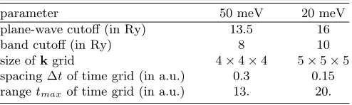
A. Convergence parameters
Before discussing the performance and scaling issues we briefly summarize the results of convergence tests for bulk Si. In Table I the parameters needed to converge quasiparticle energy differences to an accuracy of 50 meV and 20 meV, respectively, with the present method are gathered. This accuracy is meant to be with respect to each parameter individually. We estimate the overall ac-curacy of our results to be better than 0.1 eV. The plane-wave (PW) cutoff in Table I is the cutoff of 12(k+G)2
in the LDA calculation providing the wavefunctions Ψnk.
All PW components of the LDA wave functions are used in theGW calculation. The real-space grids in the unit cell (see Section III B) resulting from PW cutoffs of 13.5 Ry and 16 Ry comprise 9×9×9 and 12×12×12 points, respectively. The band cutoff determines the number of bands included in the band summation in Eq. (3.3) for the calculation of the Green’s function. Band cutoffs of 8 and 10 Ry correspond to taking 109 and 145 bands, re-spectively, into account. For sampling the BZ we employ a regular non-offset grid of k points. The LDA wave-functions are calculated at thekpoints in the irreducible wedge of the BZ. As described in Section III B the dimen-sions of thekgrid in the BZ are equal to the dimensions
(in multiples of primitive lattice vectors)NR
i of the IC,
which must be large enough to comprise the range of non-locality of the Green’s function and the self-energy in Si. The smallerkgrid given in Table I can roughly accomo-date a non-locality range of 14.5 a.u. and the larger of 18 a.u. (−τmax,+τmax) and ∆τ stand for the range and
spacing of the equidistant grid for sampling the functions
F(r,r′, iτ) on the imaginary time axis. The parameters
ωmaxand ∆ωof the corresponding grid in the imaginary
energy domain are related to the time-grid parameters by ∆ω= 2π/(2Nτ−1)∆τ with τmax=Nτ∆τ.
B. Quasiparticle energies for bulk silicon
[image:12.612.68.299.52.134.2]The quasiparticle energies for bulk Si obtained from a well converged calculation with the present method are given in Table II [27]. The LDA calculation was done with the PW pseudopotential method employ-ing a pseudopotential constructed accordemploy-ing to the pre-scription of Hamann [28] and using the Ceperley-Alder exchange-correlation potential [29] in the parametriza-tion of Perdew and Zunger [30]. As can be seen from Table II the calculatedGW quasiparticle energies agree well with quasiparticle excitation energies derived from photoemission, inverse photoemission and optical exper-iments [31–37], except for the position of the bottom of the valence band which appears to be too high in our cal-culation. The agreement of the quasiparticle energy dif-ferences obtained with the present method (GW 1 in Ta-ble II) with those of a recentGW calculation by Fleszar and Hanke [38] is very good. Like us, these authors did not make use of a plasmon pole model to describe the energy dependence of the dynamically screened Coulomb interaction but directly computed its full energy depen-dence.
We investigated how the quasiparticle energies change when the Green’s function is updated by replacing the LDA eigenvalues by the quasiparticle energies and the self-energy recalculated with the updated Green’s func-tion as input, as was done by Hybertsen and Louie [3]. The results (GW 2) are also included in Table II. Updat-ing the Green’s function increases the gap by about 0.1 eV. Now the conduction band energies agree within bet-ter than 0.1 eV with those given in Ref. [3] whereas the valence band energies remain higher by between 0.1 eV and 0.5 eV (relative to the top of the valence band), the difference increasing with the distance of the respective state from the Fermi level.
Indeed, the results of several earlierGW calculations [3,39] are somewhat different from those given in Table II (and Ref. [38]). This can be attributed to the following reasons:
parameter) to be about 0.2 eV too high, as dis-cussed in Ref. [38]; and
(ii) the use of plasmon pole models for the energy de-pendence of the dynamically screened Coulomb in-teraction in the earlier calculations.
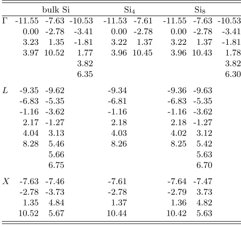
C. Silicon supercells
In Table IV we compare the quasiparticle energies for slab-like Si4 and Si8 supercells to the bulk Si
re-sults. Shown are the quasiparticle energies for the high-symmetrykpoints of Si (which are not necessarily sym-metry points for the supercell geosym-metry) and for those kpoints which are mapped onto these symmetry points when the unit cell size is increased. The calculations were done with a PW cutoff of 13.5 Ry (leading to a real-space grid spacing of ∆r= 0.8 a.u.), a band cutoff of 10 Ry, ∆τ
= 0.3 a.u. andτmax= 20 a.u. Thekgrids have been
cho-sen to make the IC of equal size in all three dimensions for all the calculations, for the reason discussed in Sec-tion III B. The grid sizes resulting from these parameters are summarized in Table III. NIUC, NUC, andNIC are
the numbers of real-space grid points in the irreducible part of the unit cell, the unit cell and the interaction cell, respectively (see Section IV above). Nk stands for
the number ofkpoints in the BZ andNt/ωis the number
of positive time/energy points. The supercell results in Table IV agree with the bulk Si results, as expected. The small differences for the highest conduction band given in Table IV are ascribed to the lower symmetry of the supercells leading to differentGvector sets.
D. Scaling
As outlined in Section IV the computational effort in the present method should scale quadratically with the number of atoms in the unit cell. Fig. 6 shows the CPU times for a fullGW calculation for Sin (n = 2, 4, 8) on
a Digital Alpha 500/500 workstation. The parameters of these calculations are those given in Table III and the discussion thereof. Si2 (bulk Si) has a higher
symme-try than the tetragonal supercells Si4 and Si8. As the
symmetry is exploited in most parts of the calculation this saves approximately a factor of two in CPU time (cf.NIUC values in Table III). Taking this into account
the overall scaling is indeed quadratic, as expected. The most time consuming parts of the calculation are:
(i) setting up the Green’s function according to Eq. (3.3)
(ii) calculating the dynamically screened Coulomb in-teraction (including the inversion of the dielectric matrix [45], the transformation to and from recip-rocal space, and reading ofP0from and writing of
W to disk)
(iii) computation of the matrix elements of the en-ergy dependent self-enen-ergy for a given number of kpoints and bands.
Optionally, the Green’s function can be recomputed when the self-energy is calculated, rather than storing it on disk when it is first set up and reading it in for the calculation of the self-energy. This procedure reduces the required disk space by a factor of 2/3. It has been used for the Si supercell calculations described here. As can be seen from the breakdown of the total CPU time shown in Fig. 6 all these parts of the calculation scale roughly likeN2.
More precisely, the scaling is like NIUCNbands for (i), NIUCNUC for (ii) andNUC2 for (iii) as was discussed in
Section IV.
VII. SUMMARY
We have presented a detailed account of a method for calculating the electron self-energy and related quanti-ties from ab-initio many-body perturbation theory within theGW approximation. The method is based on repre-senting the basic quantities (Green’s function, dielectric response function, dynamically screened Coulomb inter-action and self-energy) on a real-space grid and on the imaginary time axis. In those intermediate steps of the calculation where it is computationally more efficient to work in reciprocal space and imaginary energy we change to the latter representation by means of fast Fourier transforms. Working on the imaginary time/energy axis considerably facilitates the numerical treatment. The matrix elements of the self-energy on the real-energy axis are obtained by an analytic continuation procedure which was shown to be accurate and stable. We have demon-strated the accuracy of the method by calculating quasi-particle excitation energies at high-symmetry points for the prototype semiconductor Si. The computational ef-fort of the method scales quadratically with unit cell size. This was shown explicitly by calculations for Si super-cells. The method allows the extension of ab-initio work beyond the calculation of quasiparticle energies and its application to materials with larger basis sets or larger unit cells than were previously feasible. Calculating the full self-energy gives access to quantities like the charge density [15], spectral function [16], momentum distribu-tion and total energy at theGW level. It also opens the possibility of calculating the self-energy self-consistently and to provide the GW Green’s function (after solving the Dyson equation) – essential prerequisites for going be-yond the GW approximation, e. g., by iterating Hedin’s equations. This remains to be investigated in future.
VIII. ACKNOWLEDGMENTS
We acknowledge helpful discussions with R. J. Needs and A. Rubio. This work was supported by the Engi-neering and Physical Sciences Research Council. M. M. Rieger acknowledges financial support by the European Union under the TMR scheme.
‡ Present address: Siemens AG, Semiconductor Group,
Balanstraße 73, 81617 M¨unchen, Germany. Electronic ad-dress: [email protected]
k Permanent address: Universidad Privada Boliviana,
Casilla 3967, Cochabamba, Bolivia
¶ Electronic address: [email protected]
[1] W. Kohn and L. J. Sham, Phys. Rev.140, A1133 (1965).
[2] M. S. Hybertsen and S. G. Louie, Phys. Rev. Lett. 55, 1418 (1985)
[3] M. S. Hybertsen and S. G. Louie, Phys. Rev. B34, 5390 (1986).
[4] L. Hedin, Phys. Rev.139, A796 (1965).
[5] R. W. Godby, M. Schl¨uter, and L. J. Sham, Phys. Rev. Lett.56, 2415 (1986).
[6] X. Zhu and S. G. Louie, Phys. Rev. B43, 14142 (1991). [7] S. G. Louie, Surf. Sci. 299/300, 346 (1994).
[8] G. Onidaet al., Phys. Rev. Lett.75, 818 (1995). [9] E. C. Ethridge, J. L. Fry, and M. Zaider, Phys. Rev. B
53, 3662 (1996).
[10] H. J. de Groot, P. A. Bobbert, and W. van Haeringen, Phys. Rev. B52, 1100 (1995).
[11] U. von Barth and B. Holm, Phys. Rev. B54, 8411 (1996). [12] E. L. Shirley, Phys. Rev. B54, 7758 (1996).
[13] W.-D. Sch¨one, A. G. Eguiluz and J. A. Gaspar, Bull. Am. Phys. Soc.43, 170 (1998).
[14] B. Holm and U. von Barth, Phys. Rev. B57, 2108 (1998). [15] M. M. Rieger and R. W. Godby, Phys. Rev. B58, 1343
(1998).
[16] H. N. Rojas, R. W. Godby, and R. J. Needs, Phys. Rev. Lett.74, 1827 (1995).
[17] Note that the signs of the exponents and ofτ were given incorrectly in Eq. (3) of Ref. [16].
[18] S. Baroni and R. Resta, Phys. Rev. B33, 7017 (1986). [19] The interaction cell used in the earlier paper, Ref. [16],
was a sphere which slightly exceeded the Wigner-Seitz cell of the IC lattice corresponding to the k-point grid used. Because the use of a discretek-grid imposes an ar-tificial periodicity on the non-local quantities as a func-tion of|r−r′|, this is not optimal. The use of the WS cell in the present paper utilises maximum information while avoiding double-counting arising from the periodicity. [20] X. Blase, A. Rubio, S. G. Louie, and M. L. Cohen, Phys.
Rev. B52, R2225 (1995).
[21] R. W. Godby, M. Schl¨uter, and L. J. Sham, Phys. Rev. B37, 10159 (1988).
[22] M. S. Hybertsen and S. G. Louie, Phys. Rev. B35, 5585 (1987).
[23] R. M. Pick, M. H. Cohen, and R. M. Martin, Phys. Rev. B1, 910 (1970).
[24] We define this quantity as the difference between the GW self-energy and the energy-independent bare-exchange part of the self-energy.
[25] I. D. White, R. W. Godby, M. M. Rieger and R. J. Needs, Phys. Rev. Lett.80, 4265 (1998).
[26] A. Schindlmayr, Phys. Rev. B56, 3528 (1997).
[27] These results are somewhat different from those reported in Ref. [15]. The calculations there still used a spherical cutoff for the interactions as described in Ref. [16], in-stead of the interaction cell defined by thekpoint grid. Tests indicate that the discrepancy arises from the fact that the spherical cutoff in|r−r′|used in Ref. [16] is not
quite consistent with the k-grid used (see Section III B above).
[28] D. R. Hamann, Phys. Rev. B40, 2980 (1989).
[29] D. M. Ceperley and B. J. Alder, Phys. Rev. Lett.45, 566 (1980).
(1981).
[31] Numerical Data and Functional Relationships in Sci-ence and Technology, Vol. 17a ofLandolt-B¨ornstein, New Series, Group III, edited by K.-H. Hellwege and O. Madelung (Springer, Berlin, 1982).
[32] J. E. Ortega and F. J. Himpsel, Phys. Rev. B 47, 2130 (1993).
[33] W. E. Spicer and R. C. Eden, inProceedings of the 9th Int. Conf. on the Phys. of Semicond., edited by S. M. Ryvkin (Nauka, Moskow, 1968), Vol. 1, p. 68.
[34] A. L. Wachset al., Phys. Rev. B32, 2326 (1985). [35] F. J. Himpsel, P. Heimann, and D. E. Eastman, Phys.
Rev. B24, 2003 (1981).
[36] R. Hulthen and N. G. Nilsson, Solid State Commun.18, 1341 (1976).
[37] D. Straub, L. Ley, and F. J. Himpsel, Phys. Rev. Lett.
54, 142 (1985).
[38] A. Fleszar and W. Hanke, Phys. Rev. B56, 10228 (1997). [39] M. Rohlfing, P. Kr¨uger, and J. Pollmann, Phys. Rev. B
48, 17791 (1993).
[40] M. S. Hybertsen and S. G. Louie, Phys. Rev. Lett. 58, 1551 (1987).
[41] J. E. Northrup, Phys. Rev. B47, 10032 (1993).
[42] M. Rohlfing, P. Kr¨uger, and J. Pollmann, Phys. Rev. B
54, 13759 (1996).
[43] M. P. Surh, H. Chacham, and S. G. Louie, Phys. Rev. B
51, 7464 (1995).
[44] E. L. Shirley and S. G. Louie, Phys. Rev. Lett.71, 133 (1993).
[45] Although (ii) forms a major part of the calculation, the inversion of the dielectric matrix itself accounts for only between 2 % (Si2) and 4 % (Si8) of the total CPU time, as
a consequence of doing this inversion in reciprocal space as discussed in Section IV B.
[image:15.612.317.564.569.643.2]FIG. 1. The grids and cells used in the calculation in (a) real and (b) reciprocal space. These are shown here schemat-ically in two dimensions for the case of a 2×2 grid ofk-points (corresponding to an interaction cell of 2×2 unit cells), and a 3×3 real-space grid in the unit cell (corresponding to a 3×3 grid of reciprocal lattice vectors in reciprocal space). The bare Coulomb interaction 1/|r−r′|is non-periodic on the interac-tion cell, and its amplitude at a real-space-grid point is taken to be that at the corresponding point in the Wigner-Seitz cell aroundrof the IC lattice. All other quantities, in both real and reciprocal space, are periodic. In these cases the choice of the primitive (shown) or Wigner-Seitz cell is a matter of computational convenience.
FIG. 2. Fitting of the matrix elements of the correlation self-energyhΣc(iω)iof silicon as a function of imaginary
en-ergy. The real (top panel) and imaginary (lower panel) parts are both reproduced extremely accurately by the fits (which on this scale are indistinguishable from the calculated values). The bands shown are band 1 at the Γ point (solid line for fit-ted and calculafit-ted function), bands 2-4 at Γ (dotfit-ted line), bands 3-4 atX (dashed) and bands 5-6 atX (dot-dashed).
FIG. 3. Convergence of a matrix element (degenerate bands 2-4 at Γ) of the correlation self-energyhΣc(iω)iof
sili-con with respect toωmaxwith a fixed energy grid spacing of
∆ω= 0.16 Har. The top panel shows the calculated self-energy on the imaginary axis with the analytically continued depen-dence on real energy shown in the lower panel. The lines correspond toωmax= 5 Har (dotted), 10 Har (dashed) and
20 Har (solid). Changes in hΣc(ω)i are directly related to
changes in the calculatedhΣc(iω)i, rather than any
instabili-ties in the analytic continuation technique.
FIG. 4. Convergence of hΣc(iω)i with respect to energy
grid spacing ∆ωwith fixedωmax= 10 Har. The lines
corre-spond to ∆ω= 0.24 Har (dotted), 0.16 Har (dashed) and 0.08 Har (solid). As in the previous Figure the analytically contin-ued matrix element converges well, indicating the stability of the fitting procedure. The matrix elements on the real-energy axis (which are obtained in form of fits to a model function, see text) are plotted with a fixed grid spacing of 0.04 Har in order to facilitate comparison between the three curves.
FIG. 5. Real part of a matrix element (degenerate bands 2-4 at Γ) of the correlation self-energyhΣc(ω)ion the real
en-ergy axis, computed withωmax= 5 Har (dot-dashed line), 10
Har (dashed line), and 20 Har (long-dashed line) with fitting
hΣc(iω)ion the imaginary energy axis using the energy range
(−ωmax,+ωmax) and withωmax= 10 Har (dotted line) and
20 Har (solid line) using a fixed energy range of (−5 Har, +5 Har) for the fitting.
FIG. 6. Scaling of the CPU time on a Digital Alpha 500/500 workstation with respect to unit cell size for Sin
(n = 2,4,8). Besides the total CPU time (◦) the times for three major parts of the computation are given: calculation of (i) the Green’s function (2), (ii) the dynamically screened Coulomb interaction (3), and (iii) the matrix elements of the self-energy including a recomputation of the Green’s function (△), see text. Note the quadratic spacing of the abscissa.
TABLE I. Convergence of quasiparticle energies for bulk Si with respect to cutoff and grid parameters in the present method. Shown are the parameters needed for a convergence of 50 meV and 20 meV, respectively.
parameter 50 meV 20 meV
plane-wave cutoff (in Ry) 13.5 16
band cutoff (in Ry) 8 10
TABLE II. Calculated quasiparticle energies at points of high symmetry for Si (in eV). The valence band maximum has been set to zero. The calculation was done with a plane-wave cutoff of 16 Ry, a 5×5×5 k-point grid, a band cutoff of 10 Ry and a time grid with ∆τ = 0.3 a.u. and τmax = 20
a.u. For comparison the eigenvalues obtained in the LDA calculation providing the input for theGW calculation have been included. GW 1 refers to a GW calculation using the LDA Green function whereas in GW 2 the Green function has been updated by replacing the LDA eigenvalues by the quasiparticle energies obtained inGW 1. In the last column some experimental data are given (see text).
band LDA GW 1 GW 2 Experiment Γ1v -11.89 -11.57 -11.58 −12.5±0.6a
Γ′25v 0.00 0.00 0.00 0.00
Γ′15c 2.58 3.24 3.32 3.40a, 3.05b
Γ′
2c 3.28 3.94 4.02 4.23a, 4.1b
X1v -7.78 -7.67 -7.68
X4v -2.82 -2.80 -2.81 -2.9c,−3.3±0.2d
X1c 0.61 1.34 1.42 1.25b
X4c 10.11 10.54 10.63
L′2v -9.57 -9.39 -9.40 −9.3±0.4a
L1v -6.96 -6.86 -6.88 −6.7±0.2a
L′
3v -1.17 -1.17 -1.17 −1.2±0.2a, -1.5e
L1c 1.46 2.14 2.22 2.1f, 2.4±0.15g
L3c 3.33 4.05 4.14 4.15±0.1g
L2c 7.71 8.29 8.39
Egap 0.49 1.20 1.28 1.17a
[image:16.612.52.302.185.387.2]aRef. [31]. bRef. [32]. cRef. [33]. dRef. [34]. eRef. [35]. fRef. [36]. gRef. [37].
TABLE III. Grid parameters for the Sin (n= 2, 4, 8)
cal-culations (see text).
parameter Si2 Si4 Si8
(bulk Si)
NIU C 55 230 455
NU C 9×9×9 9×9×18 9×9×36
Nk 4×4×4 4×4×2 4×4×1
NIC=NU CNk 36×36×36 36×36×36 36×36×36
[image:16.612.54.300.513.599.2]Nt/ω 63 63 63
TABLE IV. Comparison of quasiparticle energies (in eV) at high symmetry points for bulk Si with the corresponding values obtained from calculations for Si4 and Si8 supercells
(see text). All energies refer to the respective valence band top. Shown are the band energies for all k-points mapping onto Γ, X, and L, respectively, when the unit cell size is increased, where those k-points appear in the calculation.
bulk Si Si4 Si8
Γ -11.55 -7.63 -10.53 -11.53 -7.61 -11.55 -7.63 -10.53 0.00 -2.78 -3.41 0.00 -2.78 0.00 -2.78 -3.41 3.23 1.35 -1.81 3.22 1.37 3.22 1.37 -1.81 3.97 10.52 1.77 3.96 10.45 3.96 10.43 1.78
3.82 3.82
6.35 6.30
L -9.35 -9.62 -9.34 -9.36 -9.63 -6.83 -5.35 -6.81 -6.83 -5.35 -1.16 -3.62 -1.16 -1.16 -3.62 2.17 -1.27 2.18 2.18 -1.27 4.04 3.13 4.03 4.02 3.12 8.28 5.46 8.26 8.25 5.42
5.66 5.63
6.75 6.70