MoL 2001 08: Text Categorization and Prototypes

Text Categorization and Prototypes

Alexander Bergo

”There is nothing more basic to thought and language than our sense of similarity; our sorting of things into kinds.”

Acknowledgements:

Contents

1 Introduction 8

1.1 Text Categorization . . . 8

1.2 Two Well-Known Approaches . . . 9

1.2.1 k Nearest Neighbour . . . 9

1.2.2 Rocchio . . . 9

1.3 Our Proposal . . . 10

1.4 Outline . . . 10

2 Two Well-Known Methods in Text Categorization 12 2.1 kNearest Neighbour Classification . . . 12

2.1.1 Computational Concerns . . . 14

2.2 Rocchio . . . 14

2.3 kNN vs. Rocchio . . . 16

3 Prototypes and Dissimilarities 17 3.1 Prototypes . . . 17

3.1.1 Categories and Their Features . . . 17

3.1.2 Categories and Their Representation . . . 18

3.2 A New Approach Based on Dissimilarities . . . 19

3.2.1 Dissimilarity Metrics . . . 21

3.3 Summarizing the Test Scenarios . . . 22

4 Testing the Approaches 25 4.1 The Reuters Collection . . . 26

4.1.1 Format . . . 26

4.1.2 Splitting the collection . . . 27

4.2 Document Representation . . . 28

4.3 Choosing Categories . . . 30

4.4 A Worked-Out Example . . . 30

4.5 Performance Measures . . . 34

5 Results 37 5.1 Results forkNN . . . 37

5.3 Results for Dissimilarities . . . 41 5.3.1 Canberra . . . 44 5.3.2 Minkowski . . . 46

6 Discussion and Conclusion 56

List of Figures

3.1 New tests . . . 23

5.1 kNN graph for cats>2. . . 40

5.2 kNN graph for cats>50. . . 40

5.3 Results for Rocchio. . . 41

5.4 Graph for the mean centroid in the Canberra system. . . 46

5.5 Graphs for Ref. 22, 24, 28 and 32. . . 51

5.6 Graphs for Ref. 40, nrt, 41, nrtII . . . 54

5.7 Best results from mean centroid in Minkowski. . . 55

List of Tables

4.1 Example dictionary. . . 29

4.2 Example documents. . . 30

4.3 Example dictionary. . . 31

4.4 Term frequency matrix. . . 31

4.5 Calculating weights. . . 32

4.6 kNN similarity scores. . . 32

4.7 Rocchio scores. . . 33

4.8 Dissimilarity scores. . . 34

4.9 Process of assignment. . . 35

5.1 kNN, _k1 as category selector. . . 38

5.2 kNN, highest similarity score category selector. . . 38

5.3 Not normalized Rocchio similarities. . . 40

5.4 Normalized Rocchio similarities. . . 41

5.5 Results from the Canberra metric. . . 44

5.6 Internal results for Ref. 2 and Ref. 3. . . 45

5.7 Results form Minkowski for Rocchio prototypes. . . 48

5.8 Internal results for Ref. 15 and 16. . . 48

5.9 Internal results for Ref. 19 and 20. . . 49

5.10 Results from Minkowski for full sets. . . 50

5.11 Internal results for Ref. 21 and Ref. 22. . . 50

5.12 Results for simple mean centroid. . . 52

Chapter 1

Introduction

1.1

Text Categorization

This thesis is about the automated categorization of texts into categories of certain topics. The subject goes at least back to the 1960’s [22]. Since the 1960s we have seen an immense growth in the production and availability of digital libraries, news sources and online documents. As a result, automated text categorization has witnessed an increased and renewed interest.

A generally accepted definition of text categorization is

“Text Categorization (TC) is the task of deciding whether a piece of text belongs to any of a set of prescribed categories. It is a generic text processing task useful in indexing for later retrieval, as a stage in natural language processing systems, for content analysis, and in many other roles.”

Lewis

The core problem in automated text categorization is this: how can doc-uments be assigned to a category with a highest possible chance of being correct without assigning too many incorrect categories, and at acceptable computational costs?

Machine learning paradigm [17, 22] has emerged as one of the main ap-proaches in the area. The machine learning approach to text categorization consists of a general inductive process which automatically builds a classifier based on the characteristics of each of the categories. These characteris-tics are learned from documents already classified and then utilized on the documents to be classified. Advantages of this approach include domain independence and resource saving by focusing on construction of systems instead of the classifier.

theories from other disciplines for TC purposes. More specifically, we will try to improve two aspects which may seem to be at odds with each other: how to achieve a good text categorization system and at a low processing time.

To evaluate the effectiveness of our new methods for document catego-rization, we will compare them to two well-known existing ones: k Nearest Neighbor and Rocchio. Before proceeding, let us briefly recall some details about these methods.

1.2

Two Well-Known Approaches

1.2.1 k Nearest Neighbour

The first approach we will test and use as a basis for comparison is the classic

kNearest Neighbours algorithm (kNN) [17, 15]. This approach has become a standard within the field of text categorization and is included in numerous experiments as a basis for comparison, the main reason being that it is by far the better performing algorithm. kNN takes an arbitrary input document and ranks the k nearest neighbour among the training documents through the use of a similarity score. It then adapts the category of the most similar document or documents;kdenotes the number of neigbours included in the evaluation. As our documents can have more than one category assigned to them, we will try a number of ways of selecting categories from kNN.

Although not perfect, research has shown that kNN is the best overall performing system on diverse sets [9, 32, 31, 11]. In practice kNN compares and ranks each of the already categorized documents with the document to be categorized. This leads, as Mitchell and others [17, 15] points out, to an undesirable amount of computational costs.

1.2.2 Rocchio

To reduce the demand for processing cost we will also implement a centroid1 classifier, called theRocchio classifier. The one we focus on is a well-known information retrieval algorithm developed by Rocchio [14, 24, 26] in the early 1970s, originally to optimize queries from relevance feedback.

This approach makes a centroid document for each category and then ranks the categories, through the use of similarity scores according to which one compares each feature of the category’s centroid document to the fea-tures of the test document. The processing costs are not only reduced, but potentially much lower than forkNN. The higher number of documents that has been categorized already, the bigger the difference in processing costs.

1_{Defined as the point in a system of masses each of whose coordinates is a weighted}

But there are problems because, however good the intentions of using a cen-troid or prototype for each category, the performance is quite poor as we can see in [31].

1.3

Our Proposal

As the discussion so far seems to indicate, there is a basic dichotomy in text categorization between having a good categorizer (kNN) and low process-ing costs (Rocchio). We will try to reconcile the two forces by developprocess-ing centroid- or, as we prefer to call them, prototype-based algorithms that look for similarities anddissimilarities. The basic idea is to measure thedistance between two objects, not the closeness.

In general, our algorithms will consist of two phases:

1. generating prototypes, and

2. comparing documents to be classified to prototypes.

In some settings, however, the two steps will be combined into a single one as seen in [27]. This is done by first measuring the distance between the document to be categorized with the previously categorized documents. The dissimilarity score for each category are then averaged and ranked. The category which has the least average dissimilarity score is adopted to the document we want to categorize.

One of the core issues, then, is to come up with a good notion of pro-totype. We will try to implement notions of prototype that are inspired by fields like psychology, cognitive linguistics and philosophy, mainly by mea-suring dissimilarities between objects. We find the pairwise distance between two objects and then, for each object sub-space, we find the mean distance from the object we want to place in n-dimensional term space and thereby assign a category. The aim is to choose the correct categories for the test documents, by adopting the least dissimilar category. Our approach to dis-tance measuring is based on variations of the so-called Minkowski [12, 8, 33] and Canberra [12, 8] metrics. Among others, we will use these notions of dissimilarity to implement Rocchio prototypes.

Our main aim is to utilize the new approach in such a manner that it possibly can outperform the better approaches in the field today. We will try to utilize methods that perform well, both according to correctly categorizing documents, and to save computation time.

1.4

Outline

Chapter 2

Two Well-Known Methods

in Text Categorization

In this chapter we briefly describe two well-known methods in text catego-rization: k Nearest Neighbour Classification and Rocchio. These are the two methods against which we will compare our own proposals.

2.1

k

Nearest Neighbour Classification

ThekNearest Neighbour (kNN) algorithm is a well-known approach in text categorization. It has been in use since the early stages of TC research, and is one of the best performing methods within the field [31].

The basic idea of thekNN approach in TC can easily be explained: cal-culate a similarity score between the new document and each of the already categorized documents via a data representation model. In this thesis, we adopt a so-called vector space model, where, for each document, each of the words occurring in it is represented by a point in an n-dimensional term space. That is, each document is represented as a vector of weighted word counts, where the weights are relative to the occurrences of the same words in other documents. The documents that have already been categorized are ranked, descending from the document that has the highest similarity score with the document that is to be classified. Ifk >1 we use thektop ranking documents.

Now, what methodology should we use when we choose categories for our unclassified document? In similarity measures we compare a document to other documents that are already categorized. The documents will then be ranked according to their similarity score with the original document. There are basically two ways of assigning a category for our document to be classified;

• or for k >1, that is, if k= 10, then we will include all documents in the ranked list smaller and equal to the document ranked as number 10. We can then use different means of finding a category for our document, including

– sum for the individual categories the score for all the documents in which the category occurs.

– sum for all the categories, the _rank1 in which the category occurs

We will go into greater detail about this at a later stage in this thesis. We note that information about each of the categories score are being extracted from a ranked list of similar documents. These documents are already as-signed a category, and we can adapt categories from the ranked documents in a number of ways.

When there are documents which have the same similarity level there is a tie. To decide if a category is correct the elements from a category are chosen and divided by the number of all elements that have the same similarity score. When using thek-Nearest Neighbours, we need to adjust the impact of the elements relative to their similarity score, so that documents that have a better similarity score will also count more when comparing the different documents in different classes.

Let’s consider an abstract example of categorizing within the kNN ap-proach. A weighted document ~x is to be categorized based on a training set T; we assume k= 1. Determine the similarity score between~x and the elements in the training set~t∈T, and choose all~twhere~t=simmax:

simmax(~x) =max~_t∈Tsim(~x, ~t).

Look for the subset ofT that has the highest similarity with~x.

A={~t∈T |sim(~t, ~x) =simmax(~x)},

let n1, . . . , ni be the number of elements in A that belong to the categories c1, . . . , cifor allci ∈C, respectively. That is,nj =|{d|cat(d) =cj}|. Next,

we estimate conditional probabilities of membership:

P(ci |~x) = ni Pn

i=1ni ,

and we adoptcj ifP(cj |~x)> P(ck |~x) for all kwherek6=j.

Note that the example only takes care of one nearest neighbour. For

2.1.1 Computational Concerns

Let us shortly outline the computational pitfall the above mentioned ap-proach poses; ThekNN approach classifies on the intersection between two documents: it checks the weights occurring in both the unclassified doc-ument and all classified docdoc-uments. That is, it compares each of the test documents with each of the documents in the training set. The bigger train-ing set, the higher computational cost. We will later argue more in detail why this is the case. Now, as earlier research [3, 13, 14, 25, 28] has shown the prototype per category remedy this cost.

2.2

Rocchio

Instead of considering similarity of an unclassified document to all docs in a category, a natural alternative is to somehow take a single representative document per category, called aprototype, and to compare the unclassified document to each of the different category prototypes. At least intuitively, this is bound to save computation if compared to thekNN approach in the previous section.

We will have more to say about prototypes in the following chapter; for now, we will discuss one of the best known prototype based approaches to text categorization: the Rocchio algorithm. Originally the Rocchio algo-rithm was designed for relevance feedback in information retrieval [14, 13]. Retrieving useful documents for a user-query has always been a challeng-ing problem in the field of information retrieval. For optimized retrieval of correct documents there has to be a good categorization. The Rocchio algorithm has been adapted from information retrieval into the field of text categorization.

The basic idea behind applying the Rocchio approach to text catego-rization is to construct a prototype vector for each category. For a given category the prototype vector is the category representative vector of the documents assigned to this particular category. There are a number of dif-ferent approaches to what is considered the optimal prototype vector, and the Rocchio prototype is suggested as one of them. Each weight in the prototype vector is computed by averaging the co-occurring weights from all documents in a given category and subtracting the average of the same co-occurring weights in all documents that do not occur in the category. The result is an efficient method that is relatively easy to implement. The original Rocchio algorithm, as vector-space-model method and relevance feedback algorithm for document routing and filtering in information re-trieval, consists of heuristic components that offer a wide variety of possible implementations [14].

us make things more formal. To be able to express this more formally, we need the following notation:

Definition 1 Learning the Rocchio prototype vector represented as c~k is

achieved by combining each document vector d~j in a given category Ck,

where Ck is the set of documents in category k and then by calculating

the score for each of the co-occurring weights dividing by the number of documents |Ck| in the category. Then subtracting the average score for

each of the weights in the document vectors not in this category,Ck. This

gives the prototype vector~ck [14, 25, 28].

~

ck= (α·)

1

|Ck|

· X

i∈Ck

wik−(β·)

1

|Ck|

· X

i∈Ck

wik. (2.1)

where |Ck| is the number of documents in the category. If an instance in

the prototype vector has a value below 0 it is set to 0.

The α and β in (2.1) are parameters that adjust the relative impact of positive and negative training examples. For our experiments we adopt the settings recommended in [3, 14]: α= 16 and β = 4

Once the prototype for each category has been calculated, the unclassi-fied document is compared with the prototype for each category and thus assigned to the category which has the best similarity score. To avoid pref-erence for larger prototypes we will implement the so-calledcosine similarity between the documents.

Definition 2 For the cosine similarity we use a similarity scoresimbetween two vectors d~ij and c~ik. So sim(d~ij, ~cik) where each of the co-occurring

weights in the vectors are compared. This is denoted by •, which again is defined asPn

i=1(d~ij ·~cik).

sim(d, ~c~ ) = (d~•~c) =

n X

i=1

(d~ij ×~cik),

The unclassified document vector is denoted by d~ij and the prototype

vec-tor is denoted by ~cik. We then turn our attention to how we can look at

similarities where we normalize the vector length. The cosine similarity cos between two vectors d~ij and~cik is defined as

cos(d~ij, ~cik) = ~ dij •~cik

kd~ijk × k~cikk

=

Pn

i=1(d~ij ×~cik) q

Pn

i=1(d~ij)2×Pni=1(~cik)2

All in all, the combination of the two steps just explained (generating proto-types and computing similarity to protoproto-types) makes the Rocchio approach a very flexible and workable algorithm. Whenever a document is categorized, a calculation for each document is not necessary, but only a comparison to the prototype vectors of the available categories. After assigning the new document to a particular category, the prototype for this category is recal-culated. One of the advantages with the Rocchio approach is that there is little need for preprocessing of the data. It is also very computationally attractive compared to many other approaches [24].

2.3

k

NN vs. Rocchio

One of the reasons to why text categorization approaches based on pro-totypes are computationally more attractive than the kNN algorithm can easily be imagined when working with large set of documents. Rather than comparing each new document to every document that is already catego-rized, one only has to compare the new documents to the median document of each category. A database of documents would normally contain more than 10000 documents, and when the amount of documents increase the demand for processing, when using thekNN, would increase proportionally. This leads to an extremely expensive computation. On reasonable small sets of data there would already be a noticeable difference between kNN and Rocchio, with respect to the average computation time used [26].

Chapter 3

Prototypes and

Dissimilarities

In this chapter we describe our own proposal for text categorization, based on an effort to combine the prototype-based ideas that we have already encountered in the Rocchio approach with novel ways to use prototypes in the classification process based on dissimilarity instead of similarity.

3.1

Prototypes

Why do we utilize prototypes? Prototype theory, in linguistics and psy-chology, provides an explanation for the way word meanings are organized in the mind [7, 27, 21, 5]. It is argued that words are categorized on the basis of a whole range of typical features. For example, a prototypical bird has feathers, wings, a beak, the ability to fly and so on. Decisions about category membership are then made by matching the features of a given object against a prototype object where the prototype is said to be the best representative of a category.

Before we delve into our prototype-based approach, we should clarify the nature of a category, its representative prototypes and how we can try to improve already well-known approaches.

3.1.1 Categories and Their Features

the objects are divided into binary oppositional components, stressing the complementary features of the objects in a given category. By stressing the complementary features we indicate that shared features are more important for an object when categorizing it. It is possible to see a document the same way. As an object that contains different meanings, thus being categorized on the basis of binary decisions. However, as Wittgenstein first pointed out, this classical approach does not suffice. According to [33] he mentions in his Philosophical Investigations that the term “game” is defined not by a set of necessary and sufficient features, but by

“a complicated network of similarities overlapping and criss-crossing: sometimes overall similarities, sometimes similarities of detail”

This suggests that a document is to be classified by familiarities, or re-semblance structures. This is later adapted by Rosch [5, 33], and we will use the Roscharian sense of Wittgensteins investigations. The objects of a category do not need to have all features in common. A document that com-pletely lacks any resemblance to a given document in a category, can still be correctly categorized as a member of this category. We need to create a representative that accommodates the demands given by Wittgenstein.

What do these deliberations imply for prototype-based approaches to text categorization? It certainly raises the following question: if we can’t just use the set of all common features as a prototype, what should we use?

3.1.2 Categories and Their Representation

Categorization is a problem cognitive psychologists have dealt with for many years [29]. The basic principle for creating categories are cognitive economy and the perceived world structure. Here, cognitive economy means that the function of categories is to provide maximum information with the least cognitive effort. The principle of perceived world structure means that the perceived world is not an unstructured set of arbitrary and unpredictable attributes. These two principles are directly translatable for us: cognitive economy is nothing but the computational processing costs and world struc-ture is the vector position in then-dimensional term space.

The median representative for a category has been proposed as a suit-able candidate for a prototype within a number of cognitive theories, in-cluding Rosch’s theory of prototypes [33]. Rosch argues that the task for a category system is to provide maximum information with the least effort. Significantly often, there seems to be a common idea used by people when describing the prototype for a category. Moreover, informants were able to describe in great detail the middle-ranking items in a given taxonomy. This led Rosch to the conclusion that these middle ranking objects were the prototypes around which the taxonomies are based.

Rosch’s view was later attacked by, amongst others, Kleiber [33] who claimed that a prototype does not necessarily have to be a real object, but, rather, can be regarded as a mental representation of the best characteristics of a given category. After all, a sparrow, although categorized as a bird, does not define the meaning of bird as such. This indicates that we instead of picking an actual document as the best representative, we compose a document from the documents in the training set which belongs to the given category. Our categories, then, are in need of good informants, that is, a system which can both describe a document and its categories. As we will see later, the TF/IDF weighting scheme is such an informant for the individual documents.

There are, moreover, a few known issues in prototype theory [5, 33] that we need to consider. First, we assume that each category in the prototype theory adopts an idiosyncratic range of criterial features. A problem with this can be to measure distance for documents in the outermost edges of the category. The possibility of having to overcome even more problems are present as our documents sometimes need to be assigned more than one category. Furthermore, decisions about the number and type of features to be included in a prototype are by no means straightforward. And although certain features appear to be more central than others, it has often proved difficult to establish which ones take priority when we make decisions about category membership.

3.2

A New Approach Based on Dissimilarities

and their dissimilarity scores. The second way we will make our prototypes is by applying the Rocchio prototypes in our dissimilarity algorithms. And lastly we will apply a simple mean prototype in the same algorithms. After ranking the dissimilarity scores for each of the later given algorithms we choose the least dissimilar score and assign the category for this document. However in accordance with what we mentioned previously, a member of a category does not necessarily have to have all the quintessential features of a category and this constitutes one of the big problems in choosing an algorithm for making a category representative.

Our underlying assumption is that, when trying to find the similarity score we basically look at the intersection, meaning we calculate only on the weights occurring in both the test and training document. When measuring the distance, we calculate the union between the word weights in two doc-ument, that is, weights which also occur in only one of the documents. Of course, where both the test and the learned object, whether it is a prototype vector or a training vector, have a given weight above zero, one of them will be subtracted from the other and their positive result will be added to the sum of the dissimilarity score. For instance, if we have weightnwhich only occur in the test vector, the value of the weight will be subtracted from the neutral value of the non-existent weight of the prototype vector. However instead of lowering the dissimilarity score we have to add the positive value of the weight. We will choose the category which has the least dissimilar score or the categories which are below a certain threshold of dissimilarity.

We first use the Rocchio vectors but instead of choosing to look for similar features we look for dissimilar features, and, then, by finding the least dissimilar category, we find our match. The promising angle here is that this approach already has a weighted difference between the features of the individual categories and the rest of the categories, thus reducing the number of weights included.

Recall from 2.2 on page 14 that the Rocchio prototype given as

~

ck= (α·)

1

|Ck|

· X

i∈Ck

wik−(β·)

1

|Ck|

· X

i∈Ck

wik

Because the Rocchio prototype is designed first and foremost for similarity measures, we will try to adapt an approach that has been utilized in cognitive psychology by, amongst others, S.K. Reed. He defines the prototype in [27] as

“a prototypeP of a category is the central tendency and can be defined as that pattern which has for each component Xm the

mean value of the mth component of all other patterns in that category.

~ ck=

1

|Ck| X

i∈C ~ di

which is nothing more than a centroid vector ck for category kobtained by

the sum of each co-occurring weightsiin all the documents in the category

kand averaging by the number of documents in the category |Ck|.

We do not modify the prototypes’ relative value in relation to the other categories, as in the Rocchio prototype. The reason lies in that in our distance measurer the thought is to look at all the included weights in the category vector is a crucial factor when we want to find correct categories.

3.2.1 Dissimilarity Metrics

Now that we have decided to use a notion of dissimilarity as part of our text categorization algorithm, the first question is: how do we measure dissimi-larity? In this section we propose two dissimilarity metrics: the Minkowski and the Canberra metrics.

The distance checking is formalized as the Minkowski metric[19, 12, 27] where the intra-dimensional weights are subtractive, and the inter-dimensional weights are additive. By intra-dimensional weights we mean that when we check for the distance between two vectors one of the co-occurring weights are subtracted from the other. The absolute value is then added to the final score, which makes up the inter-dimensional addition.

Djk =

à n

X

i=1

|xij −xik|γ !_γ1

,

where γ ≥1 and Djk is the sum of the dissimilarity between vectors that

have already been classified xk and the vector xj to be classified, for set

of weights i = 1, ..., n. The result will always be positive as we take the absolute value of the difference.

When γ = 1 the algorithm is called Manhattan metric whereas γ = 2 is referred to as Euclidian metric. For values γ > 2 it is referred to as Supermum metric.

In addition to the Minkowski dissimilarity algorithm we will implement and test theCanberra metricwith different realizations thereof. This metric has a simple normalizer. This means for us that for each test document we sum up the difference between the vectors co-occurring weights over the sum of the co-occurring weights [8].

Djk = n X

i=1

|d~ij−c~ik|

(|d~ij|+|cik~|)

whereDjk is the dissimilarity score between vector documentdj and

score will also have to be divided by n to ensure the that the score lies between 0 and 1[12]

Prototypes which have more documents would normally cover a larger term-space area. If we do not normalize the vectors before processing them in our dissimilarity system it would most probably influence the end score for our dissimilarities, and thereby strongly influence the end result for the performance of our system. We aim to reduce the potential influence this has by using a normalization of vector length. We do this so that all vectors have the same influence and possibility to be correctly categorized. We will do this to all vectors, regardless of whether they are document vectors or vectors created from our meta documents, that is prototypes. We will basically focus on two types of vector length normalization. The first way is to convert the vector scores to unit length using the so-called Versor normalization:

~

d= d~i

Pn i=1d~i

Earlier experiments [27, 12, 8] have often focused on a normalization method that differentiates somewhat better on the inter-size of the weights in the vectors and moreover the intra-size, meaning each of the internal weights relative size. This is generally done using the cosine normalization, defined as

~

D= D~w

kD~k

3.3

Summarizing the Test Scenarios

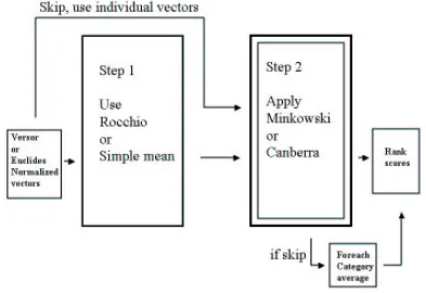
To conclude this chapter we provide a brief overview of the various set-ups and scenarios that we will using for testing later in the thesis. Our main tests will consist of two main processes, as illustrated in Figure 3.1.

In accordance with figure 3.1 we will basically apply three ways of testing the dissimilarity algorithms. Testing is done by way of both the Minkowski metric and the Canberra metric with vectors in n-dimensional term space, that is shown by following the skip pattern in figure 3.1, we will then test the distance by using a prototype derived from the Rocchio algorithm. Lastly we will test by using a simple mean prototype. For all sets we will use a non-normalized set, a versor non-normalized set and a set for the cosine normalization for both test and training set. The Minkowski metric will also be tested with different values forγ. We also check if there are differences in the results for set which include categories with 2≤documents and 50≤ documents.

1. In Canberra metric

• apply Rocchio prototype for

Figure 3.1: New tests

– Versor normalized set

– Cosine normalized set

• skip step 1, use untreated documents, then average end-score for each category for

– untreated set

– Versor normalized set

– Cosine normalized set

• apply simple mean centroid for

– untreated set

– Versor normalized set

– Cosine normalized set

2. In Minkowski metric, and realizations therein,

• apply Rocchio prototype for

– Versor normalized set

– Cosine normalized set

• skip step 1, use untreated documents, then average end-score for each category for

– untreated set

– Versor normalized set

– Cosine normalized set

• apply simple mean centroid for

– untreated set

– Versor normalized set

– Cosine normalized set

Chapter 4

Testing the Approaches

Now that we have presented the basic ideas of our approach to text cate-gorization, the next item on our agenda is to evaluate our approach. As theoretical studies do not provide any indication of the effectiveness of the classification methods and their optimizations, this has to be determined by empirical testing. In any case, empirical testing provides a number of benefits over theoretical complexity. It directly gives resource consumption, in terms of computation time and memory use. It factors in all the pieces of the system, not just the basic algorithm itself.

Empirical testing can be used not only to compare different systems, but also to tune a system with parameters that can be used to modify its performance. Moreover, it can be used to show what sort of inputs the system handles well, and what sort of inputs the system handles poorly. In this chapter we present an outline of our testing methodology.

To be able to test and evaluate our results we need to utilize a set of texts that:

• has the desired format, or at least can be modified into such a format

• can be divided into

– a set for training our systems

– a set for testing our systems performance

• contains enough documents for us to make a reliable assumption and judgement on the performance of our system

• is already categorized relatively well, which will enable us to use the earlier results as a basis for judging the correctness of our tests

4.1

The Reuters Collection

For the evaluation and test of different categorizing approaches we will there-fore use a widely acknowledged [30, 14, 26, 11, 23] and distributed corpus originally used for information retrieval purposes. Namely, the Reuters-21578 collection [16]. In recent years the collection has been modified to fit text categorization purposes.

The documents in the Reuters-21578 collection appeared as Reuters newswire stories in 1987. All the documents are indexed manually and they were made available for information retrieval research purposes in 1990. The files where further modified by D.D. Lewis and Peter Schoemaker and in 1996 a SGML tagged version came as the version with less ambiguity [16]. Lewis and Schoemaker found 595 documents which were exact duplicates of other documents in the set. In addition to the removal of these duplicates, all documents were given a new identifier. The resulting collection is known today as Reuters-21578. The collection is distributed in 22 files, each of the files has 1000 documents except the last which has 578. The documents are formatted with SGML labels to identify the different documents category, title, text, places, people and topics.

4.1.1 Format

There are features in the current version of the Reuters collection that are superfluous for our TC purposes; one can think of features such as the inclusion of topic names, which is directly harmful for the reliability of the experiments. This indicates the necessity for a slight modification of the Reuters-21578 version into a version more suitable for our TC purposes. We deleted unlabelled documents, SGML tags and divided the rest of the documents into a training set and a test set.

The training set was used to create a dictionary. A deeper explanation on this will follow in the following section (Section 4.2 on page 28). We also extracted the topics from the sets, identifying the different documents and their categories as seen in the example later on this section. The latter was done for control purposes for our systems.

The assigned documents have labels like

<TOPICS><D>earn</D><D>acq</D></TOPICS>

to show which categories the document has been assigned. This is an exam-ple document to show how the original documents are structured:

<REUTERS TOPICS="YES" LEWISSPLIT="TRAIN"

CGISPLIT="TRAINING-SET" OLDID="5555" NEWID="12"> <DATE>26-FEB-1987 15:19:15.45</DATE>

<TOPICS><D>earn</D><D>acq</D></TOPICS><PLACES><D>usa</D></PLACES> <PEOPLE></PEOPLE> <ORGS></ORGS> <EXCHANGES></EXCHANGES>

&#22;&#22;&#1;f0773&#31; reutes u f BC-OHIO-MATTRESS-&lt;OMT>-M 02-26 0095</UNKNOWN> <TEXT>&#2;

<TITLE>OHIO MATTRESS &lt;OMT> MAY HAVE LOWER 1ST QTR NET</TITLE> <DATELINE> CLEVELAND, Feb 26 -</DATELINE>

<BODY>Ohio Mattress Co said its first quarter, ending February 28, profits may be below the 2.4 mln dlrs, or 15 cts a share, earned in the first quarter of fiscal 1986. The company said any decline would be due to expenses [...] including

conducting appraisals, in connection with the acquisitions. Reuter &#3; </BODY>

</TEXT> </REUTERS>

To format the documents for TC purposes, we had to re-shape them into a structure where the whole set had a unique document identifier, headline and document body. The headline was made part of the document body. In addition, end-of document markers were inserted.

Here’s an example of such a cleaned-up document:

BEGDOCID_1 OHIO MATTRESS &lt;OMT> MAY HAVE LOWER 1ST QTR NET

Ohio Mattress Co said its first quarter, ending February 28, profits may be below the 2.4 mln dlrs, or 15 cts a share, earned in the first quarter of fiscal 1986. The company said any decline would be due to expenses [...] including conducting appraisals, in connection with the acquisitions.

Reuter ENDDOC

4.1.2 Splitting the collection

Before we could do any experiments, further preparations had to be carried out. For instance, we had to split our collection into documents used for training and for testing. The rules are as follows:

1. we did not use categories (or documents belonging to such categories) which contained at most one document, presuming that the mentioned document only had one or fewer categories assigned to it.

2. we secured that both the training set and test set contained at least one document from each category.

To see if there is a difference in the performance between categories con-taining a small number of documents and categories that contains more documents, we made 2 additional sets. In addition to the split where cat-egories contained 2 or more documents, let’s call it the ”2-split”, we made a set which is split the same way as the previously mentioned set, only this time the criteria for being included is that each of the included categories has to contain at least 50 documents, and the documents have to be a mem-ber of one of these categories. We now have a 2-split and a 50-split. Note that these documents come from the same Reuters-21578 set, but to secure the 80%–20% split we have to randomly redistribute the documents.

In the 2-split set the test set contained in the end 2008 documents. These documents had an average of 1.3 categories assigned to them, that makes 2548 required categories for these documents. There were in fact only 339 documents that have more than one category assigned to them. In the training set there were 7847 documents which also had an average of 1.3 categories. The 50-split set, also has 1.3 categories assigned to each document, on average. The different sets were used to see if the basis for categorization was influenced by the number of documents in the categories.

4.2

Document Representation

To be able to compare the different documents, we transformed them into feature vector representations [10] that is, into vectors of weighted word-counts. We followed the following criteria to extract features from the train-ing documents;

• Punctuation marks are separated from words

• Number and punctuation marks are removed

• All words are converted to lowercase

• Prepositions, conjunctions, auxiliary verbs, articles etc. are removed [23]

• Words are replaced with their morphological root form.

Let’s make the point mentioned above a bit more concrete; words that have the same word-morphology count as the same word, and we chop the affix of the word stems. Words like

economics

and

economy

will have the same representation

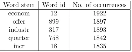
The features derived from our training set of documents were used to create a dictionary containing word stems, word identifiers, and number of times a word occurs in the training set.

Word stem Word id No. of occurrences

econom 12 1922

offer 899 1897

industr 317 1893

quarter 758 1842

incr 18 1835

Table 4.1: Example dictionary.

At a later stage, the dictionary was to be used as a means for calculating the relative importance of the occurrence of words in all documents.

Once the dictionary has been created, the individual document vectors are generated. A vector space model represent documents as vectors of weights inn-dimensional space and this, in fact, constitutes our data repre-sentation model. This method needs little preprocessing of the data, which is a benefit when we are going to process large amounts of data [13]

Definition 3 Term frequency, denoted astfij, is the number of times term ti occurs in documentdj.

Inverse document frequency, the relative occurrence of the termti in the

whole training set, is denoted as idfi = log ³_|N|

ni ´

, where |N|is the number of documents in the training set, andni is the number of documents in the

training set that term ti occurs in.

We determine the weight wij of term ti in document dj by

wij =tfij ·idfi

Thevector for document dj consists of the set of weight from 1 ton as

~

vj = (w1j, ..., wnj)

Earlier research shows that more sophisticated methods of representing the data, although perhaps intuitively more appealing, have performed worse [18], especially when using noun-phrases instead of words [23].

4.3

Choosing Categories

After these preparations, the documents are ready to be compared to other other documents. To find the category that we want to assign to a particular document, we use similarity measures represented by, for instance, thekNN approach, the Rocchio algorithm, or one of our new approaches. Below, we will see an example of how everything is computed. But first we need to show how we select the categories. We use two methods for choosing categories for each test document:

• The first is to simply add the similarity scores from each of the ranked documents to each individual category.

• The second is to, for each of the categories, sum the score of 1/k, wherekis the number rank in the ranked list.

In both approaches the highest scoring category is assigned to the test doc-ument. If there is a tie, then all the tied categories are picked.

Because the documents in our document collection have an average of 1.3 categories assigned to them, we need to make an algorithm that will also select categories that are not the top scoring ones. We could just pick two or more categories from the list, but this would probably lead to worse overall performance since the average number of categories for each document is less than two. The choice of how many categories a document is assigned to is a given percent on the basis of the highest scoring category.

4.4

A Worked-Out Example

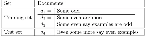
In this section we take a toy document collection and give a fairly detailed account of the way the documents are represented and classified. Suppose we have a set of four documents as given in Table 4.2, where the training set consist of documentsd1,d2,d3, andd4 is our test set. We can see that the split here is 75% and 25%.

Set Documents

Training set

d1 = Some odd

d2 = Some even are more

d3 = Some even say examples are odd Test set d4 = Even some more say even examples

Table 4.2: Example documents.

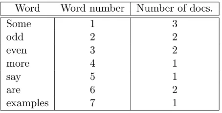
Word Word number Number of docs.

Some 1 3

odd 2 2

even 3 2

more 4 1

say 5 1

are 6 2

examples 7 1

Table 4.3: Example dictionary.

In Table 4.4 our documents are represented in a word occurrence matrix where termti,iterm-identifier anddjdenotes the document,jthe document

identifier.

t1 t2 t3 t4 t5 t6 t7

d1= 1 1

d2= 1 1 1 1

d3= 1 1 1 1 1 1

d4= 1 2 1 1 1

Table 4.4: Term frequency matrix.

The term frequency for each document is listed in Table 4.4; the inverse document frequency of a term is found by the logarithm of the total number of documents in the training set divided by the number of documents in training set whereti6= 0. Note that the vectors in Table 4.4 are not length

normalized; they partly serve as an example of how longer vectors have an advantage over smaller vectors. If these documents had been longer, then the similarity scores would potentially be very high. The method would also favour longer documents as they trivially have more words in them.

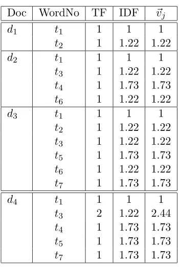
Table 4.5 shows us that the vector~v4, the test document has these values:

~v4 =h1,0,2.44,1.73,1.73,0,1.73i. The default value of a word is 0 so that a word that does not occur just sets the value to 0.

We will pairwise match all document vectors in the training set with our test document vector. It will be done by multiplying the weightsw1, . . . ,w7 for the test document vector~v4 with the co-occurring weights in all the vectors from the training set. By summing up the scores for each of the calculations and rank them according to their score. The comparison that achieves the highest summed score is the document from which our test vector inherits its category. This is thekNN approach.

Doc WordNo TF IDF ~vj

d1 t1 1 1 1

t2 1 1.22 1.22

d2 t1 1 1 1

t3 1 1.22 1.22

t4 1 1.73 1.73

t6 1 1.22 1.22

d3 t1 1 1 1

t2 1 1.22 1.22

t3 1 1.22 1.22

t5 1 1.73 1.73

t6 1 1.22 1.22

t7 1 1.73 1.73

d4 t1 1 1 1

t3 2 1.22 2.44

t4 1 1.73 1.73

t5 1 1.73 1.73

t7 1 1.73 1.73

Table 4.5: Calculating weights.

Doc.Number w1 w2 w3 w4 w5 w6 w7 Result

d4 1 0 2.44 1.73 1.73 0 1.73

d1 1 1.22 0 0 0 0 0

~v4•~v1 1 0 0 0 0 0 0 1

d2 1 0 1.22 1.73 0 1.22 0

~v4•~v2 1 0 2.98 2.99 0 0 0 6.97

d3 1 1.22 1.22 0 1.73 1.22 1.73

~v4•~v3 1 0 2.98 0 2.99 0 2.99 9.96

Table 4.6: kNN similarity scores.

(~v4•~v3)>(~v4•~v2) and (~v4•~v3)>(~v4•~v1) then~v4 will adapt the category of~v3.

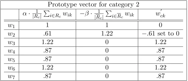
Table 4.7 shows an example of how the Rocchio prototype is computed. For the Rocchio classifier the vectors exists inare given in Table 4.5. The training documents are by definition already classified. Vector~v1 has cate-goryc1 and~v2 and~v3 hasc2 as category. We will compute forc2. Note that we will here use values forα= 1 and β= 1.

w0_ck=α 1

|Rc| X

i∈Rc

wik−β

1

|Rc| X

i∈Rc

Ifcj <0, thencj is set to 0.

For column 2, the weights for c2 are d2 and d3 summed and divided by the number of documents in the category. In column 3 the weight of the rest of training vectors, also called the negative weight, in this case ~v1, is calculated.

Prototype vector for category 2

α·_|R1

c| P

i∈Rcwik −β·

1

|Rc| P

i∈Rcwik w 0 ck

w1 1 1 0

w2 .61 1.22 −.61 set to 0

w3 1.22 0 1.22

w4 .87 0 .87

w5 .87 0 .87

w6 1.22 0 1.22

w7 .87 0 .87

Table 4.7: Rocchio scores.

This calculation would have been done for all the predefined categories. The similarity would then have been computed the same way as for the kNN, however instead of using the vectors from the training set, we would utilize the new prototype vectors.

Now our attention moves to dissimilarities. We already have the vectors from table 4.5. One of our new classifiers, the Minkowski Metric will be exemplified here. The goal is to find the least dissimilar category for each of the test documents. We have talked about two basic ways of computing dissimilarities (see illustration in section 3.1 on page 23):

1. For each of the documents in the training set, compute the average dissimilarity for each of the categories by first measuring the distance between the test vector and all the training vectors and then average the distance for each of the categories.

2. First make a prototype for each of the categories, and then compute the dissimilarities

We go for the second option. Assume the mean centroid,

~

C = 1

|R| X

t∈R ~ d,

which, for categoryc1 is trivially the same asd1, as there is only one docu-ment in this category. Forc2 the average score for the weights in the vectors

of documents in this particular category.The values for the weights is the values forw1, . . . , w7 in the second column in Table 4.7.

For the Manhattan metric we look for the least dissimilar prototype:

min

i { n X

w=1

|d~4−c~i|}

We also need dissimilarities between the vector for document 4,~v4 and the simple mean centroid vector for category 2, C~2 is smaller than the dissim-ilarity between vector for document 4,~v4 and simple mean centroid vector for category 2,C~1, thus category 2 is assigned tod4.

Doc. No. w1 w2 w3 w4 w5 w6 w7 sum diss.

d4 1 0 2.44 1.73 1.73 0 1.73

c1 1 1.22 0 0 0 0 0

~v4•~c1 0 1.22 2.44 1.73 1.73 0 1.73 7.12

c2 1 .61 1.22 .87 .87 1.22 .87

~v4•~c2 0 .61 1.22 .87 .87 1.22 .87 5.66

Table 4.8: Dissimilarity scores.

An example for the Canberra metric would not look very different in this case. Each of the dissimilarity scores would be the average dissimilarity score between two weights.

In conclusion, we have seen that all of our systems will categorize docu-ment 4 in category 2.

4.5

Performance Measures

The conclude this chapter, we discuss the performance measures that we will use in our experiments.

After computing similarities and dissimilarities we need a method for measuring the correctness of our findings. The primary goal is not only to find the categories originally assigned to the test documents, but also to not include categories which are not assigned to the test documents originally. To be able to reliably measure the performance of the different systems, we use widely accepted methods for measuring [31]:

• precision

• recall

These will be explained shortly.

For each document we look for categories to assign, also called category ranking. Each of our classification algorithms returns, for each of the test documents in the given test set, a ranked list of categories; recall and pre-cision can then be computed at any threshold on this ranked list. We can classify the categories above threshold four ways. For binary classifiers a two-ways contingency table for each category is used to evaluate the assign-ments. The conventional performance measures as recall and precision are defined and computed from this table. They are calculated for each of the categories where the category has a document which is a member of the test set.

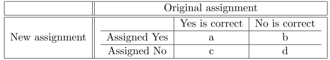
In Table 4.9 the correctness of how the test documents are assigned, or have categories assigned to them are counted in relation to the original assignment.

Original assignment

New assignment

Yes is correct No is correct

Assigned Yes a b

Assigned No c d

Table 4.9: Process of assignment.

Here

• cell a counts categories correctly assigned to the test set

• cell b counts categories incorrectly assigned to the test set

• cell c counts categories incorrectly rejected from the test set

• cell d counts categories correct rejected from the test set

From these scores we calculate the recall, precision and f-score, in the fol-lowing manner:

Recall = a a + c,

where we assume a+c >0, otherwise recall is undefined. Recall measures the algorithm’s performance relative to the original assigned documents. For instance, if there are 2000 categories originally assigned to the different test documents, and the given approach has 1500 categories correctly assigned to the test set, then our recall score will be .75. By itself this may seem like a reasonable score, but if these 1500 correct categories comes from 9000 categories assigned all together, then the score is not impressive.

Therefore the precision measure is introduced.

where we assume a+b > 0, otherwise precision is undefined. Using the example mentioned above, this would give us, from the 9000 assigned cat-egories, where 1500 were correctly assigned, a precision score of .16. This score indicates that although we found a lot of correct categories, we picked too many. Moreover it indicates that if we only examine the recall it might be somewhat misleading.

Recall and precision scores usually exhibit a trade-off in the classifier, when adjusting parameter internally. We would like to find a score which gives us one score from the precision and recall score. If we use interpolated “break-even point” (BEP) [31], which is the average of the precision and recall score, then the BEP will not always reflect the true behaviour of our classifier. That is, if the precision and recall score are far apart, as our example, we do not think of.46 as a reasonable performance for our system. To find a single numbered measure that more accurately reflects what we think is correct we turn to Van Rijsbergen’sf-score [31].

f-score = ₁ 2

recall + precision1

.

Chapter 5

Results

In this chapter we present our experimental results. We start out but set-ting the baseline scores, by looking at the kNN and Rocchio classifiers. After that, in Section 5.3, we present results obtained using systems based on dis-similarities. To help the reader keep track of the many options we consider, a brief overview at the start of Section 5.3.

5.1

Results for

k

NN

Picked categories. For kNN we chose categories from the ranked list two ways as we mentioned in Chapter 3 on page 17. The first way to assign categories is the 1_k. The results are seen in Table 5.1 on page 38. This way of finding the appropriate category adapts each of the categories for the chosen

knearest neighbour documents. Then simply sum, for each category, all the 1

k values from the ranked training documents, where the category rank is

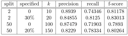
represented. k is the rank from the similarity scores. In practice this will mean for k = 4, that if the 1 nearest neighboring (k = 1) document has ”lead” as the category, and the correct category is “grain”, then the next three training documents will have to have “grain” as one of their categories to be able to correctly assign grain to our test document as 1₂ +1₃ +1₄ > 1₁. The category(ies) which has the best scores will be assigned to the document. The results shows that the 2-split set peak for the f-score at k = 10. The f-score is here 0.81178. The precision is here 0.8939 whereas the recall is 0.74. This may indicate that many of the found documents are correct, but that we should try to pick more categories. This is done by looking at the final best scoring category, and then by looking for categories that performed almost as good as the best scoring category.

documents found and correctly assigned. To remedy, or more precisely to check, if there is a significant difference in kNN’s ability to classify with a higher probability of correctness when the categories have a minimum of 50 documents we utilize the 50-split. Different approaches perform comparably when categories are sufficiently common [32].

split specified k precision recall f-score

2 0 10 0.8939 0.74346 0.81178

2 30% 20 0.84855 0.8125 0.83013

50 0 100 0.87479 0.71903 0.7893

50 20% 150 0.8229 0.78334 0.80264

Table 5.1: kNN, 1

k as category selector.

In Table 5.1 and Table 5.2, column one denotes from which set the results come. Second column is what kind of percent frame was used to choose categories relative to the top-scoring category. 0 denotes that only the top scoring category has been chosen. The column labelled withkindicates how many nearest neighbours that were used.

The same way that we showed the scores for 1

k we display the scores for

the categories chosen by summing the similarity scores for each of the cate-gories represented in the ranked training vectors. Highest scoring category, as seen in Table 5.2 is assigned to the document. If there is a tie, all the categories in the tie will be assigned to the document.

split specified k precision recall f-score 2 flat 8 0.8896 0.74429 0.8105

2 20% 8 0.85733 0.7953 0.8252

50 flat 75 0.88632 0.7285 0.7997

50 10% 75 0.8483 0.761 0.80228

Table 5.2: kNN, highest similarity score category selector.

This approach (Table 5.2) seems to be performing just as well as the 1_k ap-proach. However, the performance decreases relatively rapid ask increases. An example of the decrease is illustrated by the graph in Figure 5.1. This is probably due to the fact that the Reuters collection has 27 (not including the 18 categories that only contain one or no document) categories which has five or less documents in them. This will inevitable affect results whenk

We have seen that one of the problems for kNN is that our documents are not supposed to have only one category. It is not necessary to choose either this or that category, it may be that both are correct. As indicated we tried to include the top scoring category and the categories that has a score which is almost as good. We did this by including categories that did not differ more than a given percentage from the top-ranked category score. This approach shows, as seen in Table 5.2, a score of about 2−3% better than to pick only the top scoring category. It has a best f-score of 0.83 for 30% diversion, weightedk= 2. The problem is that this particular matrix shows signs of fluctuation compared to 1

k approach also for 30%. This has

a top score of 0.83 for k = 20. What is interesting is that the lowest score for this approach is 0.8, which is about 0.06 better that the lowest scoring 30% weightedk. This, of course, has to be included when making a decision about which approach is preferred in the end.

When looking at the graphs in Figures 5.1 and 5.2, it is evident that the set containing two or more documents per category performs slightly better than its opponent here. However, the better performance is at a lower value for k, and the set where each category has fifty or more documents seem overall to be performing more steadily.

This experiment shows an important development in that it seems to indicate that as the minimum number of documents per category increases, the number of neigbours that has to be included in the similarity score increases. For the test set where there are two documents or more per category, we see a slight decline in performance as the number of neighbours increase.

5.2

Results for the Rocchio prototype

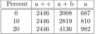
The Rocchio algorithm is designed to first create a prototype representative per category, and then rank these representatives according the similarity scores. Then adapt the most similar category to the test document. As expected the best results came when choosing only the most similar category. It has an f-score of.3. However if when we look a bit deeper into the results it seems like the Rocchio is distinguishing quite well between the different super-categories [16]. When we perform a vector length normalization on the prototype it self, we note an overwhelming increase in performance as seen when comparing the graphs in Figure 5.3.

For the prototypes we select categories by assigning the best similarity score and the scores relative to that score.

0 25 50 75 100 125 150 175 0.7

0.75 0.8 0.85 0.9

Number of k

score

30% cat > 2 flat cat > 2

Figure 5.1: kNN graph for cats>2.

0 25 50 75 100 125 150 175

0.7 0.75 0.8 0.85 0.9

Number of k

score

10% cat > 50 flat cat > 50

Figure 5.2: kNN graph for cats>50.

Percent a + c a + b a

0 2446 2008 687

10 2446 2819 810

20 2446 4136 982

Table 5.3: Not normalized Rocchio similarities.

normalized set evaluated.

Percent a + b a Rec Prec f-score

0 2578 1480 .61 .57 .58

10 6289 1926 .79 .31 .44

20 15262 2126 .87 .13 .24

50>0 2542 1447 .64 .57 .60

Table 5.4: Normalized Rocchio similarities.

large set. By large category we here mean well over 100 documents. The reservation lies, for us, in the incomparable results this test showed as it computes the accuracy instead of computing precision and recall. Comput-ing accuracy has pitfalls for sets where the number of categories are large and the number of documents per category is low.

The difference between normalized set and an unmodified prototype is illustrated graphically in Figure 5.3.

0 10 20 30 40 50 60

0 0.1 0.2 0.3 0.4 0.5 0.6 0.7 0.8 0.9 1 Percent score UC f−score UC precision UC recall

0 10 20 30 40 50 60

0 0.1 0.2 0.3 0.4 0.5 0.6 0.7 0.8 0.9 1 Percent score Cos f−score Cos Precision Cos Recall

Figure 5.3: Results for Rocchio.

Regarding the coding in Tables 5.3 and 5.4 and the graphs in Figure 5.3 we note that Table 5.3 has not been normalized, whereas Table 5.4 has been cosine normalized. From the graph we can see that, as expected due to the average number of categories in the test set being 1.3, the Rocchio algorithm has its best performance when we only pick the best scoring categories. The result also provides strong indications that it is necessary to normalize the similarity scores due to the noise introduced by the prototypes internal size difference.

5.3

Results for Dissimilarities

scores, not only the better performing ones. These results can serve well to explain the nature of the selection process and in what way the better performing algorithms are successful in choosing categories for the different documents representation sets. First we have a closer look at the results for the Canberra algorithm. Due to the incorporated normalization we also tested it for a non-normalized set.

Note that the method for choosing more categories are basically the same as for the kNN approach. For each of the test documents we choose categories in the ranked list by their score relative to the least dissimilar score. It is, however, useless to select by including via the rank as the categories themselves are ranked. If we were to include more categories, based on the rank, we would always get the same number of categories for each of the test documents. Due to the nature of the dissimilarity scores we choose not to increase by 10% at the time but by 1%.

The tables consist of columns where

• “set” is the explanation of what set we tested the algorithms

– “All” conveys that all the vectors from the training set are used as basis for comparison, and the prototype is then calculated as described in Figure 3.1 on page 23

– “Roc” is then that the system use the Rocchio prototypes as basis for comparison

– “Ctr” denotes results from the purely mean Centroid vectors

• “nrm” describes if we used document length normalization and which one we used. These are coded as

– “NoN” is sets where no document length normalization has been applied

– “Ver” denotes the Versor vector size normalization

– “Ecl” indicates that we have a set normalized by the Euclides vector size normalization

• “Ref” is this particular result reference number for referral later in the text

• “split” explains how many documents there was in each per category for the category to be counted as valid.

• “Rec” is the recall

• “prec” is the precision

• for the Minkowski metric we also include %/R. It denotes the per cent or number of Ranking (R) that are included in the results the same way as for the Rocchio similarity score

• we also include a value forγ, as given in the formula 3.2.1 on page 3.2.1, which is the variable included in the algorithm.

For the dissimilarity score for the new prototypes we have also looked into the performance the system had on the ranking of individual categories. The reason to this was that we needed more information on how, and why the metric performed. We evaluated, for 4−6 different categories, the aver-age rank in documents that were supposed to have the particular category above threshold for selection and compare them to the average rank for the categories for documents where they are not supposed to be above threshold. These categories are fundamentally different in that they contain everything from 2 to over 700 documents. This is a potentially crucial point in that some of our systems might prefer smaller or larger categories. We will also see details of how the size of the categories included in the test set can influence the performance.

The results for these tests are tables where

• “Categ” denotes the category that are measured and the mentioned categories are:

– “lit”

– “austdlr”

– “ipi”

– “alum”

– “money-supply”

– “acq”

– “earn”

• “a+c” is the number of documents in the test set that are supposed to have the particular category assigned to it

• “avr. for a+c” is the average rank the category in fact had when it was supposed to be assigned to the test document

• “avr. for rest” is the average rank the category had when it was not supposed to be assigned to the test document

5.3.1 Canberra

First, we have tested the Canberra metric and compared all the weights in the test-set vectors with the weights in training-set vectors, and then averaged the dissimilarity scores for each category.

CANBERRA MEASURES

Set Nrm. Ref. Cat a Rec Prec f-scr

All NoN 2 2 9 0.004 0.004 0.004

3 50 1022 0.45 0.51 0.48

Ver 4 2 10 0.004 0.005 0.005

5 50 942 0.417 0.47 0.44 Ecl 6 2 10 0.004 0.005 0.005

7 50 956 0.42 0.48 0.45

Table 5.5: Results from the Canberra metric.

In Ref. 2 we use an unweighted set and we note that the performance gives no grounds for optimism. But if we look a bit deeper below the surface we can see that Ref. 3, from the same dissimilarity scores as 2, only here we used the 50-split, the system suddenly finds over a thousand correct categories. For Ref. 4 and 5 we have the Versor normalization, and we observe that the same way as Ref. 2 and 3 it performs better when only including categories with fifty or more documents in them. The first issue we notice is the enormous difference between the f-scores for the dissimilarity scores where the categories which has over 2 documents per category and over 50 documents per category are included. In fact if we look at Ref. 2 we can see that it has an impressive lack of ability to choose the correct categories. Compared to Ref. 3, which are test done in the same context, but with the 50-split. The correctly assigned documents increase by over 1000. This may suggest that, as this is a test done on a non-normalized set, the Canberra metrics built in normalizer works to a certain degree, but that it, as expected might not be a very good length normalizer. The same goes for sets that are Versor normalized (Ref. 4 and 5) and Cosine normalized (5 and 6). Mind you, these scores are done on sets where we average the sum of the individual document dissimilarity scores for each category.

per category.

The results from Ref. 2 and 3 were not normalized before the test. Whereas the result for Ref. 2 has an amazingly poor performance at 0.004, the result for Ref. 3 is better. Not very good, but there is a significant dif-ference compared to Ref. 2. If we look at the internal results from the same categories as mentioned above, we immediately locate a possible reason, namely interference from categories that has fewer documents in them.

Note that the assumption is that categories containing more documents, in general, has more weights.

Catg. a+c avr. for a+c avr. rest

lit 1 1 9.4

austdlr 1 2 2.22

ipi 8 33.75 57.7

alum 13 45.08 57.19

money-supply 22 34.14 66.93

acq 449 51.82 74.78

earn 709 31.55 77.73

made for Ref. 2.

ipi 8 1.38 10.39

alum 13 3.39 8.91

money-supply 22 2.41 18.82

acq 449 6.62 26

earn 709 4.59 28.94

made for Ref. 3.

Table 5.6: Internal results for Ref. 2 and Ref. 3.

The categories “lit” and “austdlr” have either 1 or 2 documents in the test set. All in all the category austdlr has 3 documents in it, which means that there are only 1 or 2 documents in the training set. For Ref. 2 it correctly assigns the category to the correct test vector, however it seem like the extremely low number of documents in it affects the rest of the categorization task. It is probably due to the fact that the dissimilarity measures on all the weights. That makes it vulnerable to categories with few number of weights in them. By not using categories which has less than 50 documents increases the correctly assigned documents by 950 (Ref. 3) strongly supports this hypothesis.We can also see the consistency in being vulnerable to categories that contains fewer weights in them by looking at the relations between Ref. 4 and 5 and Ref. 6 and 7 respectively. They have different document length normalization, but still the same phenomena occurs.