End to end model of Icelandic waters using the Atlantis framework: exploring system dynamics and model reliability

Contents lists available atScienceDirect

Fisheries Research

journal homepage:www.elsevier.com/locate/fishres

End-to-end model of Icelandic waters using the Atlantis framework:

Exploring system dynamics and model reliability

Erla Sturludottir

, Christopher Desjardins

, Bjarki Elvarsson

, Elizabeth A. Fulton

,

Rebecca Gorton

, Kai Logemann

, Gunnar Stefansson

a_{Science Institution, University of Iceland, Taeknigardur, Dunhagi 5, 107 Reykjavik, Iceland} b_{Marine and Freshwater Research Institute, Skulagata 4, PO Box 1390, 121 Reykjavik, Iceland} c_{CSIRO Oceans and Atmosphere, Hobart, Tasmania 7001, Australia}

d_{Centre for Marine Socioecology, University of Tasmania, Battery Point, 7004 Tasmania, Australia} e_{MARICE, Faculty of Life and Environmental Sciences, University of Iceland, 101 Reykjavik, Iceland}

A R T I C L E I N F O

Handled by A.E. Punt

Keywords:

Atlantis Ecosystem model Icelandic waters Sensitivity analysis Skill assessment

A B S T R A C T

Icelandic waters are very productive and thefisheries are economically important for the Icelandic nation. The importance of thefisheries has led to progressivefisheries management and extensive monitoring of the eco-system. However,fisheries management is mainly built on single species stock assessment models, and multi-species or ecological models are essential for building capacity around ecosystem-basedfisheries management. This paper describes thefirst end-to-end model for the Icelandic waters using the Atlantis modeling framework. The modeled area is 1,600,000 km2_{, and covers the area from Greenland through Icelandic waters to the Faroe} Islands. The ocean area was divided into 51 spatial boxes, each with multiple vertical layers. There were 52 functional groups in the model: 20fish groups (8 at a species level), 5 groups of mammals, 1 seabird group, 16 invertebrates, 5 primary producers, 2 bacteria and 3 detritus groups. The reliability of the model was evaluated using a skill assessment and a sensitivity analysis was conducted to understand the dynamics of the system. The sensitivity study revealed that saithe, redfish and tooth whales had the greatest effect on other groups in the system. The skill assessment showed that the model was able to replicate time-series of biomass and landings for the most important commercial groups and that modeling of the recruitment processes was important for some of the groups. This model now provides a solid basis for evaluating alternative ecosystem andfisheries man-agement scenarios, and should produce reliable results for the most important commercial groups.

1. Introduction

Icelandic waters, where the relatively warm Atlantic water and the cold Arctic water meet, are very productive (Astthorsson et al., 2007). The annual harvest from these waters is around 1.3 million tones, which is 1.4% of the world´s harvest (Statistics Iceland, 2017). The fisheries are economically important for the Icelandic nation and they have, along withfish processing, accounted for 6–11% of the GDP and 37–63% of the exports since 2002 (Statistics Iceland, 2017). The highest catches are of capelin (Mallotus villosus), but cod (Gadus morhua)has the highest commercial value.

The importance of the fisheries has led to progressive fisheries management, and Iceland was one of thefirst nations to implement a quota system (Hilborn, 2007; Matthíasson, 2003). The ecosystem monitoring program is extensive and a bottom trawl survey is carried out twice annually (Anon., 2010) while acoustic surveys are conducted

for pelagic species (Anon., 2016;Vilhjálmsson and Carscadden, 2002). The environmental conditions around Iceland are also monitored an-nually where nutrients, temperature, salinity and plankton is measured (Anon., 2015). In spite of extended datasets, including data on stomach contents,fisheries management advice is mainly built on single species stock assessment models for the most important commercial species (Anon., 2016). Nevertheless, there has been increased demand for ecosystem-basedfisheries management (EBFM) in recent years. Single species models do not consider species interactions, which are an im-portant factor in EBFM (Link, 2002). Multi-species and ecosystem models, where species interactions, and in some cases environmental factors, are considered are tools that can be used to support EBFM (Plagányi, 2007). Two preliminary food web models have been built for Icelandic waters (Buchary, 2001; Mendy, 1998), but have not been tested or used forfisheries management. A dynamic ecosystem model could support an EBFM and allowfisheries scenarios concerning the

https://doi.org/10.1016/j.fishres.2018.05.026

Received 27 February 2018; Received in revised form 29 May 2018; Accepted 30 May 2018 ⁎_{Corresponding author.}

E-mail address:[email protected](E. Sturludottir).

most important commercial groups, e.g. the effects of stopfishing ca-pelin, an important prey species in the system, to be evaluated.

Modeling of marine ecosystems has increased in recent years, with developments in computational power, along with a growing under-standing of ecosystem functioning and increased data sampling (Fulton, 2010). End-to-end models have become possible, where ecosystem and human components are integrated. They are not appropriate for tactical management advice (e.g., quota setting), unlike the single species models, but are useful to evaluate system-level trade-offs of alternative management strategies. Ecopath with Ecosim (EwE), a trophically-fo-cused ecosystem model, has become widely used (Christensen and Walters, 2004;Fulton, 2010), but more complex models such as Atlantis are becoming more widely used (Fulton, 2010; Fulton et al., 2011; Nyamweya et al., 2016;Ortega-Cisneros et al., 2017).

Atlantis (Audzijonyte et al., 2017a,2017b;Fulton et al., 2011) is a spatially resolved deterministic end-to-end model designed for exploited marine ecosystems. The modeling framework consists of four sub-models: biophysical,fisheries, management and socio-economic. It has been used to explore major processes and responses in systems (Kaplan et al., 2014;Nyamweya et al., 2016) and it has been used for management strategy evaluations (MSE,Fulton et al., 2007).

Different ecosystem models (e.g. Atlantis vs. EwE) for the same areas are not always consistent and have shown contradicting predic-tions (Forrest et al., 2015;Pope et al., 2018). Such an ensemble mod-eling approach can provide major insights into uncertainty around system structure and function. This is important as the modeling pro-cess for these models is subjective, as formal parameter estimation is prohibited by the complexity of the models. Instead, they are currently typically manually calibrated to historical data. This source of potential uncertainty means that even when not being used in an ensemble, a model skill assessment is an important means of determining how re-liable models are, i.e. how well theyfit to existing data and how well they predict (Olsen et al., 2016). The prediction ability of models is however usually not assessed because all existing data are used to ca-librate the model (with subsequent use focused on relative projections rather than focusing on absolute predictions). Olsen et al. (2016) however performed a skill assessment on the predictive capacity of the Atlantis model for the northeast US, ten years after the calibration,

when new data had been acquired. They recommend using a several metrics to assess the different aspects of the skill of the model, e.g. one that measures correlation and another that measures scale mismatch. They concluded that the forecasting skill of the model for the northeast US was comparable with the hindcasting skill, and did not degenerate for a medium-term forecasting.

Finding means of assessing uncertainties and performance for large ecosystem models is important, as they have both inherent structural and parametric uncertainty. Unfortunately, their size has meant tradi-tional approaches to assessing parametric uncertainty (let alone struc-tural uncertainty) have been impractical due to the curse of di-mensionality, rapid growth of complexity in multi-parametric analyses and sensitivity to experimental design due to the feedback influences on time dependence of parametric sensitivity results (Fulton, 2010;Fulton et al., 2011). A sensitivity analysis can give insight into which para-meters contribute the most towards uncertainty in the output (Pantus, 2007;Saltelli et al., 2006). However, a complete sensitivity analysis is not feasible for Atlantis because it has thousands of parameters and numerous possible interactions. Therefore, sensitivity analysis of Atlantis models have been carried out for each parameter one-at-time (Murray and Parslow, 1997) or for interactions between a selection of parameters, which are already known to have a strong influence on model performance or are particularly pertinent to that system type (Ortega-Cisneros et al., 2017).

This paper describes thefirst end-to-end model for Icelandic waters using the Atlantis modeling framework. The aim with this work is to describe the model, compare its output to available data and evaluate its reliability using a skill assessment. The aim is also to investigate how sensitive the output is to changes in parameters and to use a partial sensitivity analysis to understand the dynamics of the system.

2. Material and methods

2.1. Study area

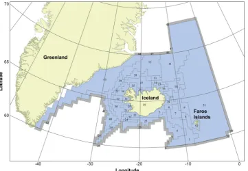
The study area, the Icelandic waters, extends from 60° to 73°N and from 43° to 0°W (Fig. 1). Two water masses meet in this area, the re-latively warm and saline Atlantic water and cold Arctic water with low

Fig. 1.The modeled area and the locations of the 53 spatial boxes. Active boxes are in blue and boundary boxes in grey. (For interpretation of the references to color

salinity (Astthorsson et al., 2007). The mixing of these two water masses causes rather unstable environmental conditions, which has a substantial impact on the production of the lower trophic levels (Gislason et al., 2016). Primary production is higher in the warm Atlantic water south of Iceland than in the cold Arctic water to the north and east of the island (Astthorsson et al., 2007). This has an impact on both the productivity and distribution of thefish stocks. The main spawning grounds of the most important commercial species are in the warm water to the south while the nursery grounds are in the colder water to the north (Astthorsson et al., 2007). Around 30 fish species and seven invertebrate species are commercially harvested in Icelandic waters, along with whales and seals (Anon., 2016). The most important commercial species is cod because of its high catches and commercial value. Another importantfish stock is the capelin, being the most abundant pelagic stock in Icelandic waters and an important prey for many demersal species such as cod, saithe (Pollachius virens) and Greenland halibut (Reinhardtius hippoglossoides). Capelin feed in the northern most part of the area and transfer large amount of energy to the more southern grounds with their feeding and spawning migrations (Vilhjálmsson, 1994). Over 20 species of mammals inhabit Icelandic waters where they have great influence on the ecosystem; it has been estimated that marine mammals consume over 6 million tons offish, cephalopods and zooplankton annually (Sigurjonsson and Vikingsson, 1997). Icelandic waters also support large populations of seabirds (Lilliendahl and Solmundsson, 1997).

2.2. Model structure

2.2.1. The oceanography model

The modeled area is 1,600,000 km2 _{and covers the area from} Greenland through the Icelandic waters and to the Faroe Islands (Fig. 1). The area has been divided into 51 ocean boxes and two land boxes based on work described inStefánsson and Palsson (1997)and in Taylor (2005)where the division was mainly based on hydrography, bathymetry and species distribution. Areas outside of the survey cov-erage are divided into larger boxes because of less information on species distribution. Active boxes (where the biology was modeled) numbered 36, with an additional 15 boundary boxes to buffer water fluxes to and from waters beyond the model domain. Each box was further divided into vertical layers depending on the depth of the box. The boxes each have one sediment layer and can have a maximum of six water column layers (0–50 m, 50–150 m, 150–300 m, 300–600 m, 600–1000 m and 1000 m+). The oceanographic data were taken from a hydrodynamic model (Logemann et al., 2013) and waterfluxes, tem-perature and salinity were calculated for each box and layer each day to create a forcing time series running from 1948 to 2012. A full model run is therefore 65 years and the time step of the model is 12 h. 2.2.2. Biological model

There were 52 functional groups in the model: 20fish groups (8 represented at a species level), 5 groups of mammals, 1 seabird group, 16 invertebrates, 5 primary producers, 2 bacteria and 3 detritus groups (Tables 1 and 2). The vertebrate groups could have up to ten age classes, each of which could contain multiple annual cohorts. The model tracks numbers and weight (mg N) per age class and the weight was divided into reserve and structural weight, where reserve weight was soft tissues and structural weight the bone structure. Cephalopods and shrimp have two age classes, juveniles and adults. Other groups were represented as aggregate biomass pools with no explicit age structure. The initial conditions of most of the vertebrate groups, i.e. their biomass and weight per individual were acquired from data sampled by the Marine and Freshwater Research Institute (MFRI) or from reports from the Institute (Anon., 2016). Initial condition for zooplankton and primary producers were acquired from Astthorsson et al. (2007).

The consumption rate of preyiby predator j(CRij) was modeled

Table 1

The vertebrate groups: the group code, group name and species, their maximum age, reproduction function (BH = Beverton-Holt, BH-f = Beverton-Holt with recruitment scalars, C = constant per adult), if the group is being harvested and if a group is migratory.

Code Group Max age Reprod. Harvest. Mig.

FCD Cod (Gadus morhua) 20 BH-f Yes No

FHA Haddock (Melanogrammus aeglefinus)

20 BH-f Yes No

FSA Saithe (Pollachius virens) 20 BH-f Yes No FRF Redfish (Sebastessp) 50 BH Yes No FGH Greenland halibut (Reinhardtius

hippoglossoides)

20 BH Yes No

FFF Flatfish 20 BH Yes No

FHE Herring (Clupea harengus) 20 BH-f Yes No

FCA Capelin (Mallotus villosus) 6 BH-f Yes No FMI Blue whiting (Micromesistius

poutassou)

20 BH Yes Yes

FMA Mackerel (Scomber scombrus) 20 BH Yes Yes

FOC Other codfish 20 BH Yes No

FDC Demersal commercial 20 BH Yes No

FDF Other demersalfish 10 BH No No

FSD Sandeelfish 10 BH No No

FDL Long lived demersal 30 BH No No

FMP Large pelagicfish 30 BH No No

FBP Small pelagicfish 10 BH No No

SSR Skates 30 BH Yes No

SSD Small sharks 50 C No No

SSH Large sharks 100 C No No

SB Seabird 40 C No Yes

PIN Pinniped 40 C No No

WMW Minke whale (Balaenoptera acutorostrata)

50 C No Yes

WHB Baleen whale 100 C No Yes

WHT Tooth whale 70 C No No

WTO Other tooth whale 30 C No No

Table 2

Invertebrates, primary producers and detritus groups in the model–indicating their major habitat type (benthic vs pelagic), whether the group is explicitly age structured and whether the group is harvested.

Code Group Age-structure Benthic/pelagic Harvested

CEP Cephalopod Yes Pelagic No

PWN Shrimp Yes Pelagic No

ZS Microzooplankton No Pelagic No

ZM Mesozooplankton No Pelagic No

ZL Macrozooplankton No Pelagic No

ZG Gelatinous zooplankton No Pelagic No

LOB Norway lobster No Benthic No

BML Other megazoobenthos No Benthic No

SCA Iceland scallop No Benthic No

QUA Ocean quahog No Benthic No

CUC Cucumbers No Benthic No

BD Deposit feeder No Benthic No

BFF Other benthicfilter feeders No Benthic No

BG Benthic grazer No Benthic No

BC Benthic carnivore No Benthic No

BO Meiobenthos No Benthic No

PL Diatom No Pelagic No

PS Pico-phytoplankton No Pelagic No

MA Macroalgae No Benthic No

SG Seagrass No Benthic No

DF Dinoflagellates No Pelagic No

PB Pelagic bacteria No Pelagic No

BB Sediment bacteria No Benthic No

DL Labile detritus No No

DR Refractory detritus No No

using an adjusted Holling type II:

= ∙ ∙

+ ∑₌ ∙ _∙

CR C a B a B E

1 [ ]

ij

j ij _i C

mum k n

kj k kj

1 j

j (1)

wheremumjis the maximum growth rate andCjis the clearance rate of

predatorj,Biis the biomass of preyi, andaijis the availability of preyi

to predatorj. The ratio betweenCandmumdetermines the steepness of the consumption curve and Ekj is the assimilation rate of preyk for

predator j. The diet composition for each predator was adjusted by tuning the availability of each prey. Data from the MFRI on stomach content and information from the literature (Gunnarsson et al., 1998; Jónsson and Pálsson, 2013) was used as a guideline when tuning the availability of each prey. The modeled food web is quite complex (Fig. 2, graphed using the cheddar and igraph packages in R,Csardi and Nepusz, 2006;Hudson et al., 2016).

Recruitment of thefish groups was modeled with the Beverton-Holt function that describes the relationship between the spawning stock biomass and number of recruits as follows:

= + R α SSB

β SSB *

(2) whereRis the number of recruits,αis the maximum number of re-cruits,βrepresents the size of the spawning stock which gives half of the maximum recruitment, andSSBis spawning stock biomass, which depends on individual weight and on the proportion spawning in each age-class across the model domain (Audzijonyte et al., 2017a). Data from MFRI were available for the most important commercial groups to parameterize the recruitment curve. For other groups, the assumed natural mortality and initial numbers were used to set the maximum number of recruits. The recruitment of the mammals and the seabird groups was modeled as a constant per adult (Table 1). It is possible to induce recruitment spikes in Atlantis by scaling the recruitment from the Beverton-Holt curve and this was done for the cod, haddock ( Mel-anogrammus aeglefinus), saithe, herring (Clupea harengus) and capelin. Numbers per age-class as estimated by MFRI were used to calculate time-series of recruitment scales. The recruitment of the mackerel (Scomber scombrus) was scaled down before the year 2000 to imitate the invasion that took place after 2000.

The functional groups had different spatial distributions that were allowed to vary by season and for juveniles and adults. The distribu-tions of the groups, which were keptfixed, were based on survey data from the MFRI or from the literature (Jónsson and Pálsson, 2013). Groups could also migrate into and out of the model area. The model

includesfive migratory groups: blue whiting (Micromesistius poutassou), mackerel, seabirds, minke whale and baleen whales.

2.2.3. Fisheries model

Harvests are modeled for the most important commercial species (Table 1 and 2). Each group is harvested byfishing gear represented using a length-specific logistic selectivity curve. Data on the size dis-tribution of the catch and stock, as estimated by the MFRI, were used to parameterize the selectivity curves for cod, haddock and saithe. The current model did not have a dynamicfisheries model connected to economics. Instead, time-series of harvest mortality were used to drive thefisheries. The harvest mortality for each day is multiplied by se-lectivity for each age class of each species. The harvest mortality was allowed to change with time, but selectivity was assumed temporally invariant. Harvest mortality was the same in all boxes and layers. Discards were included in the model for two functional groups, cod and haddock, and were based onPálsson et al. (2012).

2.3. Skill assessment

A skill assessment was conducted to measure how well the model fits to available data with and without recruitment spikes. Numerous metrics exist to compare the model output with data (Bennett et al., 2013;Stow et al., 2009) and while some of them are redundant (Olsen et al., 2016), multiple metrics are necessary to evaluate model skill (Olsen et al., 2016). In the present study three metrics where chosen, demonstrating in three different ways how the modelfits to data: 1) model efficiency (MEF), 2) Pearson’s correlation (r) and 3) the relia-bility index (RI). They are defined as follows:

= ∑ − −∑ −

∑ −

= =

=

MEF O O P O O O ( ) ( ) ( ) , i n i i n i i i n i

1 2 1 2

1 2 (3)

= ∑ − −

∑ − ∑ −

=

= =

r O P

O P

( O)( P)

( O) ( P) , i n i i i n i i n i 1

1 2 1 2 (4)

∑

respec-tively and theO andP are the corresponding averages. These metrics capture different aspects of model performance. MEF measures how well the modelfits to the data compared to the average. A perfectfit is 1, 0 is no better than using the average of the data points and negative values correspond to a model that is worse than simply using the average of the data in terms of providing direct biomass estimates (although a model with negative MEF may still be useful if it has the same trend as the data). The correlation measures how the observations and the model prediction vary together, i.e. if the model has a similar trend to the data. The correlation is from−1 to 1, where 1 is a perfect positive, linear association, 0 is no linear association and, −1 is a perfect negative, linear association. The closer this metric is to 1, the better the model. However, this metric can be 1 even if the model is far from the observations, i.e., when the predictions differ from the ob-servations by a constant factor. The third metric, the reliability index, measures how far on average the predictions and the observations are from each other. Ideally, this measure should be close to 1.

The model biomass was compared to observed estimates of biomass from the MFRI, which were available for five groups: cod, haddock, saithe, herring and capelin. The predicted landings where compared to landings data for 12 functional groups: cod, haddock, saithe, herring, capelin, redfish (Sebastessp), Greenland halibut,flatfish, blue whiting, mackerel, other codfish and demersal commercial.

Fig. 2.Food web connections between the modeled functional groups (see

2.4. Sensitivity analysis

A sensitivity analysis was conducted to determine how sensitive the model output was to some of the model inputs, i.e., parameters and oceanographic data. Some effort has been put into developing methods for sensitivity analysis for complex and large models in recent years (Oakley and O’Hagan, 2004;Pantus, 2007;Saltelli et al., 2010). These methods require restricting consideration to a subset of parameters from the Atlantis model, as there are thousands of parameters in the model and that would overwhelm the analytical approaches.

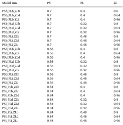
Instead of conducting a rigorous and computationally expensive sensitive analysis, a preliminary and simpler sensitivity analysis was carried out. To see how sensitive the model was to the production of the vertebrate groups, parameters that control recruitment (α in the Beverton-Holt function, Eq. (2), and a parameter controlling the con-stant recruitment per adult) were increased and decreased one at a time by 20%. A sensitivity analysis was also conducted to assess how sen-sitive the model was to production of the low trophic levels groups (phytoplankton and zooplankton) by altering their production by 20% and considering interactions between the selected parameters (Table 3), as was done for the Atlantis model of the Benguela system ( Ortega-Cisneros et al., 2017). How sensitive the model was to the oceano-graphic data (temperature, salinity and waterfluxes) was also explored. It is common to repeat years of oceanographic data in Atlantis models for the hindcast (Nyamweya et al., 2016;Ortega-Cisneros et al., 2017) and forecast (Kaplan et al., 2012). In the present model there are time-series of oceanographic data of 65 years which cover the whole simu-lated period. To explore the effects of oceanographic data,five of the warmest years (2003–2007) were repeated 13 times to cover the 65 year simulation run (Fig. 3) and effects on biomass of the functional groups in the model were assessed.

When only one parameter was perturbed at a time, as was done with the recruitment parameters, a measure of model sensitivity was calcu-lated as described inMurray and Parslow (1997):

= −

S V α V α V α (1.2 ) (0.8 )

0.4 ( ) , ij

i j i j

i j (6)

whereSijis the sensitivity measure for the biomass of groupi when

recruitment parameter (α) in the Beverton-Holt function (see Eq. (2)) is perturbed for groupj,Vi(−)is the average biomass of groupifor the

whole simulated period, i.e.Vi(1.2αj)is the average biomass of groupi

when the recruitment of groupjis increased by 20%. IfS= 1 then the biomass changes by 20% when the recruitment is changed by 20%. If S> 1 then the change in biomass is higher and if S< 1 then the change in biomass is lower.

The measureSis no longer applicable when sensitivity to interac-tions between parameters is explored. Instead percentage change in biomass is used to measure sensitivity. The same was also done when examining the effects of the oceanographic data. In that case, the effects the oceanographic data had on the trend of the biomass was also con-sidered. This was achieved by calculating the correlation of biomass from the base run and biomass under the modified oceanographic run.

3. Results and discussion

3.1. Species interactions

An important part of ecosystem modeling is modeling the species (or functional groups) interactions. This was done using the Holling type II function (Eq. (1)). The diet composition of the predators re-sembled what was observed in the stomach content data for most groups (Figs. 4 and 5). The predators were feeding on the correct groups, but they were relying too much on zooplankton and benthic invertebrates in the model than what the stomach data indicated. The zooplankton could however be under-represented in the stomach con-tent data because of differences in digestion rates (Hyslop, 1980). Bias towards the invertebrates will result in weaker species interactions between the vertebrate groups. Also, sandeel were not as large a com-ponent of the diet of its predators as they should have been. However that group collapsed over time in the model, which it also did in the ecosystem (Lilliendahl et al., 2013).

How much each group needs to feed to maintain their individual weight was modeled with the assimilation parameter (E) in the Holling type II function (Eq. (1)) and with the respiration function (Audzijonyte et al., 2017a). The weight each group loses due to spawning also affects how much they need to consume to maintain their weight. This, along with the diet composition, controls how strong the species interactions are. The Atlantis model does not report detailed consumption statistics and therefore results on this are not shown. The strength of the species interactions can be investigated using a sensitivity analysis as was the case in this study (see Section3.3).

3.2. Simulated biomass and landings

There were few groups with biomass that decreased substantially towards the end of the model run. These groups were: sandeel (6% of initial biomass), gelatinous zooplankton (10% of initial biomass), pico-phytoplankton (10% of initial biomass), macroalgae (7% of initial biomass) and dinoflagellates (0.1% of initial biomass). Sandeel was also observed to decline in the ecosystem (Lilliendahl et al., 2013). The biomass of pico-phytoplankton has very large seasonal variations and is reported for January in the model when it is lowest, but the initial biomass represents the situation during the summer months. The bio-mass of gelatinous zooplankton and macroalgea decreased to 7–10% of its initial biomass, but because they still exist in the system and because they are not important part of the diet of other groups (except benthic grazers) this should not cause problems for the behavior of the system. The dinoflagellates were a group that went close to extinction. The sensitivity study showed that this group is outcompeted by the pico-phytoplankton (see Section3.3.2). The abundance of the other two

Table 3

Growth rate of pico-phytoplankton (PS), diatoms (PL) and macrozooplankton (ZL) in the base run (b) and where these parameters were decreased by 20% (d) or increased by 20% (i).

Model run PS PL ZL

PSb_PLb_ZLb 0.7 0.4 0.8

PSb_PLb_ZLd 0.7 0.4 0.64

PSb_PLb_ZLi 0.7 0.4 0.96

PSb_PLd_ZLb 0.7 0.32 0.8

PSb_PLd_ZLd 0.7 0.32 0.64

PSb_PLd_ZLi 0.7 0.32 0.96

PSb_PLi_ZLb 0.7 0.48 0.8

PSb_PLi_ZLd 0.7 0.48 0.64

PSb_PLi_ZLi 0.7 0.48 0.96

PSd_PLb_ZLb 0.56 0.4 0.8

PSd_PLb_ZLi 0.56 0.4 0.64

PSd_PLb_ZLd 0.56 0.4 0.96

PSd_PLd_ZLb 0.56 0.32 0.8

PSd_PLd_ZLd 0.56 0.32 0.64

PSd_PLd_ZLi 0.56 0.32 0.96

PSd_PLi_ZLb 0.56 0.48 0.8

PSd_PLi_ZLd 0.56 0.48 0.64

PSd_PLi_ZLi 0.56 0.48 0.96

PSi_PLb_ZLb 0.84 0.4 0.8

PSi_PLb_ZLi 0.84 0.4 0.64

PSi_PLb_ZLd 0.84 0.4 0.96

PSi_PLd_ZLb 0.84 0.32 0.8

PSi_PLd_ZLd 0.84 0.32 0.64

PSi_PLd_ZLi 0.84 0.32 0.96

PSi_PLi_ZLb 0.84 0.48 0.8

PSi_PLi_ZLd 0.84 0.48 0.64

phytoplankton groups seems to be sufficient to make the system dy-namics work, but the model would be more stable if it was possible to achieve balance between the phytoplankton groups.

The simulated biomass changes either because individual weight changes (Fig. 6), the numbers changes, or both. The simulated biomass of some of the commercialfish groups (Fig. 7) increased in the start of the model run, but decreased rapidly when fishing pressure was in-creased. The exception was for the blue whiting, which dropped in biomass at the start of the model run, when the individual weight dropped (Fig. 6k), and did not increase until around 1980, but then showed a decreasing trend when harvesting of that group begin around 2000 (Fig. 7k). Mackerel was modeled as an invasive species and its biomass increased rapidly after 2000 (Fig. 7l). The burn in period was included in the model run, which can explain the rapid changes at the start of the simulation when the model has not stabilized.

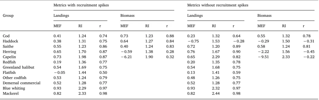
The simulated biomass trajectories offive groups were compared to estimated biomass with and without recruitment spikes (Fig. 7). The skill assessment showed that the simulated biomass of codfitted best to the estimated biomass (Fig. 7a), both MEF and the correlation were the highest and RI the lowest (Table 4). The simulated biomass of the pe-lagic species, herring and capelin (Fig. 7d and e), did notfit the ob-servations as well as the biomass of the demersal species and had a MEF lower than zero and a weak correlation. When the recruitment spikes were taken out of the model, thefit became worse for all thesefive groups. The cod and the saithe had positive MEF and high, positive correlation without the recruitment spikes but haddock, capelin and herring in the model were not able to get the trend in biomass without

having the recruitment spikes included.

The model cannot be expected to achieve the correct trend when forecasting for the groups that required recruitment spikes to achieve positive correlation in the skill assessment. However, it is possible to achieve uncertainty in the forecast by running the model under dif-ferent recruitment processes. It also must be kept in mind that this is an ecosystem model and not intended for tactical advice, but rather for strategic advice where the accuracy of specific annual recruitment es-timates is not as important.

The simulated landings, which were forced in the model with a time-series of harvest rates had reasonablefit to the data for most of the 12 groups (Fig. 8). Saithe (Fig. 8c), other codfish (Fig. 8i) and the de-mersal commercial group (Fig. 8j) had a goodfit in terms of all three metrics (Table 4). The landings of theflatfish group (Fig. 8h) had the poorestfit, with the MEF just above zero and a correlation of 0.58. The MEF was positive for all groups, except for haddock when it was modeled without recruitment spikes (Fig. 8b andTable 4). The mag-nitude of the simulated landings was not far offfor most groups; seven of the groups were within 50% of their observed values. Note that the RI index is very sensitive if there are a few years where the magnitude is incorrect. This was the case for blue whiting and mackerel where the landings were very low is some years. In these cases, the total difference in tons was not high, but because the landings were low, the difference in magnitude could be large. All groups had positive correlation to the landings data except haddock, which had a negative correlation when the model had no recruitment spikes. The correlation decreased for the cod when the recruitment spikes were taken out of the model, but

Fig. 3.Temperature in the 50–150 m layer in box 25 (south of Iceland, seeFig. 1) and in box 37 (north of Iceland, seeFig. 1) from 1948 to 2012 when the full

increased for the saithe. Modeling without the recruitment spikes did not have as much of a negative effect on the landings as it did on the biomass for the pelagic groups (i.e. capelin and herring). It was possible

to get a negative correlation for the biomass but positive correlation for the landings (Table 4).

Skill assessment has now been conducted for most recent Atlantis models, e.g. for Lake Victoria (Nyamweya et al., 2016) and the Ben-guela and Agulhas currents (Ortega-Cisneros et al., 2017). The present model has similar skill as these two models where most groups had correlation higher than 0.5 and positive MEF. Skill assessment has been performed for Atlantis models using biomass estimates ( Ortega-Cisneros et al., 2017) or catch per unit effort where biomass estimates were not available and landings data (Nyamweya et al., 2016).Olsen et al. (2016)also used ecosystem indicators to conduct skill assessment for the Atlantis model for the northeast US. This was not attempted for the present model as the data needed to calculate these indicators were not available.

Discards were simulated for cod and haddock and compared to es-timated discards (Fig. 8). The discard rate was on average 3.8% for cod and 7.0% for haddock over the simulated period when recruitment was modeled with recruitment spikes. This is consistent with what has been estimated for haddock, where the discard rate has been estimated to be from 2 to 22% in the last three decades (Pálsson, 2002;Pálsson et al., 2012). The simulated discard rate for cod was higher than what has been estimated, about 1% in recent years (Pálsson et al., 2012), but no estimates exist from the last century. Note that the method used to estimate the discard rate estimated the minimum rate and that the actual discard rate can be assumed to be higher.

3.3. Sensitivity analysis

3.3.1. Recruitment parameters

For each group, altering the recruitment parameter for the group had an effect on that group, but the size of that effect varied greatly among groups (Fig. 9). The groups which that were the most sensitive to changes in the recruitment parameters were herring, mackerel, sandeel, seabirds and pinnipeds. Redfish, capelin, long lived demersal, small sharks and tooth whales were the least sensitive.

Fig. 4.The average simulated diet composition for the

ver-tebrate groups (age-class 4) over the period 1948–2012. Some of the prey groups have been aggregated into the following groups: demersal (all other demersalfish), pelagic (all pelagic fish except herring and capelin), mammals (all mammals and seabirds), zoo (all zooplankton groups), benthos (all benthic invertebrates) and detritus (detritus and discards).

Fig. 5.Average diet composition from stomach content data that was available

The change in the recruitment parameter was 20%, but the change in actual recruitment could be much greater over time because of the shape of the Beverton-Holt curve. The asymptote of the curve was in-creased, which leads to higher recruitment. With higher recruitment the stock can recover over time and produce higher spawning stock that shifts the population to the right of the curve which will consequently lead to even more recruitment, if the recruitment was not at the max-imum in the base run. This was the case for herring, mackerel and sandeel, which hadS> 1 (Fig. 9). The seabird, large shark and the mammal groups were modeled with constant recruitment per adult with no explicit asymptote. Changing the recruitment parameter for these groups by 20% also led to a greater change in actual recruitment by the end of the model run.

Most of the groups hadS< 1 which means that changing the re-cruitment parameters by 20% resulted in less than a 20% change in the

biomass. This was because other parameters affected how much groups could increase in biomass. The quadratic mortality parameter controls the density dependent non-predation mortality; as numbers in an age-class increase so does the mortality. Cannibalism also restrains popu-lation growth when recruitment is increased and this may be the reason why the stock size for the redfish group changed little with increased recruitment. Also, redfish is a long-lived group (5 years within an age-class), which means that it takes a long time for the change in re-cruitment to have an effect on the numbers in the older age-classes. Changing the maximum recruitment of capelin by 20% had little effect on its biomass (S= 0.11). The capelin numbers increased when max-imum recruitment was increased by 20%, but the individual weight dropped, resulting in very similar biomass as in the base run. The in-verse happened when maximum recruitment was decreased, their numbers decreased but individual weight increased and resulted in

similar biomass.

Saithe, redfish and tooth whales had the largest effect on other vertebrate groups which were mostly negative effect on their prey groups. They also had positive effects on few groups by affecting the biomass of their predators. Vertebrate groups that were the most sen-sitive to changes in the recruitment of other groups were mackerel, flatfish, sandeel, small pelagicfish, seabirds and minke whale. It was necessary to analyze what the effects were on individual weight (re-serve and structural weight) and numbers rather than simply con-sidering their biomass to understand how the groups affected each other. It is also helpful to look at the diet composition of the groups to understand their interactions.

Groups can have an effect on other groups if they feed on that group or if they feed on its predators. For example, redfish had an effect on saithe (S=−0.28) because it feeds on it, even though saithe only

makes up a very small portion of the redfish diet. Redfish had an op-posite effects on theflatfish group (S= 0.35) by consuming the pre-dators offlatfish, such as saithe.

There can also be indirect effects on a group if they compete for the same prey groups. For example, altering the recruitment of sandeel affected theflatfish group (S=−0.33). The individual weight offl at-fish increased when the recruitment of sandeel was decreased and vice versa when the recruitment was increased. That affected the spawning biomass of theflatfish, which consequently affected the recruitment leading to changes in their numbers and biomass.

Altering the recruitment of the vertebrate groups also had an effect on the invertebrates, primary producers and the detritus groups (Fig. 10). The most sensitive groups were pico-phytoplankton and mi-crozooplankton. The seagrass and benthic invertebrate groups were not sensitive to a change in the recruitment of the vertebrates except the

benthic grazer group, which was sensitive towards a change in sandeel and haddock recruitment. Capelin and sandeel seemed to have the most effect on the plankton groups but had opposite effects on the pico-phytoplankton. Both these groups had high biomass (at least at the start of the model run) and have zooplankton as the most important com-ponent of their diet, but sandeel also relies on benthic invertebrates. Dinoflagellates were a group that went close to extinction (0.1% of its initial biomass) throughout the base model run, but altered recruitment of cod and sandeel changed its biomass. The low biomass of the dino-flagellates should not be a problem as the other two phytoplankton groups compensated for the low biomass of them.

It has been observed that removal of top predators can have cas-cading effects down the food web, where the removal led to 45% de-crease in large zooplankton and a slight inde-crease in phytoplankton (Frank et al., 2005). The changes in recruitment of vertebrate groups led to large changes in phytoplankton biomass that may not be realistic and this should be studied further before the model is used for man-agement strategy evaluation.

3.3.2. Growth parameters of plankton groups

The effects of changing the growth parameters of pico-phyto-plankton, diatoms and macrozooplankton on the biomass of the func-tional groups in the model are given inFig. 11. Changing the growth rate of the macrozooplankton had very little effect except when the growth rate of diatoms had also been increased. The results of altering the growth rate of the macrozooplankton are therefore not discussed further here. Dinoflagellates appeared to suffer competitive exclusion, being outcompeted by the pico-phytoplankton (for example, dino-flagellates multiply when the growth rate of the pico-phytoplankton is decreased;Fig. 11). This increased biomass of dinoflagellates led to an increased biomass of microzooplankton.

The change in the growth of the phytoplankton also had a con-siderable effect on the vertebrate groups. The vertebrate groups that were the most sensitive were: baleen whales, minke whale, seabirds, small and large pelagicfish, sandeel, mackerel and blue whiting, ca-pelin and redfish (Fig. 11). Zooplankton is a large portion of the diet of these groups (Fig. 4) and as the zooplankton responded to the phyto-plankton, these planktivorous feeders did as well. The redfish biomass increased by 84% when the growth rate of pico-phytoplankton was decreased and the rate of diatoms was increased. All vertebrate groups increased in biomass when the growth rate of both the phytoplankton groups was increased and all vertebrate groups except mackerel de-creased in biomass when just the diatom growth rate was reduced (Fig. 11). A sensitivity study on the Atlantis model for the Benguela system also showed strong reactions to changes in the growth rate of the plankton groups, where some of thefish groups showed more than

100% increase in biomass (Ortega-Cisneros et al., 2017).

3.3.3. Oceanographic data

Repeating thefive warm years instead of having the full oceano-graphic time series affected some of the functional groups. Temperature affects the respiration of the vertebrate groups and consequently their growth. The waterfluxes were also different between the two model runs, influencing advection of nutrients and plankton groups; the shift in nutrients also affected the growth of the primary producers. This methodology can be used when testing the effect of climate change that could have larger effects on the groups, especially the vertebrate groups if density-dependent movement is turned on in the model, which was not the case in the present model.

The oceanographic data had a large effect on the biomass of the phytoplankton groups: pico-phytoplankton and diatoms (Fig. 12a). The biomass of the pico-phytoplankton increased, while the biomass of the diatoms decreased. Diatoms need higher nutrient concentrations than pico-phytoplankton to achieve their maximum growth rates. The warm conditions and associated waterfluxes were therefore more favorable for the pico-phytoplankton. The warm conditions were also favorable for cephalopods, capelin and mackerel, leading to increased biomasses compared to the base run. In contrast, these conditions led to decreased biomass of herring. Capelin and herring feed mostly on zooplankton, but capelin feeds both on mesozooplankton and macrozooplankton, while herring feeds mainly on macrozooplankton, which increased in biomass while the mesozooplankton decreased in biomass. It was ne-cessary to look at the output from the model for each spatial box to better understand why the capelin biomass was higher in the case when thefive warm years were repeated. At the individual spatial box level, it was observed that the biomasses of both mesozooplankton and mac-rozooplankton were much higher in one box in the north, where the capelin feed during the winter (Box 12, Fig. 1), with the modified oceanography than in the base run. The model output had to be ex-plored at a high temporal resolution to better understand why the herring biomass was lower when the warm years were repeated. The reserve to structural weight ratio of the herring is lower in the early years of the simulation with modified oceanography, which affected the recruitment and ultimately led to a lower number of adults later in the simulation (perpetuating lower recruitment).

Using thefive warm years did not have a substantial effect on the trend of the biomass of the vertebrate groups (Fig. 12b), not even herring and capelin, which had changes in total biomass. It did have some effect on the large pelagic fish, baleen whales and the other toothed whales. The correlation between the zooplankton and phyto-plankton groups was low, indicating that the trend was different from the base run. The other benthic filter feeders group had a negative

Table 4

Skill assessment with and without recruitment spikes: The three metrics model efficiency (MEF), reliability index (RI) and correlation (r) for biomass and landings (see Eqs. (3)−(5) for the metrics).

Metrics with recruitment spikes Metrics without recruitment spikes

Group Landings Biomass Landings Biomass

MEF RI r MEF RI r MEF RI r MEF RI r

Cod 0.41 1.24 0.74 0.73 1.23 0.88 0.23 1.32 0.64 0.55 1.32 0.78

Haddock 0.38 1.31 0.75 0.64 1.27 0.84 −0.75 1.53 −0.28 −0.29 1.50 −0.31

Saithe 0.55 1.23 0.86 0.40 1.24 0.83 0.72 1.20 0.89 0.58 1.24 0.81

Herring 0.65 1.70 0.87 −0.59 1.38 0.28 0.76 1.67 0.90 −2.22 1.56 −0.45

Capelin 0.73 1.98 0.87 −6.21 1.90 0.32 0.65 2.29 0.82 −9.51 2.33 −0.22

Redfish 0.19 1.36 0.77 0.20 1.35 0.78

Greenland halibut 0.54 1.69 0.75 0.54 1.68 0.75

Flatfish −0.05 1.44 0.50 0.13 1.41 0.59

Other codfish 0.53 1.24 0.79 0.48 1.26 0.75

Demersal commercial 0.52 1.28 0.77 0.52 1.28 0.77

Blue whiting 0.93 2.29 0.97 0.93 2.32 0.97

correlation, which means that the trend of the biomass under the modified oceanography was in the opposite direction compared to its biomass in the base run. It is therefore important to have correct oceanographic data if trends of low tropic levels are the focus of a study.

3.4. Model reliability

Kaplan and Marshall (2016)have set some standards that end-to-end models such as Atlantis should reach before they are used in management strategy evaluations. Models should fulfill the following:

1) All biological functional groups should persist throughout the model run.

2) The model should achieve equilibrium, i.e., under fixed

environmental forcing the unfished model should have stable bio-mass over thefinal 20 years for most vertebrate groups.

3) The biomass trends should be compared to survey time-series (hindcast).

4) Qualitative model comparisons to survey data.

5) The model should capture the dynamics of abundant species. 6) Most functional groups should qualitatively match expected

pro-ductivity.

7) Natural mortality should be realistic.

8) Age and length structure of vertebrate groups should match data. 9) Diet composition of the functional groups should match diet data.

In relation to these standards, all groups except the dinoflagellates (which had only 0.1% of its initial biomass) persisted throughout the model run. Few groups (sandeel, gelatinous zooplankton,

phytoplankton and macroalgae) decreased considerably in biomass but still persisted at the end of the model when they had 7–10% of its initial biomass.

Kaplan and Marshall (2016)did not define what is considered stable biomass. In this study stable biomass will be considered if the biomass changes by less than 10% over the last 20 years of the simulated period. The model was run 100 years further, with the samefishing pressure that was used in the final year of the base model and with

oceanography rerunning from the start of the model run. After 100 years of forecast 23 of the 26 vertebrate and 14 of the 16 invertebrate groups had stable biomass in the last 20 years of the model run. If fishing was excluded from the model and the model run was 165 years only 15 of the 26 vertebrate groups had stable biomass in the last 20 years of the model run. Herring showedfluctuations and did not have any trend if more than 20 years were considered. It is not realistic here for all groups to reach a perfectly constant biomass as the underlying

Fig. 9.Sensitivity analysis: the metric S (see Eq. (6)) for the change in biomass of the vertebrate groups when recruitment was altered for the vertebrate groups. The

grey color represent S <−1 or S > 1.

Fig. 10.Sensitivity analysis: the metric S (see Eq. (6)) for the change in biomass of the invertebrate, primary producer, bacteria and detritus groups when recruitment

physical model always has some fluctuations. The physical forcing (oceanographic data) contains seasonal and annual variations in tem-perature, salinity and waterfluxes, which consequently leads to fluc-tuations in phytoplankton biomass, which escalates up the food chain. It is difficult to assess what groups compose the same trend as the phytoplankton because of the large variation in phytoplankton biomass, both in space and time.

Most of thefish groups had realistic natural mortality that decreased with age. Capelin had higher mortality for adults than juveniles, but that group is set as semelparous, i.e., allfish die after spawning. The whale groups had lower mortality for the juveniles. This is a con-sequence of the quadratic mortality parameter settings used for this group (which is different between juveniles and adults). This should be fixed by increasing the mortality for the juveniles and the recruitment rate in order to maintain suitable biomass levels and trajectories before

the model is used to predict effects on the whale groups or scenarios regarding whaling.

The model was calibrated so that the weight (or length) of each age-class within a group would be relatively constant over time (< 20% change from initial conditions). This was achieved for most groups, but some age-classes went over (or under) the limit (Fig. 6).

The diet composition matched the data (Section3.1). It is a chal-lenging task to calibrate an ecosystem model of this complexity such that both diet composition and changes in diet over time are re-presented correctly. The most important is to get the proportions si-milar in order for the species interactions to be realistic and that has been accomplished for the current model. Minor adjustments to the availability of prey or to spatial distribution of the functional groups may improve the model and that can be determined by conducting another skill assessment of an adjusted model.

The simulated biomass was compared to biomass estimates and si-mulated landings to landings data and a skill assessment conducted (Section3.2).Kaplan and Marshall (2016)did not state how well the model needs tofit to the data before it is considered reliable and neither didOlsen et al. (2016). However, it can be concluded that models that cannot replicate historical time-series will not be able to produce reli-able predictions about the future. Modeled groups that have negative correlation in the skill assessment do not replicate historical time-series. It is more difficult to define what values the metrics MEF and RI need to reach to be able to conclude that the model is reliable. When MEF < 0 then a straight line through the average would give a betterfit, but if the correlation is positive the model can still be useful and the same can be said about high RI. The model could however be used with more confidence when the correlation, MEF and RI are close to 1 but the minimum requirement is that the correlation is positive. The skill as-sessment showed that the model had a good fit to the data, when modeled with recruitment spikes, for the most important commercial groups, i.e. the correlation was positive, MEF > 0 and RI < 1.5 for most groups (Table 4). However, most of the groups in the model had no biomass estimates and are not targeted by thefisheries and therefore had no landings data for calibration and skill assessment purposes. It was therefore not possible to determine the skill of the model for those groups. Some of the non-commercial groups are caught in the survey and it is possible to calculate a survey index for those groups and cal-culate correlation between the simulated biomass and the survey index. However, such analysis was not conducted for this paper because these indices may not be reliable as the survey is not designed to capture population trends for these species. Skill assessment could also be carried out for plankton groups. However, this is challenging as these groups show large variation, both is space and time. It would also be of interest to assess how well the model captures the ocean currents. It can then be evaluated if the model would benefit from an improvement of the spatial structure of the model. This is a work for further research.

Ideally, one should not use the same data for model calibration and for skill assessment of that model (Bennett et al., 2013). This was not possible in this case as all available data were needed for calibration and therefore the model reliability could be overestimated.

3.5. How can this model be used for ecosystem basedfisheries management?

The goals of the Icelandicfisheries management act have largely be met. Since its inception, harvest rates of commercially exploitedfish stocks have gradually been decreased, with the aim of achieving single species maximum sustainable yield. The need for alternative manage-ment strategies that take ecosystem and socio-economic considerations into account has, however, increased in recent years. The model could be used to evaluatefisheries scenarios for the most important com-mercial species taking interactions into account. It provides a solid basis for the testing of alternative ecosystem andfisheries management sce-narios and will be of further use when the socio-ecological model component has been integrated with the biophysical and fisheries

Fig. 11.Sensitivity analysis: Percentage change in biomass of all functional

model components.

This model can be used for examining scenarios regarding discards and by-catch. It has already been used to explore the economic and ecological effects of discarding in the cod and haddockfisheries where five scenarios with different selectivity and discard rates where com-pared (Sturludottir, 2018). The small scale lumpsuckerfishery, which is an important part of a local economy, has been under scrutiny for considerable by-catch of marine mammals and seabirds (Anon., 2018; Pálsson et al., 2015) and the model could be used to evaluate trade-offs of alternative management actions, such as area closures and/or effort reduction, which could have substantial consequences for the coastal communities.

The spatial component of the Atlantis model allows diverse sce-narios to be explored. For example the effects of changes in spatial movement of species because of climate change can be explored, but such changes have already been observed in Icelandic waters (Carscadden et al., 2013). The effects of seasonal or permanent closures already implemented in Icelandic waters have been studied (Schopka, 2007;Woods et al., 2017), but the effects of potential closures could be explored with the current model.

The model is being used as an operating model to evaluate the

performance of other simpler ecosystem models such as EwE and Gadget. It is very difficult to evaluate the reliability of ecosystem models, but skill assessment has been used in that purpose. Atlantis models can be used to test if other models can imitate the“Atlantis ecosystem”. Data are simulated from the known ecosystem and im-ported into the other models and then compared to the true values from the Atlantis model. Using this method it can be studied how well the models need tofit to historical data to be deemed reliable when used for forecasting. This work is now ongoing using the present model.

4. Conclusion

An end-to-end model has been constructed that resembles the eco-system of the Icelandic waters. This is the first dynamic end-to-end model for this area. Preliminary EwE models (Buchary, 2001;Mendy, 1998) and multi-species models (Elvarsson, 2015) have been con-structed but no dynamic models where the entire ecosystem is simu-lated. Fisheries management in Iceland aims to be ecosystem based and this model can be used to support EBFM. It can be used to evaluate differentfisheries and climate scenarios and to conduct management strategy evaluations. The focus of the model is on the most important

Fig. 12.The effects of the oceanographic data, whenfive years of oceanographic data were repeated from 1948 to 2012 a) Change in biomass from the base run

commercial groups, to explore the effects of various harvesting strate-gies, such as area closures and selectivity changes, on both commercial groups and on other parts of the ecosystem. The model needs to be judged to be reliable to have confidence in the model as a basis for assessments and projections. It is very difficult to estimate the relia-bility of a model as complex as Atlantis. Nevertheless, it was possible to carry out a skill assessment, which showed that the model was able to simulate the biomass trends for the most important commercial groups. There were limited data available on the non-commercial groups and therefore the reliability of the model for those groups could not be assessed. Therefore, predicted effects on those groups need to be taken with caution.

The sensitivity analysis revealed the influence of key parameters and inputs, e.g., recruitment parameters and oceanographic data, on model projections. This showed that there was uncertainty due to sensitivity to the form of the recruitment relationships used and due to the effect of environmental conditions (something the model may not capture well). Uncertainty also exists due to sensitivity of the model to oceanographic forcing, meaning that care must be taken around as-sumptions regarding prevailing oceanographic conditions used when running simulations, such as warm vs. cold periods.

Ecosystem models such as Atlantis are in a constant process of further improvement and this is the case with the current model. This work, the skill assessment and the sensitivity study will facilitate that process by increasing the understanding of the dynamics of the system.

Acknowledgments

This study has received funding from the European Union’s Seventh Framework Programme for research, technological development and demonstration under grant agreement no. 613571 for the project MareFrame and from the European Commission’s Horizon 2020 Research and Innovation Programme under Grant Agreement No. 634495 for the project Science, Technology, and Society Initiative to minimize Unwanted Catches in European Fisheries (Minouw). Funding from the Icelandic Research Fund (rannis, No. 152039051) is also ac-knowledged. We would like to thank Sólveig Rósa Ólafsdóttir, Guðmundur Þórðarson, Gísli A. Víkingsson, Þorvaldur Gunnlaugsson, Kristján Lilliendahl, Ástþór Gíslason, Héðinn Valdimarsson and Jónas Páll Jónasson at the Marine and Freshwater Research Institute and Guðmundur Guðmundsson at the Icelandic Institute of Natural History for their contribution to this work. We would also like to thank two anonymous reviewers for their valuable comments.

References

Anon, 2010. Manuals for the Icelandic Bottom Trawl Surveys in Spring and Autumn. Hafrannsoknir nr. 156. The Marine Research Institution, Reykjavik, Iceland. https:// www.hafogvatn.is/static/research/files/fjolrit-156pdf.

Anon, 2015. Environmental Conditions in Icelandic Waters 2014. Hafrannsoknir nr. 181. The Marine Research Institution, Reykjavik, Iceland. https://www.hafogvatn.is/ static/research/files/fjolrit-181pdf.

Anon, 2016. State of Marine Stocks in Icelandic Waters 2015/2016 and Prospects for the Quota Year 2016/2017. Marine Research in Iceland 185. The Marine Research Institution, Reykjavik, Iceland. https://www.hafogvatn.is/static/research/files/ fjolrit_185pdf.

Anon, 2018. Bycatch of Seabirds and Marine Mammals in Lumpsucker Gillnets 2014-2017. The Marine and Freshwater Research Institution, Reykjavik, Iceland. https:// www.hafogvatn.is/static/files/skjol/techreport-bycatch-of-birds-and-marine-mammals-lumpsucker-en-final-draft.pdf.

Astthorsson, O.S., Gislason, A., Jonsson, S., 2007. Climate variability and the Icelandic marine ecosystem. Deep-Sea Res. II 54, 2456–2477.

Audzijonyte, A., Gorton, R., Kaplan, I., Fulton, E.A., 2017a. Atlantis User’s Guide Part I: General Overview, Physics & Ecology. CSIRO, Hobart, Australia.

Audzijonyte, A., Gorton, R., Kaplan, I., Fulton, E.A., 2017b. Atlantis User’s Guide Part II: Socio-Economics. CSIRO, Hobart, Australia.

Bennett, N.D., Croke, B.F., Guariso, G., Guillaume, J.H., Hamilton, S.H., Jakeman, A.J., Marsili-Libelli, S., Newham, L.T., Norton, J.P., Perrin, C., Pierce, S.A., 2013. Characterising performance of environmental models. Environ. Model. Softw. 40, 1–20.

Buchary, E.A., 2001. Preliminary reconstruction of the Icelandic marine ecosystem in

1950 and some predictions with time series data. Fisheries Impacts of the North Atlantic Ecosystems: Models and Analyses. Fisheries Centre Research Reports, vol. 9. pp. 296–306 (4).

Carscadden, J.E., Gjøsæter, H., Vilhjálmsson, H., 2013. A comparison of recent changes in distribution of capelin (Mallotus villosus) in the Barents Sea, around Iceland and in the Northwest Atlantic. Prog. Oceanogr. 114, 64–83.

Christensen, V., Walters, C.J., 2004. Ecopath with Ecosim: methods, capabilities and limitations. Ecol. Model. 172 (2–4), 109–139.

Csardi, G., Nepusz, T., 2006. The igraph software package for complex network research. InterJournal, Complex. Systems 1695. http://igraph.org.

Elvarsson, B., 2015. Statistical Models of Marine Multispecies Ecosystems. PhD Thesis. University of Iceland, Reykjavik, Iceland.

Forrest, R.E., Savina, M., Fulton, E.A., Pitcher, T.J., 2015. Do marine ecosystem models give consistent policy evaluations? A comparison of Atlantis and Ecosim. Fish. Res. 167, 293–312.

Frank, K.T., Petrie, B., Choi, J.S., Leggett, W.C., 2005. Trophic cascades in a formerly cod-dominated ecosystem. Science 308 (5728), 1621–1623.

Fulton, E.A., 2010. Approaches to end-to-end ecosystem models. J. Mar. Syst. 81 (1), 171–183.

Fulton, E.A., Smith, A.D.M., Smith, D.C., 2007. Alternative Management Strategies for Southeast Australian Commonwealth Fisheries: Stage 2: Quantitative Management Strategy Evaluation. CSIRO, Tasmania, Australia.https://research.csiro.au/atlantis/ wp-content/uploads/sites/52/2015/10/AMS_Final_Report_v6.pdf.

Fulton, E.A., Link, J.S., Kaplan, I.C., Savina-Rolland, M., Johnson, P., Ainsworth, C., Horne, P., Gorton, R., Gamble, R., Smith, A.D.M., Smith, D.C., 2011. Lessons in modelling and management of marine ecosystems: the Atlantis experience. Fish Fish. 12 (2), 171–188.

Gislason, A., Valdimarsson, H., Guðmundsson, K., Olafsdottir, S.R., 2016. Environmental Conditions in Icelandic Waters 2015. [In Icelandic with English summary]. Marine and Freshwater Research Institution, Reykjavik, Iceland.https://www.hafogvatn.is/ static/research/files/hafogvatn2016-001_lokapdf.

Gunnarsson, K., Jónsson, G., Pálsson, O.K., 1998. Sjávarnytjar við Ísland (e. Marine Resources around Iceland). Mál og Menning, Reykjavik, Iceland [in Icelandic]. Hilborn, R., 2007. Defining success infisheries and conflicts in objectives. Mar. Policy 31

(2), 153–158.

Hudson, L., Reuman, D., Emerson, R., 2016. Cheddar: Analysis and Visualisation of Ecological Communities. R Package Version 0.1-631.

Hyslop, E.J., 1980. Stomach contents analysis–a review of methods and their application. J. Fish Biol. 17, 411–429.

Jónsson, G., Pálsson, J., 2013. Íslenskirfiskar (e. Icelandic Fish). Mál og menning, Reykjavík, Iceland [In Icelandic].

Kaplan, I.C., Marshall, K.N., 2016. A guinea pig’s tale: learning to review end-to-end marine ecosystem models for management applications. ICES J. Mar. Sci. 73 (7), 1715–1724.

Kaplan, I.C., Horne, P.J., Levin, P.S., 2012. Screening California currentfishery man-agement scenarios using the Atlantis end-to-end ecosystem model. Prog. Oceanogr. 102, 5–18.

Kaplan, I.C., Holland, D.S., Fulton, E.A., 2014. Finding the accelerator and brake in an individual quotafishery: linking ecology, economics, andfleet dynamics of US West Coast trawlfisheries. ICES J. Mar. Sci. 71 (2), 308–319.

Lilliendahl, K., Solmundsson, J., 1997. An estimate of summer food consumption of six seabird species in Iceland. ICES J. Mar. Sci. 54, 624–630.

Lilliendahl, K., Hansen, E.S., Bogason, V., Sigursteinsson, M., Magnúsdóttir, M.L., Jónsson, P.M., Helgason, H.H., Óskarsson, G.J., Óskarsson, P.F., Sigurðsson, Ó.J., 2013. Viðkonubrestur lunda og sandsílis við Vestmannaeyjar (e. Recruitment failure of Atlantic puffins Fratercula arctica and saneels Ammodytes marinus in Vestmannaeyjar islands). Náttúrufræðingurinn 83 (1–2), 65–79 [in Icelandic with English summary].

Link, J.S., 2002. What does ecosystem-basedfisheries management mean. Fisheries 27 (4), 18–21.

Logemann, K., Ólafsson, J., Snorrason, Á., Valdimarsson, H., Marteinsdóttir, G., 2013. The circulation of Icelandic waters–a modelling study. Ocean Sci. 9 (5), 931–955. Matthíasson, T., 2003. Closing the open sea: development offishery management in four

Icelandicfisheries. Nat. Resour. Forum 27 (1), 1–18 Blackwell Publishing Ltd. Mendy, A., 1998. Trophic Modeling as a Tool to Evaluate and Manage Iceland’s

Multispecies Fisheries. Final project, United Nations University–Fisheries Training Programme, Reykjavik, Iceland.

Murray, A., Parslow, J., 1997. Port Phillip Bay Environmental Study: Final Report. CSIRO, Canberra, Australia. https://publications.csiro.au/rpr/download?pid=

procite:1e941c7a-3303-4b90-ba69-ecad2a810020&dsid=DS1.

Nyamweya, C., Sturludottir, E., Tomasson, T., Fulton, E.A., Taabu-Munyaho, A., Njiru, M., Stefansson, G., 2016. Exploring Lake Victoria ecosystem functioning using the Atlantis modeling framework. Environ. Model. Softw. 86, 158–167.

Oakley, J.E., O’Hagan, A., 2004. Probabilistic sensitivity analysis of complex models: a Bayesian approach. J. R. Stat. Soc.: Ser. B Stat. Methodol. 66 (3), 751–769. Olsen, E., Fay, G., Gaichas, S., Gamble, R., Lucey, S., Link, J.S., 2016. Ecosystem model

skill assessment. Yes we can!. PLoS One 11 (1), e0146467.

Ortega-Cisneros, K., Cochrane, K., Fulton, E.A., 2017. An Atlantis model of the southern Benguela upwelling system: validation, sensitivity analysis and insights into eco-system functioning. Ecol. Model. 355, 49–63.

Pálsson, Ó.K., 2002. Brottkast ýsu á Íslandsmiðum (e. Discards of haddock in Icelandic waters). Ægir 95, 32–37 [in Icelandic].

Pálsson, Ó.K., Gunnlaugsson, P., Ólafsdóttir, D., 2015. By-Catch of Sea Birds and Marine Mammals in Icelandic Fisheries. Hafrannsóknir nr. 178. [In Icelandic with English summary]. The Marine Research Institution, Reykjavík, Iceland. https://www. hafogvatn.is/static/research/files/fjolrit-178pdf.

Pantus, F.J., 2007. Sensitivity Analysis for Complex Ecosystem Models. PhD Thesis. School of Physical Sciences, the University of Queensland, Australia. http://www. espace.library.uq.edu.au/view/UQ:137017.

Plagányi, É.E., 2007. Models for an Ecosystem Approach to Fisheries (No. 477). Food and Agriculture and Organization of the United Nations, Rome, Italy.

Pope, J., Bartolino, V., Bauer, B., Horbowy, J., Ribeiro, J., Sturludottir, E., Thorpe, R., 2018. Comparing steady state results of a range of multispecies models between and across geographical areas by the use of the Jacobian matrix of yield onfishing mortality rate. Fish. Res.

Saltelli, A., Ratto, M., Tarantola, S., Campolongo, F., 2006. Sensitivity analysis practices: strategies for model-based inference. Reliab. Eng. Syst. Saf. 91 (10), 1109–1125. Saltelli, A., Annoni, P., Azzini, I., Campolongo, F., Ratto, M., Tarantola, S., 2010. Variance

based sensitivity analysis of model output. Design and estimator for the total sensi-tivity index. Comput. Phys. Commun. 181 (2), 259–270.

Schopka, S.A., 2007. Area Closures in Icelandic Waters and the Real-Time Closure System: A Historical Review. Report Series nr.133. [in Icelandic with English summary]. The Marine Research Institution, Reykjavik, Iceland. https://www.hafogvatn.is/static/ research/files/fjolrit-133pdf.

Sigurjonsson, J., Vikingsson, G.A., 1997. Seasonal abundance of and estimated food consumption by cetaceans in Icelandic and adjacent waters. J. Northw. Atl. Fish. Sci. 22, 271–287.

Statistics Iceland, 2017. Retrieved 18th of May 2017 athttp://www.statice.is/. Stefánsson, G., Palsson, O.K., 1997. BORMICON: A Boreal Migration and Consumption

Model. The Marine Research Institution, Reykjavik, Iceland. https://www. hafogvatn.is/static/research/files/fjolrit-058pdf.

Stow, C.A., Jolliff, J., McGillicuddy, D.J., Doney, S.C., Allen, J.I., Friedrichs, M.A., Rose, K.A., Wallhead, P., 2009. Skill assessment for coupled biological/physical models of marine systems. J. Mar. Syst. 76 (1), 4–15.

Sturludottir, E., 2018. Exploring the effects of discarding using the Atlantis ecosystem model for Icelandic waters. Sci. Mar. (Barc.).

Taylor, L., 2005. Definition of areas in Icelandic waters. In: Stefansson, G. (Ed.), Development of Structurally Detailed Statistically Testable Models of Marine Populations. The Marine Research Institution, Reykjavik, Iceland. https://www. hafogvatn.is/static/research/files/fjolrit-119pdf.

Vilhjálmsson, H., 1994. The Icelandic Capelin Stock: Capelin, Mallotus villosus (Muller) in the Iceland–Greenland–Jan Mayen Area. The Marine Research Institution, Reykjavik, Iceland iii_fyrri_hluti_1994pdf, https://www.hafogvatn.is/static/research/files/rit_fiski_x-iii_seinni_hluti_1994pdf.

Vilhjálmsson, H., Carscadden, J.E., 2002. Assessment surveys for capelin in the Iceland–East Greenland–Jan Mayen area, 1978–2001. ICES J. Mar. Sci. 59 (5), 1096–1104.