Modeling the furrow irrigation infiltration function from a single advance point
1
2
3
4
5
6
7
8
9
10
11
12
13
14
15
16
17
18
19 20
21
22
23
24
25
Smith, R.J., Raine, S.R., Langat, P.K., Khatri, K.L.
National Centre for Engineering in Agriculture and Cooperative Research Centre for
Irrigation Futures, University of Southern Queensland, Toowoomba, Queensland, 4350,
Australia
Abstract
Management and control of surface irrigation, in particular furrow irrigation, is limited by
spatio-temporal soil infiltration variability as well as the high cost and time for collecting
intensive field data for estimation of the infiltration characteristics. Recent work has
proposed scaling the commonly used infiltration function using model infiltration curve and a
single advance point for every other furrow in an irrigation event. Scaling factors were
calculated for a series of furrows at two sites at four points down the length of the field
(0.25L, 0.5L, 0.75L and L). Differences in the value of the scaling factor with distance were seen to be a function of the shape of the advance curves. Scaling factor was seen to be
strongly correlated with the furrow wetted perimeter.
Key words: Evaluation, infiltration function, single advance point, furrow irrigation
Introduction
Surface irrigation, specifically furrow irrigation, is the most widely used method of irrigation
in the world despite its low irrigation efficiency attributed mainly to the complexity of the
interactions between field design, soil infiltration characteristics and irrigation management
practice. Irrigation advance data (solution of the inverse problem) is the preferred method to
obtain the infiltration characteristic (most often in the form of the Kostiakov-Lewis equation).
1
2
3
4
5
6
7
8
9
10
11
12
13
14
15
16
17
18
19
20
21
22
23
24
25
this denies the temporal and spatial infiltration variability, which has a significant impact on
irrigation performance (Raine et al. 1997; Mailhol et al. 2005). Temporal infiltration
variability may be managed by real time control, that is, in-field data collection, analysis and
processing during the irrigation (Camacho et al. 1997). Spatial variability requires that a field
representative infiltration function is modified to reflect the variations in hydraulic factors
(for example, wetted perimeter and inflow) and soil intake characteristics across the field
(Clemmens 2000; Strelkoff et al. 2000; Oyonarte et al. 2002).
Past research has attempted to adjust the infiltration function for different inflow rates
(Sepaskhah and Afshar-Chamanabad 2002) or by taking account of wetted perimeter
(Strelkoff and Souza 1984). Camacho et al. (1997) applied volume-balance and kinematic
models (the IPE model) to compute the spatial and temporal variability in real time. The
limitation here has been the quantity of advance data required to characterize the infiltration
equations and the time it takes to process the data. In-field management and control during
irrigation requires quality estimates of infiltration characteristics sufficiently early to allow
timely irrigation decisions to be made. Deriving this infiltration information from minimum
data is important in reducing cost and effort (Gillies and Smith 2005) but comes at the risk of
increased chance of measurement errors.
Recent research has proposed promising methods of reducing the intensive field data
collection required for estimation of the infiltration characteristics and yet still capturing the
soil infiltration variability. Rasoulzadeh and Sepaskhah (2003) used dimensional analysis to
scale infiltration equation for furrow irrigation. They used wetted perimeter to find a
1
2
3
4
5
6
7
8
9
10
11
12
13
14
15
16
17
18
19
20
21
22
23
24
25
this is a complex adjustment of the infiltration function that most irrigators may find difficult
to apply in real time management where data is collected, studied and processed in the field.
The estimation of infiltration parameters using a single advance point and a model infiltration
function is a relatively new concept proposed by Khatri and Smith (2006). They formulated a
scaling factor to be applied in conjunction with the Kostiakov-Lewis infiltration equation to
scale individual infiltration curves within a field. This method is easy to use and operate in
the field as it requires only one advance point measurement along the furrow, plus the inflow
rate and the cross-sectional area of flow at the furrow inlet. Thus, it offers farmers and
advisors considerable savings in the cost and time of field data collection. However, the
method as proposed and tested by Khatri and Smith (2006) arbitrarily used a single advance
point located at 50% of the furrow length (0.5L). This point may be appropriate for long furrows or where long irrigation times are used, but for short furrows requiring short
irrigation durations it may be necessary to measure the advance earlier to allow enough time
for irrigation decisions to be made during the irrigation. However, there is uncertainty over
the effect of the distance at which the advance is measured or the accuracy of the predicted
infiltration and subsequent irrigation modelling.
In this paper the work of Khatri and Smith (2006) is taken further by evaluating the affect
that the location of the single measured advance point along the furrow has on the estimation
of the infiltration. This is of potential importance for in-field irrigation management and
control during irrigation particularly where short field lengths are involved. The ability of the
scaling process to deal with spatial variability in infiltration, including that resulting from
differences in the hydraulic variables such as inflow rate, slope, and wetted perimeter is also
1
2
3
4
5
6
7
8
9
10
MATERIALS AND METHOD
Model infiltration function description
The scaling process proposed by Khatri and Smith (2006) is designed to reduce the amount of
data required to predict the infiltration characteristics for each furrow and for each irrigation
event for a whole field, for the purpose of real-time irrigation management and control. It
involves arbitrary selection of a furrow as a model. Extensive advance and run-off data from
this furrow is used to determine as accurately as possible its infiltration characteristic as
described by the Kostiakov-Lewis equation:
τ
τ o
a f
k
Z = + (1)
where Z is the cumulative infiltration (m3/m), a, k and fo are fitted parameters and τ is the infiltration time (min).
11
12
13
14
15
16
17
18
The cumulative infiltration curve for this furrow becomes the model infiltration function
whose infiltration parameters are then used to estimate (by scaling) cumulative infiltration
functions, for the whole field or other irrigation events, using only one advance point for each
of the remaining furrows or for each subsequent irrigation event. In this scaling process a
scaling factor F is formulated for each furrow or event from volume balance model as:
r tx f x kt
x A t Q F
o a z
o y o
+ + − =
1
σ
σ
(2) 19
20
21
22
23
24
r
pt
x= (3)
1
2 and σzis the sub-surface shape factor for the model infiltration function and calculated as:
) 1 )( 1 (
1 ) 1 (
r a
a r a
z + +
+ − + =
σ (4)
3
4
5
6
7
8
9
The scaling factor F was defined by Khatri and Smith (2006) as the ratio between the infiltrated volume as calculated by the volume balance in the trial furrow at a particular
advance time and the infiltrated volume as calculated by the parameters of the model furrow.
It is applied in conjunction with equation 1 to produce scaled infiltration curves for each
furrow as follows:
{
( ) 0( )}
arg F k τ f τ
Z a
et
t = + (5)
10
11
12
13
14
15
16
17
18
19
20
21
22
23
24
where Ztarget is the cumulative infiltration (m3/m) for the target furrow.
Field data
The data considered in this study were from published field evaluations in two cotton
growing areas, the Bura Irrigation Scheme in Kenya and the Darling Downs in Queensland,
Australia.
Bura Scheme data
Furrow irrigation advance data were collected from the Bura Irrigation Scheme Settlement
Project in Kenya by Mwatha and Gichuki (2000). The soils of the project area are sandy clay
loams and cracking clays with shallowly overlying (about 20 cm) a saline and alkaline
subsoil of low permeability. The evaluation data were collected from four fields of the same
soil and average slopes of 0.09%, 0.13%, 0.25% and 0.31%, denoted in this paper as 9S, 13S,
3.0 ls-1. Furrow spacing was 0.9 m. Parshall flumes placed at 50 m intervals were used to
measure inflow and out flow for each 50 m furrow section. Data only for the fifth irrigation
were used in this study. 1
2
3
4
5
6
7
8
9
10
11
12
13
14
15
16
17
18
19
20
21
22
23
24
25
The data published included furrow characteristics (Table 1), furrow inflow rates and
irrigation advance parameters for two irrigation events in each of the four fields. The
advance parameters for the power advance curve (Table 2) were calculated by Mwatha and
Gichuki (2000) from the measured advance data.
Insert Tables 1 & 2 about here
Australian cotton field data
These data, taken from Khatri and Smith (2006), are from four furrow irrigation events from
a single field (field C) in the Darling Downs region of Southern Queensland, Australia. All
irrigations were conducted by the farm staff using their usual practices. Data collected for
each event included:
• furrow inflow,
• the irrigation advance ( advance times for various points along the furrow including
the time for the advance to reach the end of the furrow), and
• the physical characteristics of the furrow (length, slope and cross-sectional area of
flow).
The flow rate and irrigation advance were measured using the IRRIMATETM suite of tools
developed be NCEA, as described by Dalton et al. (2001). The data are summarized in Table
1
2
3
4
5
6
7
8
9
10
11
12
13
14
15
16
17
18
19
20
21
22
Calculation of infiltration parameters
Infiltration parameters from advance data were obtained for each furrow/event using the
INFILTv5 program (McClymont and Smith 1996). INFILTv5 is a computer software
package for determination of the Kostiakov-Lewis equation soil infiltration parameters using
inflow rate and irrigation advance data as the only input. It also determines the average
cross-section area of flow σyAoif this term is not known. However, use of cross-section area, if known, as an input parameter results in better estimates of the infiltration parameters.
INFILTv5 was preferred method in this study because of its proven performance over time
and over a range of soils and situations in Australia (Bakker et al. 2006; Khatri and Smith
2005; Smith et al. 2005) and also because it was appropriate for the available data. The
infiltration curves calculated by the INFILT program are hereafter referred to as actual to
distinguish them from scaled curves.
Actual measured advance data was used to obtain the infiltration parameters for field C. For
the Bura site advance curves were generated from the power curve parameters published by
Mwatha and Gichuki (2000).
The cross-sectional area of flow (Ao) at the furrow inlet was calculated for each event at the Bura site using the furrow geometry measurements provided by Mwatha and Gichuki (2000)
and by assuming a Manning n of 0.04 (ASAE, 2003;Walker, 2001) in the Manning equation:
2
1
1
p
o o o
p S
n Q A
⎭ ⎬ ⎫ ⎩ ⎨ ⎧
= (6)
23
where So is the slope of the furrow and p1 and p2 are furrow geometry parameters estimated as:
1
2
2 2 2 3.333 1.33σ
c
p = − and 1.333 1
) 333 . 3 ( 1 1
2
c p
p −
=σ (7,8)
3
4
5
6
7
8
9
10
11
12
13
14
15
16
17
18
19
20
21
22
23
24
The parameters c1 and c2 express wetted perimeter WP as a simple power function of flow depth y by:
2
1
c y c
WP= (9)
Similarly, σ1 and σ2 give the cross-section area Ao as a power function of flow depth y:
2
1
σ
σ y
Ao = (10)
Model infiltration function and scaling factor
A model infiltration function for each site was arbitrarily selected from the set of actual
cumulative infiltration curves. Scaling factors F (eqn 2) were then calculated for each furrow (including the model furrow) using advance points at 25% (0.25L), 50% (0.5L), 75% (0.75L) sections of the furrow length and the end of the furrow (L). Furrow length was taken to be 300m for Bura site and 240 m for field C.
Results and discussion
Effect of advance distance on scaling factor
1
2
3
4
5
6
7
8
9
10
11
12
13
14
15
16
17
18
19
20
21
22
23
24
Insert Table 3 & 4 about here
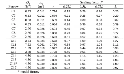
Scaling factors varied considerably between furrows reflecting the expected variability
(spatial, temporal and hydraulic) in the infiltration characteristic at the two sites. Differences
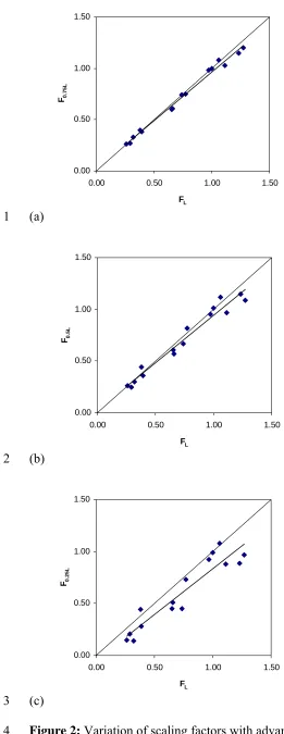
are also evident between the scaling factors at the various advance distances. These
differences are illustrated in Figures 1 and 2 for the Bura site and field C, respectively,
presented as plots of the scaling factor at each distance versus the values at the full advance
distance L. The assumption implicit in these plots is that the scaling factor at length L is the best estimate of the correct value of the scaling factor for the particular furrow.
Insert figures 1 & 2 about here
For each site the values of F at 0.75L and at L are almost identical. At 0.5L the values follow the 1:1 line but exhibit some small scatter about the line. By 0.25L the scaling factor values are showing considerable variation from the values at L. They no longer follow the 1:1 line and the scatter about the regression line is substantial. In the case of field C particularly,
some values of the scaling factor at 0.25L are much lower than expected. This is due to an apparently very rapid initial advance in some furrows giving an advance time to that point
being much less than that predicted by the fitted power curve. This may be attributed to an
initial unsteadiness in the furrow inflow, the effect of which diminishes for longer advance
distances (Bautista and Wallender 1993). This cannot be confirmed because full inflow
1
2
3
4
5
6
7
8
9
10
11
12
13
14
15
16
17
18
19
20
21
22
23
24
25
If the scaling process is to be used in a real time control system there is an obvious tension
between the desire to use an early advance point (to give adequate time for the subsequent
analyses) and the loss of accuracy in the scaled infiltration characteristics caused by the use
of that early advance point. The significant conclusion that can be drawn from these data is
that use of the mid-point (0.5L) is a reasonable compromise. Use of the point at 0.25L results in too great a loss of accuracy and should be avoided.
The nature of the variation of F with advance distance is determined entirely by the shape of the advance curve, as reflected in the value of the exponent r in the fitted power curve. When
r for a furrow is less than that for the model curve, that is, the advance exhibits lesser curvature than that for the model furrow, F increases with distance. This is seen, for example, at the Bura site (Table 3) for the furrows 13S 3 and 25S 2, and furrows C10 and
C11 (Table 4). When r is greater than that for the model furrow, F decreases with distance (furrows 9S 2, 31S 3, C12 and C15). This decreasing trend with distance is not as clear as the
previous increasing trend because, as has been seen earlier in Figures 1 and 2, the values at
0.25L tend to always be lower than the values at L. Trends with distance are also clearer for Bura where F was calculated from the fitted power curve compared to field C where the actual measured advance points were used. For those furrows where the r value is the same as or similar in magnitude to that for the model furrow, there is little or no change in F with distance (furrows 9S 3, 25S 1.5, C8 and C17). Any variation seen in these furrows is caused
by the extent of any deviation of the advance points from the smoothed advance curve.
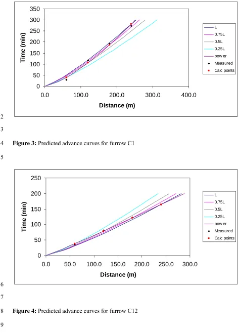
Figures 3 and 4 for furrows C1 and C12, respectively, provide an explanation for the above
behaviour. These plots show advance curves for these furrows calculated using the volume
0.5L, 0.75L and L. The measured advance points and the fitted power curve are also shown. In both cases the calculated advance curves are of slightly different shape from the actual
advance curve and intersect the actual advance curve at the advance point used to calculate
the scaling factor. Where r is lower than that for the model curve (furrow C1) the calculated advance curves lay mostly below the actual advance curve. The reverse applies when r is greater than that for the model curve. In both cases the curves predicted using F
1
2
3
4
5
6
7
8
9
10
11
12
13
14
15
16
17
18
19
20
21
22
23
24
25
L are closest to the measured advance curves. For furrows where r is the same as that for the model curve all of the advance curves (measured and predicted) coincide. This suggests that the
performance of the scaling process is entirely dependent upon the consistency of the shape of
the advance curves for a particular field or set of furrows.
Insert figures 3 & 4 about here
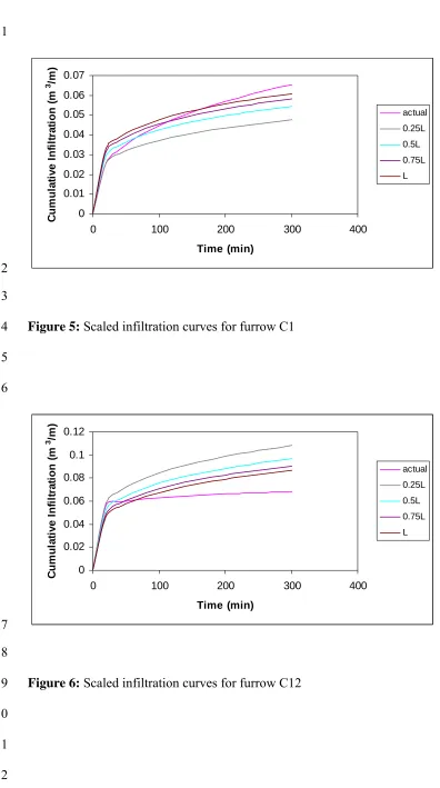
The effect on the predicted (scaled) infiltration characteristics is shown for the same two
furrows (C1 and C12) in Figures 5 and 6, respectively, in the form of plots of the scaled
infiltration curves superimposed over the actual curves as calculated by the INFILT program.
As would be expected from the above discussion the infiltration curves calculated using FL are closest to the actual infiltration characteristic. For the majority of furrows (where r is not far removed from that of the model curve) the scaled infiltration characteristics are much
closer to the actual or measured characteristic than the examples shown in Figures 5 and 6.
Insert figures 5 & 6 about here
1
2
3
4
5
6
7
8
9
10
11
12
13
14
15
16
17
18
19
20
21
22
23
24
25
if the scaled infiltration curve for a particular lay above or below the actual curve for that
furrow. Khatri and Smith (2006) argued that it was not necessary to model the infiltration
characteristic for each individual furrow with any great degree of precision. They suggested
that it was more important to provide a sufficiently accurate estimate of the spread or range of
infiltration curves for a field or set of furrows to allow best management of the field or set,
assuming that the flow rate and time to cut-off are the same for all furrows in the set. The
data presented in this paper suggest that if the scaling is performed using the advance to 0.5L
or later, then on average the scaling factors and hence the infiltration characteristics will be
sufficiently close to the correct values for practical purposes.
Scaling factor and wetted perimeter
Changes in wetted perimeter (or cross sectional area) with inflow rate, surface roughness or
slope are known to cause differences in the infiltration characteristic for a given furrow
(termed the hydraulic variability in this paper) and considerable work has been undertaken to
develop methods for adjusting infiltration to accommodate this source of variability. Use of
the scaling process of Khatri and Smith (2006) removes the need for any special adjustment
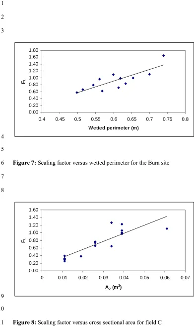
of the infiltration characteristic, the scaling factor F accounts for the effects of all forms of infiltration variability including the spatial, temporal and hydraulic. This is illustrated in
Figures 7 and 8.
Insert figures 7 & 8 about here
In Figure 7 the scaling factor at L is plotted against wetted perimeter for the Bura site. The
regression line (R2 = 0.687) suggests that nearly 70% of the infiltration variability observed at
spatial and temporal variability in the infiltration characteristic. Wetted perimeter data were
not available for site C. In this case the cross sectional area at the upstream end of the furrow
is used as a surrogate for wetted perimeter (Figure 8). Again the regression (R 1
2
3
4
5
6
7
8
9
10
11
12
13
14
15
16
17
18
19
20
21
22
23
24
25
2 = 0.741)
suggests that the hydraulic factors are responsible for a similar proportion of the infiltration
variability at this site.
Conclusion
Real-time control of furrow irrigation is the obvious way in which to overcome the effects of
the spatial, temporal and hydraulic variability in the soil infiltration characteristic and to
maximize irrigation performance. For this it is necessary to be able to obtain estimates the
infiltration characteristics for the furrows in real time and with the minimum of advance data.
In this paper a process is evaluated that uses scaling from a single advance measurement and
a model infiltration curve to give the infiltration characteristic for any other furrow in a field
or set of furrows.
Data from multiple irrigation events at two sites were analysed with scaling factors calculated
at 25, 50, 75 and 100% of the advance distance. The results showed that the calculated
scaling factors varied with distance down the furrow. The extent and nature of that variation
was shown to be a function of the shape of the advance curve as reflected in the power curve
parameter r, relative to that for the model curve.
It is concluded that any advance point used for scaling the infiltration should be taken at least
at the half way point down the field (0.5L). When used for real-time control this introduces a tension between the accuracy required from the scaling process and the desire to estimate the
1
2
3
4
5
6
7
8
9
10
11
12
13
14
15
16
17
18
19
20
21
22
23
24
25
The scaling process was applied to a series of furrows in which the inflow rate and slope
varied considerably, resulting in substantial variation in the wetted perimeter and hence in the
infiltration characteristic. Scaling factor was strongly correlated with the wetted perimeter
(R2 = 0.68 to 0.72) suggesting that the scaling is an appropriate way of both predicting and
accommodating the effect of the hydraulic variability. It is assumed that the remainder of the
variability in the magnitude scaling factor was due to the inherent spatial and temporal
variability in the infiltration of the soils at the two sites.
References
ASAE (2003) Evaluation of furrows. ASAE Standard EP419. American Society of
Agricultural Engineers, St. Joseph, MI
Bakker DM, Plunkett G, Sherrard J (2006) Application efficiencies and furrow irrigation
functions of irrigations in sugar cane in the Ord River Irrigation Area of North Western
Australia and the scope for improvement. Agricultural Water Management 83: 162-172
Bautista E, Wallender WW (1993) Reliability of optimized furrow infiltration parameters.
Journal of Irrigation and Drainage Engineering 119(5): 784-800
Camecho E, Lucena CP, Canas JR, Alcaide M (1997) Model for management and control of
furrow irrigation in real-time. Journal of Irrigation and Drainage Engineering 123(4):
264-269
Clemmens AJ (2000) Measuring and improving irrigation system performance at the field
level. Water - Essential for Life, Proceedings of Irrigation Australia 2000, Irrigation
Association of Australia National Conference and Exhibition
Dalton P, Raine SR, Broadfoot K (2001) Best management practices for maximising whole
1
2
3
4
5
6
7
8
9
10
11
12
13
14
15
16
17
18
19
20
21
22
23
24
25
Research and Development Corporation. National Centre for Engineering in Agricuture
Report 179707/2, USQ, Toowoomba
Gillies MH, Smith RJ (2005) Infiltration parameters from surface irrigation advance and
run-off data. Irrigation Science 24: 25-35
Khatri KL, Smith RJ (2005) Evaluation of methods for determining infiltration parameters
from irrigation advance data. Irrigation and Drainage 54: 467-482
Khatri KL, Smith RJ (2006) A real time control system for furrow irrigation to manage
spatial and temporal variations infiltration. Irrigation Science 25:33-43
McClymont DJ, Smith RJ (1996) Infiltration parameters from the optimization on furrow
irrigation advance data. Irrigation Science 17: 15-22.
Mailhol JC, Ruelle P, Povova Z (2005) Simulation of furrow irrigation practices (SOFIP): a
field scale modelling of water management and crop yield for furrow irrigation. Irrig Sci
24:37–48
Mwatha S, Gichuki FN (2000) Evaluation of the furrow irrigation system in the Bura
Scheme. Land and Water Management in Kenya: Towards Sustainable Land Use,
Proceedings of the Fourth National Workshop, Soil and Water Conservation Branch,
Ministry of Agriculture and Rural Development & Department of Agricultural
Engineering, University of Nairobi
Oyonarte NA, Mateos L, Palomo MJ (2002) Infiltration variability in furrow irrigation.
Journal of Irrigation and Drainage Engineering 128(1): 26-33
Raine SR, McClymont DJ, Smith RJ (1997) The development of guidelines for surface
irrigation in areas with variable infiltration. Proceedings of Australian Society of Sugar
Technologists 1997: 293-301
Rasoulzadeh A, Sepaskhah AR (2003) Scaled infiltration equations for furrow irrigation.
1
2
3
4
5
6
7
8
9
10
Sepaskhah, AR, Afshar-Chamanabad H (2002) Determination of infiltration rate for
every-other furrow irrigation. Biosystems Engineering 82(4): 479-484
Smith RJ, Raine SR, Minkovich J (2005) Irrigation application efficiency and deep drainage
potential under surface irrigated cotton. Agricultural Water Management 71(2): 117-130
Strelkoff TM, Souza F (1984) Modeling effect of depth on furrow infiltration. Journal of
Irrigation and Drainage Engineering 110(4): 375-87
Strelkoff TS, Clemmens AJ, Bautista E (2000) Field- parameter eestimation for surface
irrigation management and design. Watershed Management 105(142)
Walker WR (2001) SIRMOD II - Surface irrigation simulation, evaluation and design. User's
Table 1: Furrow characteristics for Bura Scheme (from Mwatha and Gichuki, 2000).
1
Parameter Value Furrow length 275-300m
Furrow spacing 0.9 m
Furrow slope 0.05 %- 0.3%
Cross-section parabolic Top-width (m)* T = 2.8y0.62
Wetted perimeter (m)* WP = 2.8y0.65
Area of flow (m2)* A = 1.48y1.55
* where y = furrow depth 2
3
4
5
6 7 8
Table 2: Advance curve parameters for the fifth irrigation at the Bura site
(from Mwatha and Gichuki 2000)
Advance parameters Irrigation Slope
(%)
Inflow
(ls-1) p r tL (mins)
1.5 12.7 0.49 572 2.0 6.1 0.67 308 0.09
3.0 10.2 0.57 345 1.5 12.6 0.56 262 2.0 11.3 0.57 290 0.13
3.0 18.3 0.53 177 1.5 13.5 0.56 231 2.0 22.2 0.46 256 0.25
3.0 16.2 0.61 110 1.5 16.5 0.55 179 2.0 17.9 0.53 186 5
0.31
3.0 13.4 0.68 90 9
1
2
[image:18.595.79.530.154.354.2]3 4
Table 3: Scaling factor F at different advance distances along the furrow for the Bura site WP Scaling factor F
Field
Qo (ls-1)
Ao
(m2) (m) r 0.25L 0.5L 0.75L L
9S 1.5 0.017 0.600 0.49 0.84 1.01 1.07 1.09
2 0.021 0.655 0.67 1.28 1.15 1.06 1.00
3 0.028 0.740 0.57 1.63 1.70 1.68 1.65
13S 1.5 0.015 0.568 0.56 0.39 0.56 0.61 0.62
2* 0.019 0.619 0.57 0.94 1.01 1.00 0.99
3 0.025 0.700 0.53 0.66 0.99 1.07 1.11
25S 1.5 0.012 0.514 0.56 0.58 0.65 0.66 0.66
2 0.015 0.561 0.46 0.50 0.80 0.90 0.96
3 0.020 0.634 0.61 0.68 0.81 0.83 0.83
31S 1.5 0.011 0.498 0.55 0.43 0.54 0.56 0.57
2 0.014 0.543 0.53 0.58 0.74 0.78 0.79
3 0.018 0.614 0.68 0.76 0.77 0.74 0.72
5
6 7 8 9
* model furrow inflow
Table 4: Scaling factor F at different advance distances along the furrow for the field C
Ao Scaling factor F
Furrow (lsQ-1o ) (m2) r 0.25L 0.5L 0.75L L
C1 0.83 0.011 0.714 0.15 0.26 0.26 0.26
C2 0.83 0.011 0.679 0.21 0.25 0.27 0.29
C3 0.83 0.011 0.639 0.14 0.30 0.33 0.32
C4 0.83 0.011 0.684 0.28 0.36 0.38 0.39
C7 2.60 0.026 0.694 0.45 0.67 0.74 0.74 C8 2.60 0.026 0.808 0.73 0.82 0.75 0.77 C9 2.60 0.026 0.693 0.51 0.57 0.61 0.66
C10 3.74 0.034 0.678 0.97 1.09 1.20 1.27
C11 7.92 0.061 0.730 0.88 0.97 1.03 1.11
C12 1.89 0.019 0.942 0.44 0.44 0.40 0.38
C13 3.80 0.034 0.728 0.45 0.61 0.60 0.65
C14 4.50 0.039 0.703 0.89 1.15 1.15 1.23 C15 4.50 0.039 0.850 1.08 1.12 1.08 1.06 C16* 4.50 0.039 0.808 0.99 1.01 1.00 1.00 C17 4.50 0.039 0.800 0.92 0.95 0.98 0.97 10
11
12
[image:18.595.64.494.448.706.2](a)
0.00 0.50 1.00 1.50 2.00
0.00 0.50 1.00 1.50 2.00 FL
F0.75L
1
(b)
0.00 0.50 1.00 1.50 2.00
0.00 0.50 1.00 1.50 2.00
FL F0.5
L
2
(c)
0.00 0.50 1.00 1.50 2.00
0.00 0.50 1.00 1.50 2.00 FL
F0.
25
L
3
[image:19.595.46.311.78.741.2](a)
0.00 0.50 1.00 1.50
0.00 0.50 1.00 1.50 FL
F0.75L
1
(b)
0.00 0.50 1.00 1.50
0.00 0.50 1.00 1.50 FL
F0.
5
L
2
(c)
0.00 0.50 1.00 1.50
0.00 0.50 1.00 1.50 FL
F0.25L
3
[image:20.595.45.306.74.749.2]1
0 50 100 150 200 250 300 350
0.0 100.0 200.0 300.0 400.0
Distance (m)
T
im
e
(
m
in
)
L
0.75L
0.5L
0.25L
pow er
Measured
Calc points
2
3
4
[image:21.595.47.520.100.760.2]5
Figure 3: Predicted advance curves for furrow C1
0 50 100 150 200 250
0.0 50.0 100.0 150.0 200.0 250.0 300.0
Distance (m)
T
im
e
(m
in
)
L
0.75L
0.5L
0.25L
pow er
Measured
Calc points
6
7
8
[image:21.595.65.521.103.343.2]9
1 0 0.01 0.02 0.03 0.04 0.05 0.06 0.07
0 100 200 300 400
[image:22.595.47.443.51.760.2]Time (min) C u mu la ti v e In filt ra ti o n ( m 3 /m) actual 0.25L 0.5L 0.75L L 2 3 4 5 6
Figure 5: Scaled infiltration curves for furrow C1
0 0.02 0.04 0.06 0.08 0.1 0.12
0 100 200 300 400
Time (min) C u mu la ti v e In filt ra ti o n ( m 3 /m) actual 0.25L 0.5L 0.75L L 7 8 9 10 11 12
1
2
3
0.00 0.20 0.40 0.60 0.80 1.00 1.20 1.40 1.60 1.80
0.4 0.45 0.5 0.55 0.6 0.65 0.7 0.75 0.8
Wetted perimeter (m)
FL
4
5
6
7
[image:23.595.46.441.73.728.2]8
Figure 7: Scaling factor versus wetted perimeter for the Bura site
0.00 0.20 0.40 0.60 0.80 1.00 1.20 1.40 1.60
0 0.01 0.02 0.03 0.04 0.05 0.06 0.07
Ao (m2)
FL
9
10
[image:23.595.64.441.158.363.2]