Validation of single spacecraft methods for collisionless
shock velocity estimation
Stefanos Giagkiozis1 , Simon N. Walker1 , Simon A. Pope1, and Glyn Collinson2
1Automatic Control and Systems Engineering, University of Sheffield, Sheffield, UK,2Heliophysics Science Division, NASA
Goddard Spaceflight Center, Greenbelt, Maryland, USA
Abstract
The velocity of a collisionless shock (CS) is an important parameter in the determination of the spatial scales of the shock. The spatial scales of the shock determine the processes that guide the energy dissipation, which is related to the nature of the shock. During the pre-ISEE era, estimations of relative shock-spacecraft velocity (VSh) were based on spatial scales of the shock front regions, in particularly thefoot. Multispacecraft missions allow more reliable identification ofVSh. The main objective of this study is to
examine the accuracy of two single spacecraft methods, which use the foot region of quasi-perpendicular shocks in order determineVSh. This is important for observational shock studies based on a single
spacecraft data such as Venus Express (VEX) and THOR, a proposed single spacecraft mission of European Space Agency. It is shown that neither method provides estimates with an accuracy comparable to multipoint measurements ofVSh. In the absence of alternative techniques to identify theVShand
therefore the spatial scales of the shocks, the methods can be used to provided order of magnitude estimations for the spatial scales of the shock front. Observations of the Venusian bow shock from VEX data have been used as an illustrative example for the application of these methods to estimate the shock spatial scale and the corresponding errors of this estimation. It is shown that the spatial width of the ramp of the observed shock isL∼3.4±1.4c∕𝜔pe.
1. Introduction
Collisionless shocks (CS) are wide spread in the universe. They are formed around ordinary stars, in binary systems, and are associated with gamma ray bursts. The key processes that take place in front of a CS are the transformation of the bulk flow energy of the plasma into thermal energy and the acceleration of a fraction of particles to very high energies. Important observational information about distant objects in the universe are received in the form of emissions. The source of these emissions is often particles thermalized or accelerated at the shock in the vicinity of the object. In spite of their common occurrence in the universe, only shocks in the heliosphere can be observed in situ. Heliospheric shocks include interplanetary shocks, planetary bow shocks, and the termination shock. One of the most important parameters of the shock is the spatial scale of the shock front. The spatial scale of the shock is related to the physical processes that coun-terbalance nonlinear steepening. The importance of the spatial scales of collisionless shock substructures is comprehensively discussed inKennel et al.[1985] andBalikhin et al.[1995]. The spatial scale of the shock (shock thickness) governs the interaction between particles and fields within the shock front. While adiabatic ther-malization of electrons is expected in the case of large shock front scales, a narrow shock front can lead to the effective overadiabatic electron thermalization [Balikhin and Gedalin, 1994;Gedalin et al., 1995]. The knowl-edge of the shock velocity with respect to the spacecraft is key for the estimation of the cross-shock potential [Formisano, 1982;Dimmock et al., 2012].
With the use of multipoint measurements provided by multispacecraft missions such as ISEE, Active Magnetospheric Particle Tracer Explorers (AMPTE), Cluster, and Time History of Events and Macroscale Inter-actions during Substorms (THEMIS), spatial and temporal ambiguity can be resolved. This allows the deter-mination of the speed of the shock relative to the spacecraft and hence the spatial scales of the shock front. Currently, only the terrestrial bow shock has been subjected to multipoint measurements, while planetary missions lack this ability. It is, however, important to study planetary bow shocks as they significantly expand the variety of shock parameters that are complementary to terrestrial bow shock data. For example, the detec-tion of a purely kinematic shock at Venus was reported [Balikhin et al., 2008], which has not been previously reported.
TECHNICAL
REPORTS:
METHODS
10.1002/2017JA024502 Key Points:• Comparison and accuracy evaluation of two single satellite methods used to estimate the velocity of collisionless shocks
• Neither method is comparably accurate to multispacecraft measurements
• One of the methods can potentially be used to determine the order of magnitude of the shock spatial width
Correspondence to:
S. Giagkiozis,
s.giagkiozis@sheffield.ac.uk
Citation:
Giagkiozis, S., S. N. Walker, S. A. Pope, and G. Collinson (2017), Validation of single spacecraft methods for collisionless shock velocity estimation,
J. Geophys. Res. Space Physics,122, doi:10.1002/2017JA024502.
Received 29 MAR 2017 Accepted 21 JUL 2017
Accepted article online 1 AUG 2017
©2017. The Authors.
In this study it is of interest to determine the accuracy of two proposed methods, one byMoses et al.[1985] and one byGosling and Thomsen[1985], which make use of the shock foot region to determineVSh, from single
spacecraft measurements. The foot region was first identified byWoods[1969], where it was shown that in front of supercritical, quasi-perpendicular shocks, the foot region is observed as a result of the reflected ions from the shock itself. When the angle between the normal vector to the shock surface (n) and the upstream magnetic field (Bu) is greater than 45∘, the shock is characterized as quasi-perpendicular. In supercritical CS,
the Mach number of the shock exceeds the first critical Mach number, above which anomalous resistivity cannot provide the required energy dissipation [Kennel et al., 1985].
Both methods use analytical expression for the width of the foot which combined with magnetic field obser-vations of the foot traversal time can yield an estimate of the relative to the spacecraft velocity of the foot. VShis then assumed to be the same, given that the foot structure will have the same velocity as the shock,
relative to the spacecraft. The accuracy of the estimates of the two methods mainly depends on the accu-racy analytical expression for the foot width.Moses et al.[1985] makes use of the analytical expression for the foot width derived byLivesey et al.[1984], where the result of the predicted foot width byWoods[1971] was generalized shock geometries other than perpendicular (𝜃Bn=90∘). On the other hand,Gosling and Thomsen [1985] defines the trajectory of the reflected ions in the deHoffman-Teller frame (HT) , where the solar wind velocity is parallel to the upstream magnetic field. The trajectories are then decomposed in parallel and per-pendicular directions of the magnetic field, and the foot width is defined by the distance covered by the ion, at the time of turnaround, i.e., the time when the velocity parallel to the shock normal, in the HT frame is zero. The calculation of the full particle trajectory offers a more complete and realistic analytical solution. The ana-lytical comparison of the two methods byGosling and Thomsen[1985] shows that the difference, of the foot width estimates, of the two methods will increase as𝜃Bndecreases.
The estimatedVShof the two methods is then compared with the measured velocity from two spacecraft Cluster measurements. In order to ensure that the velocity from two spacecraft is measured correctly, the main consideration to be taken is that the shock is not accelerating and that its geometry is not changing between the two observations. Therefore, the normal vector of the shock estimated by each of the two spacecraft must close and the separation between the two spacecraft must not be too large. Finally, the two spacecraft must not cross the shock simultaneously.
2. Instrumentation
Measurements of the terrestrial bow shock in this study were obtained from the Cluster spacecraft, launched in 2000, from the period 2012–2014. The four satellites initially had a highly elliptical orbit of about 4RE
perigee and 19REapogee, with an inclination of 90∘. The orbits of the four spacecraft have been modified several times, in order change the separation between the spacecraft. Throughout the course of the mis-sion, the orbit has evolved enabling greater coverage. The Cluster spacecraft orbit in a variable tetrahedron formation which ranges from about 10,000 km to 6 km distance between spacecraft. Magnetic field mea-surements were obtained from the Cluster Fluxgate Magnetometer (FGM) [Balogh et al., 1997], which offers data sampled at 22 Hz and 67 Hz in normal and burst mode, respectively. Measurements of the shock ion distributions were obtained by the time-of-flight Composition and Distribution Function analyzer (CODIF) of the Cluster Ion Spectrometry (CIS) experiment [R˙eme et al., 1997]. Finally, the Waves of High frequency and Sounder for Probing of Electron density by Relaxation (WHISPER) experiment [D˙ecr˙eau et al., 1997] was used to obtain the local electron plasma frequency in order to estimate the upstream plasma density. The review of Cluster data-based advances in the physics of quasi-perpendicular collisionless shocks is given inKrasnoselskikh et al.[2013].
3. Methodology
In this study we are concerned with the methods proposed byMoses et al.[1985] (method B) andGosling and Thomsen[1985] (method B) that use the width of the foot as observed by the spacecraft in order to determine the velocity of the shock. The foot of the shock is the region located upstream of the shock main ramp and is formed by gyrating ions reflected by the shock [Woods, 1969]. The foot appears in front of shocks that are of relatively low Mach number, supercritical and quasi-perpendicular.Moses et al.[1985] noted that if the length of the foot (dft) is known, then the traversal time of the foot (Δtft) is given by equation (1).
Δtft= dft
VSh±Vucos(𝜃Vn)
(1)
whereVuis the solar wind speed,VShis the shock speed in the normal direction, and𝜃Vnis the angle between
the solar wind and normal to the shock vector.Moses et al.[1985] then used the expression thatLivesey et al. [1984] developed to predict the width of the foot (dL
ft), assuming only specular reflection occurs (equation (2)).
dLft=0.68Vusin
2(𝜃
Bn)
𝜔ci
⋅n̂ (2)
After the correction noted byGosling and Thomsen[1985], the expression proposed byMoses et al.[1985] is given in equation (3).
VA
Sh=Vucos(𝜃Vn)
xL
1±xL (3)
where
xL=0.68
sin2(𝜃
Bn)
𝜔ciΔtft
(4)
𝜃Bnis the angle between the upstream magnetic field and the normal vector,𝜔ciis the ion cyclotron frequency,
andn̂is the shock normal.
Gosling and Thomsen[1985] used the deHoffman-Teller frame, in which theVu×Belectric field vanishes, to
obtain the expression in equation (5) for the foot width (dG
ft).
dG
ft=
Vu⋅n̂ 𝜔ci
f(𝜃Bn) (5)
where
f(𝜃Bn) =𝜔citot
(
2cos2(𝜃
Bn) −1
)
+2sin2(𝜃
Bn)sin(𝜔citot) (6)
cos(𝜔citot) = 1−2cos 2(𝜃
Bn)
2sin2(𝜃Bn) (7)
andtotis the time it takes for the ions to be overturned by the incoming solar wind after they are reflected and
all other quantities are the same as previously used. Applying the expression for the foot width in equation (5) in (1), the shock velocity is then given by equation (8) and (9).
VB
Sh=Vucos(𝜃Vn)
XG 1±XG
(8)
where
XG=
f(𝜃Bn)
𝜔ciΔtft
(9)
The positive sign is used for a downstream to upstream (outbound) transition of the shock and the negative for an inbound transition.
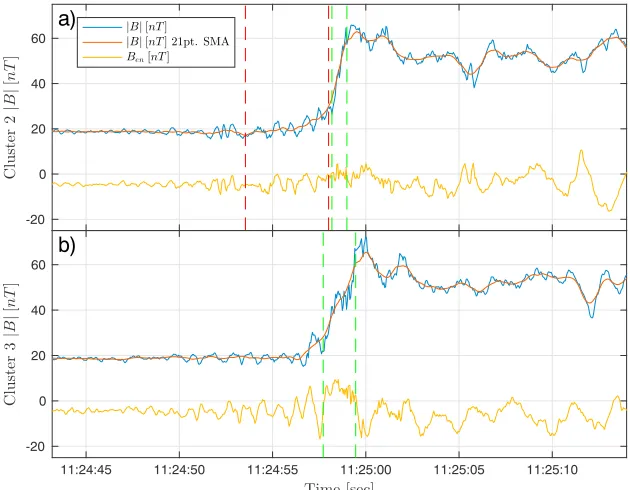
Figure 1.Magnetic field intensity plots recorded by (a) Cluster 2 and (b) Cluster 3 on 9 March 2012. The magnetic field profile of Cluster 3 has been shifted by about 34 s. The blue line is the measured magnetic field, the red line is the 21-point two sided simple moving average of the magnetic field, and the yellow line is the projection of the magnetic field to the normal vector. The vertical dashed red lines (Figure 1a) show the foot identified in the Cluster 2 observations. The vertical dashed green lines show the ramp identified for each spacecraft.
In order to compare the results of the two methods, the relative error (RE), defined in equation (10), will be considered.
RE=||V est Sh|−|V
obs Sh |
|Vobs Sh |
|×100% (10)
where Vest
Sh is the estimated velocity of the shock using the expressions of either A(equation (3)) orB
(equation (8)) andVobs
Sh is the shock velocity measured by the two spacecraft along the average normal vector
(navg) of the two spacecraft.
Given two vectorsa= [ax,ay,az]andb= [bx,by,bz], the average vector isab= [(ax+bx)∕2,(ay+by)∕2,(az+
bz)∕2]and the angle between them is given by𝜃ab=cos−1(a⋅b).
The normal of the shock is calculated using minimum variance analysis of the magnetic field (MVA). The eigenvectors of the magnetic variance matrixMnm =< BnBm>− < Bn> < Bm>, wheren,m = 1,2,3, are
orthogonal and correspond to the maximum, intermediate, and minimum variance directions of the mag-netic field. The eigenvector that associated with the smallest eigenvalue (i.e., minimum variance direction) corresponds to the shock normaln. The ambiguity of the direction of the eigenvectors in our case is solved by defining that the normals of the shock point toward the upstream region of the shock.
The MVA normals of the two spacecraft were limited to have a maximum angle of 25∘between them. The average normal is used for the calculation ofVobs
Sh , while forV est
Sh the normal vector of the spacecraft on which
the foot was observed is used. This will result to maximum 1−cos(12.5∘) = 0.0237, less than 3%, difference in the calculation ofVobs
Sh due to difference between the two normals used for the calculations.
4. Cluster Spacecraft Observed Shock Examples
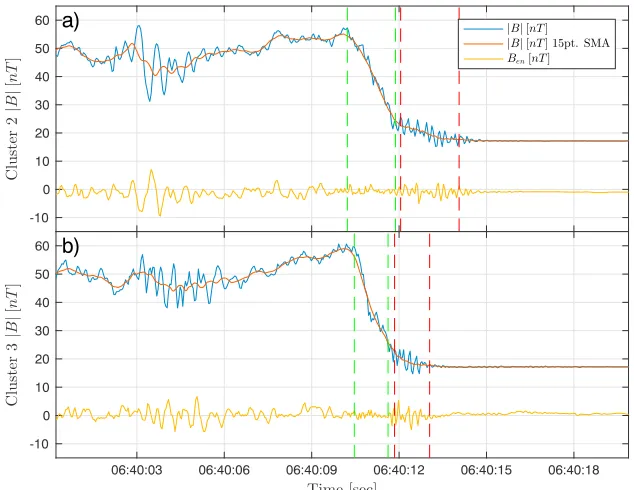
Figure 2.Magnetic field intensity plots recorded by (a) Cluster 2 and (b) Cluster 3 on 9 March 2012. The magnetic field profile of Cluster 3 has been shifted by about 33 s. The blue line is the measured magnetic field, the red line is the 15-point two sided simple moving average of the magnetic field, and the yellow line is the projection of the magnetic field to the normal vector. The vertical dashed red lines show the foot identified only in Cluster 2 (Figure 2a) and Cluster 3 (Figure 2b) observations. The vertical dashed green lines show the ramp identified for each spacecraft.
vectors for each pair was found to be less than 75∘, the event was kept. If no pair combination could be found with these conditions, the sample was discarded.
In Figures 1 and 2, the magnetic field intensity (blue solid line), the projection of the magnetic field along the normal vector (yellow solid line), and the two sided unweighted simple moving average ofNmeasured points (N pt. SMA) are plotted for each spacecraft for each of the pairs for the two examples. The main shock ramp is shown for each shock of Figures 1 and 2 between the green vertical dashed lines and the foot, where observed, is between the vertical dashed red lines.
The N pt. SMA was included to assist in the identification of the linear increase in front of the ramp that defines the foot. The two sidednpoint unweighted SMAx̂pfor a particular samplepis defined asx̂p= 1
n
∑n−1 2
i=−n−21xp+i,
wherexpis the measured value at samplepandnis odd. For the initial and final values where a sample does not exist, the measured value is assumed as 0. The number of points that are chosen depends on the magnetic field profile of the individual shock, with the consideration not to use too many points, because measurements from the downstream region will be combined with the foot. For example, if the measurements obtained from the Cluster instruments are sampled at 22 Hz. If the ramp of the shock is 3 s, then there will be 66 measure-ments of the ramp. If the filter is chosen to haveN = 45, then the average of the last point of the foot will include 22 points from the main magnetic ramp, which is one third of the ramp points. This will make the foot appear longer than it actually is, so a smaller window should be chosen.
4.1. Example 1: 9 March 2012 11:25 UT
The shock in this example was observed on 9 March 2012 by Cluster 3 (Figure 1b) at around 11:24:25 UT and 34 s later by Cluster 2(Figure 1a). The Cluster 2 measurements were offset by 34 s in the plot. The foot observed by Cluster 2 is marked in Figure 1a between the red dashed lines and was traversed inΔtft = 4.5s. Table 1
summarizes important parameters for the two shock observations. The average of the normals determined for each spacecraft wasnavg = [0.78,0.58,0.22], with an angle between the two normals 12∘. From the 34 s
time difference between the two observations and the spacecraft separation alongnavg,VShobs = 68km/s in
the spacecraft frame. Along the normal direction calculated from Cluster 2, the spacecraft where the foot was observed (Figure 1a), the two methods estimatedVA
Sh=47km/s (31% RE) andV
B
Table 1.Important Parameters, Values and Calculations for the First Example on 9 March 2012 (Figure 1)
Example 1: 9 March 2012
Spacecraft Cluster 2 Cluster 3
Time of crossing 11:24:58 UT 11:24:25 UT
r(103km) [70.57,−37.29,−31.32] [67.52,−39.94,−23.81]
rd(103km) [3.05, 2.65,−7.5]
Foot width (s) 4.5 Unclear foot identification
Normal [0.89, 0.44, 0.11] [0.64, 0.7, 0.32]
<Vu>(km/s) [−595.37, 5.46,−63.81]
<Bu>(nT) [−7.19, 7.43,−15.28] [−6.84, 7.11,−15.52]
𝜃Vn 26∘ 48∘
𝜃Bn 75∘ 76∘
𝜃rd<n> 74
∘
𝜔ci(rad/s) 1.8
-4.2. Example 2: 9 March 2012 06:40 UT
The second example is of a shock that was also observed on 9 March 2012 by Cluster 2 at 06:40:11 UT (Figure 2a) and by Cluster 3 at 06:40:44 UT (Figure 2b). Figure 2 follows the same formatting with Figure 1. A summary of the parameters of this example can be found in Table 2. The Cluster 3 time series was shifted by about 33 s. Using the average MVA normal of the two spacecraft [0.19, 0.92,−0.34],Vobs
Sh =162km/s.
The foot duration seen by Cluster 2 was 2 s (Figure 2 and Table 2) and along the Cluster 2 normalVA
Sh=23km/s
(86% RE) andVB
Sh=104km/s (36% RE). In this example both spacecraft observed a foot. The foot duration
observed by Cluster 3 was 1.3 s and along the normal estimated from the Cluster 3 magnetic field,VA
Sh=2km/s
(99% RE) andVB
Sh=178km/s (10% RE).
5. Statistical Results and Analysis
In total about 180 crossings of the four Cluster spacecraft were examined, about 720 individual shocks, using the previously mentioned considerations. The majority of the shocks were dismissed due to difficulty dis-tinguishing the foot region ahead of the magnetic ramp. An equally large number of pairs of shocks were dismissed due to disagreement between the normal vectors estimated for each of the spacecraft (𝜃n1n2>25
∘).
This resulted in 41 observations.
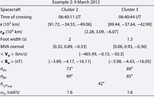
Table 2.Important Parameters, Values and Calculations for the Second Example on 9 March 2012 (Figure 2)
Example 2: 9 March 2012
Spacecraft Cluster 2 Cluster 3
Time of crossing 06:40:11 UT 06:40:44 UT
r(103km) [91.72,−34.55,−49.06] [89.44,−37.64,−42.99]
rd(103km) [2.28, 3.09,−6.07]
Foot width (s) 2 1.3
MVA normal [0.32, 0.89,−0.33] [0.06, 0.93,−0.36]
<Vu>(km/s) [−465.49,−0.15,−50.3]
<Bu>(nT) [−3.89,−4.17,−16.11] [−3.98,−4.43,−16.05]
𝜃Vn 73∘ 89∘
𝜃Bn 89∘ 85∘
𝜃rdnavg 42
∘
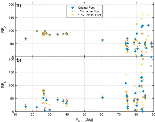
[image:6.612.242.510.574.747.2]Figure 3.RE for each of the 41 pairs of shock observations by the Cluster spacecraft, against the angle between the spacecraft separation vector and the shock normal direction (𝜃rdnavg). The RE of the estimates of (a) method A and (b) those for method B. Blue pluses show the RE using the foot as originally identified, the red crosses shows the RE of the same event using a 15% larger foot traversal time, and the yellow crosses for the 15% lower foot traversal time.
Figure 3 shows the RE of the 41 observations against the angle between the spacecraft separation vector and the average normal vector (𝜃rdn). The figure is in essence split in two parts, the measurements where𝜃rdn<70
∘
and the ones where𝜃rdn>70
∘. For the sample of the 41 observations, method A has an average RE of 153%
and a standard deviation of 215%, while method B has 113% and 165%, respectively. Due to the geometry of the spacecraft separation with the normal vector, it is not clear whether the large RE is caused by error in the measurement ofVShor due to error of the estimates of the two methods. On the other hand, for𝜃rdn <70∘ appear to have a better defined trend on their behavior. Keeping only the 14 points that have𝜃rdn<70
∘, the
average and standard deviation of the RE are 85% and 10% for method A and 41% and 24% for method B, respectively.
In order to take into account the effects of incorrect identification of the exact foot traversal time (Δtft), the
velocitiesVA ShandV
B
Shwere also calculated for a 15% larger and smaller foot traversal time. These estimates
are included in order to test the sensitivity of the two methods on the accuracy of the user to identify the correct foot traversal time. In Table 3, the quantities REOrefers to the RE when the original foot traversal time
(as identified by the data) was considered, while RELand RESrefer to the RE when the larger and smaller times.
The absolute difference of the RE from the original, defined as|ΔREOL|=|REO−REL|(for a larger foot) and
|ΔREOL|=|REO−REL|(for a smaller foot) were also calculated.
The measuredVShis also plotted against the estimates of both methods in Figure 4, where the blue crosses show the estimates of method A and the red circles the ones of method B for the 14 points where𝜃rdnavg<70
[image:7.612.174.575.698.744.2]∘.
Table 3.Summary of the Mean and Standard Deviation (SD) of the RE for Each of the Two Methods (A and B) for All Cases of Original (REO), Increased (REL) and Decreased (RES) Foot Width, and the Absolute Difference of the RE With the
Increase (|ΔREOL|) and Decrease (|ΔREOS|) of the Foot Width for the 14 Observations Where𝜃r
dn<70
Quantity REOA REOB RELA RELB RESA RESB |ΔREOLA | |ΔREOSA | |ΔREOLB | |ΔREOSB |
Mean 85% 41% 87% 44% 83% 42% 1.9% 2.6% 7% 13%
Figure 4.Estimated velocity against measured velocity using two spacecraft measurements for the 14 observations where𝜃rdn<70
∘.
The blue crosses represent the estimated velocity of method A, and the orange circles represent the estimated velocity of the method B. The diagonal blue dashed line represents shows the 0% error line, i.e., if the estimates agreed perfectly with the measured velocity.
Method A underestimates VSh for all cases substantially. A similar trend can be seen for method B as well, but some points are above the 0% relative error line.
Method B appears to be better suited to estimate the velocity of the shock using the foot width. It should be noted that perform better than method A, although the estimates in the sam-ple have a larger standard deviation. Looking at the estimates using the larger and smaller foot traversal times, method A appears to be more stable, but that is not necessarily good. On the contrary, it might indicate a flaw, because the actual traversal time does not appear to be as significant as for method B.
6. VEX Observed Shocks
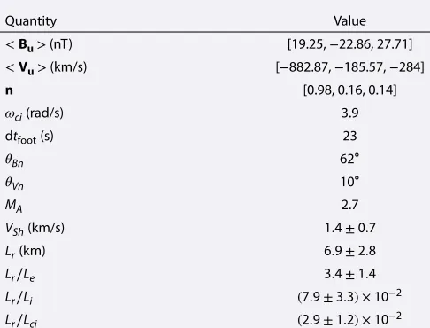
The following is one example from an observation of the Venusian by shock by VEX spacecraft on 5 November 2011 at about 7:00:22 UT. In Figure 5a the magnetic field intensity can be seen. The foot region identified is marked between the red dashed lines and can be seen that it begins where the upstream waves start to appear and a slight linear increase of the magnetic field magnitude begins to occur. The following three panels of the figure show the projection of the magnetic field vectors in the normal direction (en=n, Figure 5b), the vectorem=Bu×en(Figure 5c), and the vectorel=en×em(Figure 5d).
[image:8.612.218.531.451.697.2]Table 4.VEX Crossing on 5 November 2011 7:00:22 UT
Quantity Value
<Bu>(nT) [19.25,−22.86, 27.71]
<Vu>(km/s) [−882.87,−185.57,−284]
n [0.98, 0.16, 0.14]
𝜔ci(rad/s) 3.9
dtfoot(s) 23
𝜃Bn 62∘
𝜃Vn 10∘
MA 2.7
VSh(km/s) 1.4±0.7
Lr(km) 6.9±2.8
Lr∕Le 3.4±1.4
Lr∕Li (7.9±3.3) ×10−2
Lr∕Lci (2.9±1.2) ×10−2
The direction of the normal vector was determined using MVA of the magnetic field, with eigenvalue rations of 17.7 (maximum to intermediate) and 26.4 (intermediate to minimum). Along with the projection of the magnetic field along the normal vector, which appears constant throughout the ramp region (green vertical lines), the determination of the normal vector is considered to be accurate.
From the VEX measurements, the pro-ton temperature was measured at Tp ∼ 7.5 ×10⁵ K and the density at
dp∼6.8cm−3. The ion convective
gyro-radius was measured atLci ∼ 242km,
the electron inertial lengthLe ∼2km,
and the ion inertial lengthLi ∼ 87km.
For comparison, the Table 4 summarizes the quantities used for the calculation along with the estimate of method B for theVSh, the estimate of the spatial width of the shock ramp (Lr) and how it compares withLe,Li, andLci. The shock is quasi-perpendicular and supercritical; therefore, the methods can be applied. The solar wind velocity of this shock is large due to a CME that was observed before the crossing, which leads to a large ion convective gyroradius. The average magnetic field is large, which leads to a small electron gyroradious.
7. Discussion and Conclusions
The final set of observations is small in count, compared to the initial number of shock crossings that were considered, but we believe it to be a representative sample for both methods, mainly due to the certainty of the measuredVShusing two spacecraft. The statistical results indicate that neither of the two methods is
comparably accurate with the two spacecraft measurements ofVSh. Method B [Gosling and Thomsen, 1985]
appears to be more accurate in the determination ofVShand also has a larger standard deviation the changes of the foot traversal time, which could indicate that the analytical expression that determines the spatial width of the shock foot region is more appropriate, since it does affect the estimate more. This also means that when method B is used, greater care must be taken in the identification of the foot traversal time.
Based on the example of from the Venusian bow shock, method B can be used to determine that the scales of the shock is of the order of magnitude of c
𝜔pe .
References
Balikhin, M., and M. Gedalin (1994), Kinematic mechanism of electron heating in shocks: Theory vs observations,Geophys. Res. Lett.,21(9), 841–844.
Balikhin, M., V. V. Krasnoselskikh, and M. Gedalin (1995), The scales in quasiperpendicular shocks,Adv. Space Res.,15(8–9), 247–260. Balikhin, M. A., T. L. Zhang, M. Gedalin, N. Y. Ganushkina, and S. A. Pope (2008), Venus express observes a new type of shock with pure
kinematic relaxation,Geophys. Res. Lett.,35, 1–5, doi:10.1029/2007GL032495.
Balogh, A., et al. (1997), The Cluster Magnetic Field Investigation, inThe Cluster and Phoenix Missions, pp. 65–91, Springer, Dordrecht, Netherlands.
Barabash, S., et al. (2007), The Analyser of Space Plasmas and Energetic Atoms (ASPERA-4) for the Venus Express mission,Planet. Space Sci.,
55(12), 1772–1792.
D ˙ecr ˙eau, P. M. E., P. Fergeau, V. Krannosels’kikh, M. L ˙ev ˙eque, P. Martin, O. Randriamboarison, F. X. Sen ˙e, J. G. Trotignon, P. Canu, and P. B. Mögensen (1997), WHISPER, A resonance sounder and wave analyser: Performances and perspectives for the cluster mission,
Space Sci. Rev.,79(1/2), 157–193.
Dimmock, A. P., M. A. Balikhin, V. V. Krasnoselskikh, S. N. Walker, S. D. Bale, and Y. Hobara (2012), A statistical study of the cross-shock electric potential at low Mach number, quasi-perpendicular bow shock crossings using Cluster data,J. Geophys. Res.,117, A02210, doi:10.1029/2011JA017089.
Formisano, V. (1982), Measurement of the potential drop across the Earth’s collisionless bow shock,Geophys. Res. Lett.,9(9), 1033–1036. Gedalin, M., K. Gedalin, M. Balikhin, and V. Krasnosselskikh (1995), Demagnetization of electrons in the electromagnetic field structure,
typical for quasi-perpendicular collisionless shock front,J. Geophys. Res.,100, A69481.
Gosling, J. T., and M. F. Thomsen (1985), Specularly reflected ions, shock foot thicknesses, and shock velocity determinations in space,
J. Geophys. Res.,90, A109893.
Acknowledgments
Kennel, C. F., J. P. Edmiston, and T. Hada (1985), A quarter century of collisionless shock research, inCollisionless Shocks in the Heliosphere: Reviews of Current Research, pp. 1974–1979, AGU, Washington, D. C.
Krasnoselskikh, V. V., et al. (2013), The dynamic quasiperpendicular shock: Cluster discoveries,Space Sci. Rev.,178(2–4), 535–598. Livesey, W. A., C. T. Russell, and C. F. Kennel (1984), A comparison of specularly reflected gyrating ion orbits with observed shock foot
thicknesses,J. Geophys. Res.,89, A86824.
Moses, S. L., F. V. Coroniti, C. F. Kennel, F. L. Scarf, E. W. Greenstadt, W. S. Kurth, and R. P. Lepping (1985), High time resolution plasma wave and magnetic field observations of the Jovian bow shock,Geophys. Res. Lett.,12(4), 183–186.
Pope, S. A., T. L. Zhang, M. A. Balikhin, M. Delva, L. Hvizdos, K. Kudela, and A. P. Dimmock (2011), Exploring planetary magnetic environments using magnetically unclean spacecraft: A systems approach to VEX MAG data analysis,Ann. Geophys.,29(4), 639–647.
R ˙eme, H., et al. (1997), The Cluster Ion Spectrometry (CIS) Experiment, inThe Cluster and Phoenix Missions, pp. 303–350, Springer, Dordrecht, Netherlands.
Vaivads, A., et al. (2016), Turbulence Heating ObserveR: Satellite mission proposal,J. Plasma Phys.,82(5), 905820501.
Woods, L. (1969), On the structure of collisionless magneto-plasma shock waves at super-critical Alfvén-Mach numbers,J. Plasma Phys.,3, 435–447.
Woods, L. C. (1971), On double-structured, perpendicular, magneto-plasma shock waves,Plasma Phys.,13(4), 289–302.
Zhang, T. L., et al. (2006), Magnetic field investigation of the Venus plasma environment: Expected new results from Venus Express,