BigSUR: Large-scale Structured Urban Reconstruction

White Rose Research Online URL for this paper:

http://eprints.whiterose.ac.uk/138594/

Version: Accepted Version

Article:

Kelly, T orcid.org/0000-0002-6575-3682, Femiani, J, Wonka, P et al. (1 more author)

(2017) BigSUR: Large-scale Structured Urban Reconstruction. ACM Transactions on

Graphics, 36 (6). 204. ISSN 0730-0301

https://doi.org/10.1145/3130800.3130823

© 2017 Copyright held by the owner/author(s). Publication rights licensed to Association

for Computing Machinery. This is the author's version of the work. It is posted here for your

personal use. Not for redistribution. The definitive Version of Record was published in ACM

Transactions on Graphics, https://doi.org/10.1145/3130800.3130823. Uploaded in

accordance with the publisher's self-archiving policy.

[email protected]

https://eprints.whiterose.ac.uk/

Reuse

Items deposited in White Rose Research Online are protected by copyright, with all rights reserved unless

indicated otherwise. They may be downloaded and/or printed for private study, or other acts as permitted by

national copyright laws. The publisher or other rights holders may allow further reproduction and re-use of

the full text version. This is indicated by the licence information on the White Rose Research Online record

for the item.

Takedown

If you consider content in White Rose Research Online to be in breach of UK law, please notify us by

TOM KELLY,

JOHN FEMIANI,

PETER WONKA,

NILOY J. MITRA,

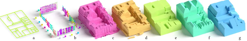
Fig. 1. Structured Urban Reconstruction.Given street-level imagery, GIS footprints, and a coarse 3D mesh (let), we formulate a global optimization to automatically fuse these noisy, incomplete, and conflicting data sources to create building footprints (middle: colored horizontal polygons) with profiles (vertical ribbons shown for several footprints) and atached building façades (vertical rectangles). The output encodes a structured urban model (right) including the walls, roof, and associated building elements (e.g., windows, balconies, roof, wall color, etc.). Inset below: A reference aerial image.

The creation of high-quality semantically parsed 3D models for dense met-ropolitan areas is a fundamental urban modeling problem. Although recent advances in acquisition techniques and processing algorithms have resulted in large-scale imagery or 3D polygonal reconstructions, such data-sources are typically noisy, and incomplete, with no semantic structure. In this paper, we present an automatic data fusion technique that produces high-quality structured models of city blocks. From coarse polygonal meshes, street-level imagery, and GIS footprints, we formulate a binary integer program that globally balances sources of error to produce semantically parsed mass mod-els with associated façade elements. We demonstrate our system on four city regions of varying complexity; our examples typically contain densely built urban blocks spanning hundreds of buildings. In our largest example, we pro-duce a structured model of 37 city blocks spanning a total of 1,011 buildings at a scale and quality previously impossible to achieve automatically.

CCS Concepts: ·Computing methodologies→Scene understanding; Shape analysis;Mesh models; ·Applied computing→Architecture (build-ings);

Additional Key Words and Phrases: urban modeling, structure, reconstruc-tion, façade parsing and element classiicareconstruc-tion, procedural modeling

Permission to make digital or hard copies of all or part of this work for personal or classroom use is granted without fee provided that copies are not made or distributed for proit or commercial advantage and that copies bear this notice and the full citation on the irst page. Copyrights for components of this work owned by others than the author(s) must be honored. Abstracting with credit is permitted. To copy otherwise, or republish, to post on servers or to redistribute to lists, requires prior speciic permission and⁄or a fee. Request permissions from [email protected].

© 2017 Copyright held by the owner⁄author(s). Publication rights licensed to Association for Computing ℧achinery.

0730-0301⁄2017⁄11-ART204 $15.00 https:⁄⁄doi.org⁄10.1145⁄3130800.3130823

ACM Reference format:

Tom Kelly, John Femiani, Peter Wonka, and Niloy J. ℧itra. 2017. BigSUR: Large-scale Structured Urban Reconstruction.ACM Trans. Graph.36, 6, Arti-cle 204 (November 2017), 16 pages.

https:⁄⁄doi.org⁄10.1145⁄3130800.3130823

1 INTRODUCTION

Obtaining detailed 3D urban models is important for a variety of applications ranging from urban planning and environmental simulations to virtual reality and video game creation. Given the importance of such

mod-els, extensive eforts have been undertaken to cre-ate polygonal meshes from aerial images or light de-tection and ranging (Li-DAR) scans. Such datasets are often very expensive and tedious to create. They are diicult to use because they are typically heteroge-neous with sparse or

miss-ing details. ℧ore importantly, they lack semantic structure, which prevents easy use in subsequent applications.

a b c d e f g

Fig. 2. Baseline methods.(a) GIS footprints represent plot ownership more accurately than building structure. (b) Image features, such as windows (cuboids) extracted from street-level imagery, are available only near where the images have been taken (cubes), and lack information about the interior of the structure; diferent images may give contradictory features for the same building. (c) Raw polygonal meshes tend to be more complete, but they contain noise and are typically polygon soups. One reconstruction possibility is to fit horizontal ªfloorsº to the mesh (d), while another is to extrude the GIS footprints to heights available from a database (e). Both these approaches fail to convey the roof structures of the input. A popular GIS data visualization techniques is to create a

hip roofover all footprints (f), which leads to a monotonous structure. (g) Naively applying profiles from the input mesh to the GIS footprints leads to more

interesting roof shapes; but these are inaccurate because the GIS edges are frequently not representative of real-world building walls.

vertical proiles to create mass models by extruding the footprint upwards along the proiles, which may then be ‘decorated’ with building elements such as windows, doors, etc. Currently, this work-low is suitable for coarse approximation of larger areas, or for detailed manual modeling of particular (iconic) buildings, but it does not scale to accurate detailed modeling of wider urban areas. In this paper, we focus on the problem of procedurally creating structured models by leveraging data from multiple sources (see Figure 1 and the inset aerial view for reference). Such raw informa-tion has diferent strengths and weaknesses: for example, publicly availableGeographic Information System footprints(GIS footprints) carry reliable records of plot ownership, but they often do not re-lect built reality; polygonal meshes, often in the form of polygon soups obtained by processing aerial images, provide coarse informa-tion, but they lack semantic partitioning or ine details; street-level imagery (e.g., façade photographs) provides detailed information, but it lacks 3D information or semantic labels. Further, each data source has its own coordinate system, sufers from distortion, and frequently contains mutually conlicting or partial information.

Naively combining information across the above datasources results in various types of artifacts (see Figure 2). For example, extruding GIS footprints with proiles extracted from mesh data creates misleading mass models, while transferring window loca-tions regressed from images onto estimated façade planes results in poorly positioned windows.

Instead of heuristically combining the above datasources, we propose a uniied fusion algorithm. We develop an optimization formulation that analyzes the heterogeneous data sources (i.e., GIS footprints, polygonal meshes, and street-level imagery) and retargets them to a single consistent representation. By balancing the various retargeting costs, our algorithm reaches a consensualstructured model, the output of which is building-level footprints, associated proiles along the footprint boundaries, and façade elements placed appropriately over the mass models (see Figure 1). The raw input data to our algorithm comes from various preferred layout directions (extracted from GIS information), candidate building footprints and proiles (extracted from the polygonal meshes), and façade parti-tions with associated elements (extracted by analyzing the individual façade images). Our system automatically decideswhichof these

elements to retain andhowto adapt the selected elements to create consistent output. Figure 15 shows the input GIS footprints and the extracted building footprints produced by our algorithm. We note that the result is semantically structured in the sense that the output has labels associated with the diferent sections of the output model (e.g., windows, balconies, shops, walls, roofs, etc.). Further, our algorithm doesnotmake ℧anhattan-world assumptions, nor does it restrict the roof angles (i.e., roofs can be lat or sloped), nor number of pitches (i.e., façades can alternate an arbitrary number of times between wall and roof).

We demonstrate the efectiveness of our system by evaluating four difering urban settings:Detroitas a suburban US city with simple detached houses,New Yorkwith blocks of near-regular high-rise buildings arranged on a (literal) ℧anhattan-grid,Oviedoas a typical historic European city with non-axis aligned buildings surrounding inner courtyards, andLondonwith dense urban architecture with many annexes and complex roof shapes. Finally, we semantically reconstruct a very large area of central London covering 37 blocks around Oxford Circus and compare our method with state-of-the-art urban reconstruction techniques.

In summary, we introduce a novel wide-area fusion algorithm that semantically combines multi-channel, noisy, and conlicting in-formation to produce structured models in the form of building mass models with associated façade elements. We demonstrate the auto-mated method on urban neighborhoods spanning several building blocks at a scale that has not been previously demonstrated.

2 RELATED WORK

We review the relevant literature on the urban modeling and recon-struction pipeline (see [℧usialski et al. 2013] for a survey).

2.1 Reconstructing mass models

2006] or dense [Ceylan et al. 2013; Furukawa and Ponce 2010] point clouds. Some integrated modeling pipelines extract mass models from images directly [Dick et al. 2004; Garcia-Dorado et al. 2013; Vanegas et al. 2010]. Surface models can be extracted from point clouds, e.g., by resampling onto a grid [Poullis and You 2009], 2.5D contouring [Zhou and Neumann 2010], relation-based primitive itting [℧onszpart et al. 2015], or Poisson reconstruction [Kazhdan and Hoppe 2013]. Another important component in urban model-ing is segmentation [e.g., Golovinskiy et al. 2009; ℧atei et al. 2008; Verdie et al. 2015] to separate buildings from other classes.

Our work is mainly related to shape abstraction and simpliica-tion; we aim to create simple and plausible mass models from noisy input data. One simple model for shape abstraction is to regular-ize the models using the ℧anhattan-world assumption [Li et al. 2016]. Alternately, very good results can be achieved by itting parametric building blocks to height ields [Lafarge et al. 2010] or LiDAR input [Lin et al. 2013], exploiting non-local regularity re-lations [Zheng et al. 2010], or obtaining depth-layer rere-lations by jointly analyzing images and LiDAR scans [Li et al. 2011b]. Fol-lowing Verdie et at. [2015], we use a noisy building mesh as input. They use a simpliied version of Globit [Li et al. 2011a] to detect relationships between extracted planes to regularize the output. In contrast to this method, we jointly analyze the diferent input data modalities to produce a consistent structured model, in which, for example, the footprints of the mass models are in agreement with how the street-level imagery is partitioned into diferent buildings.

2.2 Façade parsing

The goal of façade parsing is to extract façade elements such as win-dows, doors, and balconies. The input of façade parsing is typically a single image or a point cloud. A typical initial step of façade parsing is to compute local per-pixel information, such as segmentation information [℧artinović et al. 2012], edge detection, or symmetry detection [℧üller et al. 2007]. This input is then regularized to make it more compliant with a given model of a façade structure [Cohen et al. 2014]. One possible model is a grid with one spacing parameter for each row and each column [℧üller et al. 2007], which can also be represented by a rank-one matrix [Yang et al. 2012]. A more general model is a hierarchical splitting tree, in which each internal node splits into multiple horizontal or vertical slices [Dai et al. 2012; Kozinski et al. 2015; Riemenschneider et al. 2012; Shen et al. 2011; Teboul et al. 2013]. These hierarchical approaches difer in how they incorporate low-level features stemming from classiiers and in how they use encoded architectural knowledge. Example solutions include use of ℧RFs [Kozinski et al. 2015], extending the CYK algo-rithm [Riemenschneider et al. 2012], application of reinforcement learning [Teboul et al. 2013], post-processing by optimization [Jiang et al. 2016; ℧artinović et al. 2012; Nan et al. 2015], or jointly opti-mizing for template matching and deformation estimation [Ceylan et al. 2016]. A signiicant simpliication used by these systems is to consider only façade images that have been rectiied and cropped for individual buildings.

Section 4

℧esh

Section 4.2 & 6 Section 5.3

B Images

S&C Section 5.1 GIS

Optimization

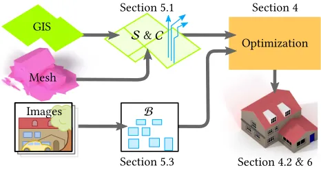
Fig. 3. Overview.Starting from GIS footprints, a coarse 3D mesh, and street-level imagery, we extract a set of sweep-edges,S, a set of clean-profiles, C, and a set of building-façades,B. These are then globally optimized to produce a semantically parsed building block as output.

2.3 Interactive reconstruction

To achieve improved results, another line of work investigates in-teractive techniques for mass modeling [Debevec et al. 1996], or façade parsing. For example, Nan et al. present an interactive façade modeling system for LiDAR data [2010] and Xiao et al. propose an interactive system for images [2008]. Another recent concept is to train multiple neural networks to interactively create procedural models from input sketches [Nishida et al. 2016]. In contrast, we aim to create an automatic system.

In this work, we build on the geometry of the straight skele-ton [Aichholzer et al. 1996] to model architecture. Early work used theunweightedstraight skeleton to model roofs [Laycock and Day 2003; ℧üller et al. 2006] and walls [Fang et al. 2013]. Theweighted skeleton [Eppstein and Erickson 1999] ofered enhanced expres-siveness; in particular, theprocedural extrusionsystem (PE) [Kelly and Wonka 2011] consisted of stacked weighted skeletons. Recently, Biedl et al. [2016] reinforced the theoretical underpinnings of the weighted straight skeleton, renewing our interest in PEs. Essentially, PEs are a parameterization of architecture into a horizontal 2D plan with a set of vertical 2D proiles that are associated with the edges of this plan. Such a parameterization can represent buildings with arbitrarily angled walls and roofs to provide a strong architectural prior. In this work, we develop a method to project real-world data into the space of buildings represented by PEs.

3 PROBLEM SETUP

Fig. 4. Terminology.Let: The data are used to create street-level imagery with associated façade planes (orange), raw-profiles (blue) and sweep-edges (pink). Center: These are processed to create the input to the optimization Ð a smaller set of clean-profiles (blue), building-façades (orange lines), and building-façade-points (orange points), and a ground plane tessellation consisting of sweep-edges (pink) and sot-edges (black) enclosing faces. Right: The output of the optimization is a collection of watertight footprint-polygons (pink and purple), with a clean-profile assigned to every edge, and positions for every building-façade (orange).

3.1 GIS footprints

Typically, an urban building block consists of several densely packed buildings (up to 100 buildings in our examples). While GIS foot-prints (see [℧iller et al. 2017]) provide an accurate ownership record, surprisingly they provide little usable information concerning a building’s physical walls and partitions, making it challenging to use these data directly for reconstruction. However, we found that they carry a mixture of accurate and noisy orientation information, which we utilize to regularize the processing of other data sources.

3.2 Coarse 3D mesh

A 3D mesh or polygon soup (e.g., obtained via multi-view stereo or LiDAR scans) provides approximate, incomplete, noisy, but large-scale geometric information. We process such meshes to produce two entities: horizontalsweep-edgesand verticalclean-proiles(see Figure 4); such sweep-edges are extruded along clean-proiles to create a mass model. Speciically, we extract a set of lines, referred to as sweep-edges,S, on the ground-plane by identifying likely façades over the mesh. Along these sweep-edges, we vertically slice the mesh to create manyraw-proiles; these are clustered, averaged, and abstracted to create asetofclean-proiles,C(see Figure 4 and Section 5.1). Direct reconstruction from these sweep-edges and clean-proiles is challenging as PEs require watertight footprint-polygons, with a clean-proile assigned to each edge. Speciically, there are two sources of diiculty: the sweep-edges have gaps, may self-intersect, or even be missing entirely in regions, while the clean-proiles are the output of local analysis, thus lacking information about building partitions and containing diferent sources of noise (e.g., from initial reconstruction, trees, or vehicles).

3.3 Street-level façade images

Complementary to the above data sources, street-level imagery provides information over portions of the urban blocks. Such im-ages typically come with estimates of camera position and orienta-tion. For each image, we use a convolutional neural network (CNN) based supervised classiier (see Section 5.3) to detect the rectangular bounds of a façade as well as elements such as windows, doors, and balconies. We refer to this rectangular façade containing a col-lection of extracted elements as abuilding-façade(see Figure 4).

Each side of a city block will typically consist of multiple overlap-ping building-façades: one from each of the images. However, such raw building-façades,B, may contain position and orientation er-rors, have inconsistent scales, sometimes overlap, or be incomplete (e.g., occluded by trees, vehicles, or scafolding). The ground plane location of the observed start or end of a building-façade in the street-level imagery is referred to as abuilding-façade-point.

These three data sources are in three diferent coordinate systems, and may introduce conlicting information, making their combina-tion challenging. Further, each is subject to reprojeccombina-tion and inherent noise, both within and between datasets. For example, we found that the given location and orientation of building-façades varied on diferent sides of a building due to GPS or GIS errors. Poor cor-relation between the image and 3D mesh was sometimes observed because of difering scale estimates or changes in the environment (e.g., buildings had been constructed, modiied, or demolished).

3.4 Notation

Before we formulate the main binary integer program (BIP) that processes these inputs, we irst introduce some notation. We use sweep-edges,S, to oversegment the ground plane (y=0) to form a

tessellation of faces,G_{, as described in Section 4.1. Our algorithm}

determines whether or not each edge,e_k∈G_{, should be selected,}

thus implicitly encoding the inal building footprint-polygons. We represent this selection with a binary indicator variable,sk, such thatsk=1 if the edge,ek, is selected and forms part of a footprint-polygon, andsk =0 otherwise. Note that in densely built urban

areas, even though adjacent buildings can share a common wall, the structures often have diferent heights or roofs. We encode such a situation by two, possibly diferent, proiles associated with the two sides of each interior wall,ek. (For the remainder of the paper, we discuss one such proile per edge, while the other one is similarly treated.) We denote the length of any edge,e_k, as∥e_k∥ and the maximum mesh height above a point on the ground plane, (x,z)∈R2_{, ash(x},z).

We use logic operators (such as∧,∨,⊕,¬) noting that each can be expressed in BIP constraints with additional variables (detailed in Appendix A). We will not explicitly introduce such extra variables and constraints, but we use the logic operator directly.

Unlikesk, which is an individual binary variable, we will have cause to represent categorical variables (such as color or proile choice) usingselection vectors. Note they are also called ‘one hot vectors’ in the literature. We denote a selection vector of lengthn

asχ:=(χ1, . . . ,χn); each element (such asχ1) is a binary variable. Selection vectors haveexactlyone element set to one, while the others are all zero. We encode this condition with the constraint Pn

i=1χi =1.We will wish to compare two selection vectors. For example, givenχ:=(χ1...χn)andψ:=(ψ1...ψn), we desire an out-put of 0 if all elements are equal (i.e.,χi =ψi, ∀i), and 1 otherwise. To simplify notation in this situation, we writeisDifferent(χ,ψ) to indicate

a b c d

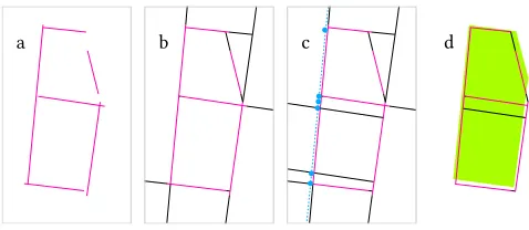
Fig. 5. Sweep-edges and soft-edges.A set of sweep-edges (a, pink) are ex-tended to oversegment the ground plane (b) into faces. The sweep-edges are inserted one at a time, in order of decreasing length. To complete the tes-sellation, the sweep-edges are extended bysot-edges(black). The building-façade-points (c) further subdivide the ground plane if there are no existing similar edges. Finally, we remove faces that are mostly outside the GIS footprint (d, green) to create the tessellation,G_.

4 FUSION OPTIMIZATION

So far, we have introduced: (i) a set of sweep-edges,S(for extraction details see Section 5.1); (ii) a set of clean-proiles,C(Section 5.1); and (iii) a set of building-façades,B(Section 5.3). We continue to formulate a global optimization that fuses these entities to out-put a semantically parsed building block, simply referred to as the structured model(see Figure 3).

To achieve this, we address three key challenges: (i) identifying footprint-polygonsfor each building in the ground plane tessellation; (ii) selecting a clean-proile fromCfor each edge of every footprint-polygon; and (iii) retargeting building-façades fromBto a subset of the edges of the footprint-polygons. A good building-façade location matches the mass models that are implicitly obtained by extruding the footprint-polygons along the selected clean-proiles.

Note that the above problems are tightly linked and must be solved together. For example, the boundary of a footprint-polygon depends on which proiles are selected, which in turn depends on how the building-façades are retargeted to match 3D mass model boundaries.

4.1 Formulation

We simultaneously address the above challenges by formulating a BIP; we next describe the optimization variables, constraints, and objective terms associated with each challenge.

4.1.1 Identifying footprint-polygons. The input GIS footprints,

street-level imagery, and 3D mesh carry noisy and incomplete infor-mation about individual buildings. This is particularly pronounced in densely built urban areas where adjacent buildings often share walls, contain courtyards, and regularly break the ℧anhattan-world assumption. Using the available information, we irst oversegment the ground plane intofacesusing the sweep-edges, then merge the oversegmented regions, and inally extract the footprint-polygons. First, we extend the sweep-edges inSto initiate the ground plane oversegmentation (see Figure 5a). Note that only the edges created by sweep-edges have proiles, while others, calledsoft-edges, complete the tessellation (see Figure 5b). Next, we use the estimated building-façade-points (shown as blue dots in Figure 5c) from the

Fig. 6.Oversegmenting the ground plane.We use sweep-edges and GIS foot-prints to overpartition the ground plane. Let: The sweep-edges (pink) along with their sot-edge extensions (black) partition the plane. Center: Further oversegmentation based on the building-façades extracted from street-level imagery (blue). Right: using height and GIS information (green) we identify the interior faces to produce the oversegmentation,G_.

street-level imagery to further oversegment the ground plane by adding soft-edges that are perpendicular to the building-façade into the tessellation. All these edges indicate potential separating walls between adjacent buildings. Finally, we discard faces that are either mostly outside the GIS footprints, or have a mean mesh height below a threshold (3m in our data). We useG_{to denote the resulting}

tessellation (see Figure 5d).

Extracting footprint-polygons amounts to setting the BIP vari-ables,sk, for each of the edges,e_{k, surrounding every face,fi} ∈G_.

However, setting up such an optimization is cumbersome, as not all values for{sk}result in valid partitions of the ground plane (see Figure 7). Hence, we indirectly formulate the problem by deciding which neighboring faces in the tessellationG_{should be merged}

to produce the inal building footprint-polygons. For example, the resulting tessellation for Figure 1 is shown in Figure 6.

The footprint-polygons should ideally follow the sweep-edges, while making them watertight, and should use as few soft-edges as possible to ill in sections of missing data. Further, we encourage selection of edges where there is a large height diference on either side of a sweep-edge (e.g., between adjacent buildings). For each such facefi ∈G, we sampleh(x,z)using the mesh data to ind the mean height over the face,h(fi). This averaging adds robustness over problematic mesh features such as holes. The height diference across an edge is thusheightDif(e_k)₌|h(fi)−h(fj)|wherefiand

fjare the faces incident toek.

a

b

c

Selection variables:The face-merging problem can be reduced to a region- (or map-) coloring problem with adjacent faces of the same color indicating that the faces are implicitly merged. Thus, for each

fi, we assign a selection variable,γi, with length 5. Although four colors are suicient for map-coloring, we found experimentally that our BIP converges faster with an extra color.

Constraints:The edge-selection variable,sk, deines if an edge,ek, lies on a footprint-polygon; usually this is because it lies between faces of diferent colors. Thus, for all edges,e_k, between two faces

fi andfj, we require

sk =isDifferent(γi,γj),

which amounts to a set of variables and constraints as introduced in Section 3.4. Since all other edges,e_{k, are at the boundary and must} be part of a footprint-polygon, we set theirskto 1.

Objective terms:In formulating the selection of edges from the tes-sellation,G_{, we add penalties for the following conditions: (O1) if a}

sweep-edgeis notselected or a soft-edgeisselected; and (O2) if an edge with high height diferential isnotselected

O1({sk}):=

X

e_k∈G

2∥e_k∥(¬sk∧isSweepEdge(e_k))

+

X

e_k∈G

∥e_k∥(sk∧ ¬isSweepEdge(e_k))

O2({sk}):=

X

e_k∈G

∥e_k∥heightDif(e_k)¬sk,

whereisSweepEdge(e_k)returns 1 if the edge,e_k, is a sweep-edge, or 0 if it is a soft-edge.

4.1.2 Selecting clean-profiles.The input mesh data are noisy,

incomplete, and often contain spurious geometry (e.g., trees or cars). Our goal is to abstract the raw input by assigning a clean-proile from the set,C, to everye ∈ G_{. These assigned proiles guide}

the footprint-polygon extrusion, implicitly producing a clean and abstracted PE mass model.

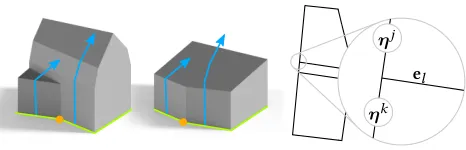
Ideally, above each edge, the selected proile closely approximates the mesh geometry. Further, due to stability considerations when modeling with PEs, it is important that edges from adjacent and nearly parallel edges in the same footprint-polygon select the same proile (see Figure 8). Note that this caveat does not require buildings to conform to the ℧anhattan-world assumption.

Selection variables:For every edge,e_{k, we create a proile selection} vector,ηk, to indicate which clean-proile is selected from the global set,C. The length of this vector is the size of the proile set,C, typically 4-80 proiles.

Constraints:We wish clean-proile selections to be equal for parallel adjacent edges within the same footprint-polygon. In other words, two adjacent edges that are nearly parallel can select diferent pro-ilesonly ifthe they belong to diferent footprint-polygonsÐ i.e., there is at least one separating wall between them.

Thus, for all vertices of the tesselation,G_{, we create an auxiliary}

variable for each pair of adjacent and approximately parallel (we use a tolerance of 0.1 radians) edges,e_jande_{k, as}

r(j,k) =isDifferent(ηj,ηk).

ηj

e_l

ηk

Fig. 8. Undesirable façade splits.Let-center: PEs are unstable when diferent profiles (blue) are selected on nearly parallel edges (green); moving a single point (orange) a short distance creates a very diferent result. Right: To avoid this situation, the clean-profiles of the adjacent parallel edges (given by the selection vectorsηj andηk) are constrained to be equal, if the dividing edge is selected (sl=1).

Because we allow only parallel and adjacent edges to have diferent proiles (r(j,k) =1) when there is at least one selected edge (sl =

1 for edgee_l) between them at their shared vertex (Figure 8), we require

r(j,k) ≤ X e_l∈between(j,k)

sl,

wherebetween(j,k)denotes the set of edges lying betweene_jande_k and sharing a common vertex. We implementG_{as a half-edge data}

structure, which permits direct implementation of thebetween() operator.

Objective term:For each edge,e_k, let the corresponding set of raw-proiles obtained by vertically slicing the input mesh beR(e_{k). Let} the vectorF_k list the error in itting each clean-proile,pc ∈ C, to all the raw-proiles,q ∈ R(e_{k), along the edge,}e_{k. This error} is measured by the functiond(), which measures the diference between two proiles (see Section 5.1 for details). Speciically, each element of the vector,F_kc, is computed for a single clean-proile,

pc∈ C, over all the edge’s raw-proiles as

F_kc=

X

q∈ R(e_k)

d(pc,q,minY(q),maxY(q)).

Note that for the above computation,pc is moved to align with

qat heighty =0 (i.e., on the sweep-edge). Further, the function

d()is evaluated over the raw-proile’s height, [minY(q),maxY(q)], to match raw-proiles with ends at varying heights to the more complete clean-proile. If there is no raw-proile associated with an edge, we set the assignment cost vector,F_{kto [}−1,0, . . .0], i.e., we give a small bonus to selecting the vertical clean-proile. (Note that the -1 favors the default vertical proile in the absence other information.) We can now deine an objective term for each edge, e_k, measuring the it of the selected clean-proile to the supporting edge’s raw-proiles,

O3({ηk}):=

X

e_k∈G

∥e_k∥F_k·ηk.

4.1.3 Retargeting building-façades. Street-level imagery of façades contains valuable information about building placement. For exam-ple, neighboring buildings may have diferent materials which pro-vides evidence about their widths, or a change in façade height may advocate splitting a footprint-polygon. However, street-level im-agery often does not align with the 3D mesh (or even other images) Ð both in position and scale. We extend our formulation to include such street-level imagery by observing that solving for alignment and scaling is equivalent to establishing correspondence between the start and end building-façade-points, and the vertices on the boundary of the tessellation.

Speciically, let the set of vertices on the outer boundary ofG_be V_{. We aim to assign every building-façade-point to a vertex,v∈}V_.

Because the error in the building-façade location is of a known maximum distance (approximately 3m in our datasets), we can enumerate the nearby boundary vertices for each point. In the process, we aim to minimize both the façade-point displacement and the height disparity between the building-façade-based (street-level imagery), and mesh-based, estimates. We note that multiple images may create overlapping building-façades, with each suggesting a corresponding set of façade elements. Selection variable:We cluster nearby building-façade-points to a group,C_{i, with a cluster-representative denoted bym}i

⋆. For each cluster-representative, we ind the nearby boundary vertices in

V_{, denoted asnearby(m}i

⋆). We use a selection variable,τ

(i,w)_{, to}

identify the points inC_{i mapped to vertexvw.}

Objective terms:We introduce three terms: (O4) to discourage stretch and height disparities between heights extracted from the mesh and those from the street-level imagery; (O5) to encourage building-façade-points to pick exterior corners of the tessellation; and (O6) to reduce splitting of footprint-polygons under a building-façade.

First, to minimize stretch and height disparity of the building-façades (see Figure 9), we add

O4({τ(i,w)}):=

X

∀Ci X

ma∈Ci X

w∈nearby(mi

⋆)

τ(i,w)(distance(vw,ma)+

|htLeft(ma)−htLeft(vw)|+

|htRight(ma)−htRight(vw)|),

where the functiondistance()gives the distance between a boundary vertex and building-façade-point, andhtLeft()gives the building-façade height or face height (from the street-level imagery or the 3D mesh, respectively), on the left (similarly forhtRight()), as shown in Figure 9.

It is particularly desirable to assign a building-façade-point to a corner vertex of the tessellation boundary (a subset ofV_{); thus, it}

receives a reward

O5({τ(i,w)}):=− X vw∈corners

τ(i,w),

where the setcornercontains all vertices adjacent to two boundary edges ofG_{that meet at [π}/3,2π/3].

m1,2,3 v1 |htLeft(ma)−htLeft(vw)|

|htRight(ma)−htRight(vw)|

distance(vw,ma)

C_i

v2

Fig. 9. Stretch and height disparity.Let: We evaluate the fit of the building-façade (blue) to the 3D mesh (grey) using stretch and height disparity. Right: The building-façade-points,m1,m2,m3, are grouped into a cluster,Ci, with

representativemi

⋆. The indicator variableγ

(i,1)_(orγ(i,2)_{) denotes which} of the points in clusterC_{iare mapped to the boundary vertex,v1(orv2).}

Finally, it is undesirable for an edge to be selected that arrives at the tessellation boundary underneath a building-façade (in-set: top, blue). Such an edge may unnec-essarily split a footprint-polygon (pink). Hence, we penalize the selection of edges, e_k, that approach vertices of the boundary with building-façades, but without selecting building-façade-points. This results in im-proved integration of the façade boundaries into the mass model (inset, bottom). Specif-ically, we penalize such a situation as

O6({lk}):=

X

e_k∈G

sk∧lk.

Constraints:The auxiliary binary variable,lk, captures whether a vertex of edge,e_k, is not assigned a building-façade-point, but is covered by a building-façade,

lk =

X

vw∈verts(ek)

*. ,

free(vw) X

∀C_i

τ(i,w)+/

-<1.

The above constraint evaluates whether an edge,ek, has a boundary vertex,vw ∈verts(ek), which is covered by a building-façade, but is not assigned a building-façade-point by anyτ. The functionfree(vw) returns 0 if the vertex,vw, is covered by some building-façade and 1 otherwise.

4.1.4 Objective function.We ind a solution that satisies all the

above constraints, while minimizing

min 6 X

i=1

αiOi

over the variables{γi},{ηk},{τ(i,k)}, and the associated auxiliary variables. In our results, we usedα1=10,α2=1,α3=0.01,α4=1,

andα5=α6=0.1P

Fig. 10. Overlapping building-façade elements.An urban block is typically covered by multiple overlapping façade images, giving repeated bounding rectangles for many elements, such as windows (turquoise), shops (pink), balconies (orange), doors (green), mouldings (dark blue), and building-façade boundaries (light blue). The let-most visible facade of Figure. 1 was recon-structed from these overlapping elements.

4.2 Creating the Structured Model

Given asolutionto the above optimization, we can generate the geometry for the inal structured model.

Starting from the ground plane tessellation,G_{, and the region}

coloring{γi}, we merge neighboring faces to which the solution assigns the same color. The resulting 2D polygons form the polygons of the inal mass models. For every edge in each footprint-polygon, the solution contains a clean-proile from the setC, in{ηk}. Procedural extrusions [Kelly and Wonka 2011] lift each footprint-polygon using the selected clean-proiles to create a building’s mass model. During this extrusion, we cap the PE mesh at the average mesh height (sampled byh(x,z)over the footprint-polygon) to stop runaway geometry and to create lat roofs. An exception is when the PE horizontal cross-section area is decreasing rapidly at this height, in which case we assume that the roof is pointed. We cap pointed roofs at a higher level given by the average raw-proile height around the footprint-polygon boundary. We classify the surfaces obtained via PE as walls or roofs using the local normals. The optimization solution assigns the building-façades to portions of the mass-model. This correspondence between building-façade-points and vertices of the footprint-polygons is given by{τ}; from this, we can position the building-façades over the mass models.

The building-façade’s points are found from image features. One, or both, points may be missing because they lie outside the image. If both points are present, we translate and scale the building-façade to align its building-façade-points with the corresponding footprint vertices. If only one point is present, we simply translate it to align with the found vertex. In the case of no points, the building-façade is aligned using estimated Google StreetView (GSV) pose data.

In this manner, multiple building-façades can be positioned over the same section of the mass model, giving us multiple position estimates for façade elements (doors, windows, balconies etc., see Figure 10). Further, because these elements have been estimated from street-level imagery, they contain noise and omissions.

In the following, we explain our fusion and regularization process for window elements, while other element classes (doors and bal-conies, etc.) are treated similarly. We adopt a simple mean-shift [Fuku-naga and Hostetler 1975] approach; at each iteration, we apply a step of 0.2×the mean-shift vector to all window rectangles for a variety of parameterizations. Namely: (i) absolute position of the left, right, top, and bottom of the rectangle (to align windows with themselves and others in a grid); (ii) width and height (to maintain

the shape of the windows in subsequent iterations); and (iii) spacing between adjacent windows to the left, right, top and bottom (to en-courage uniform spacing between windows). After the mean-shift has converged (we use 30 iterations), we frequently have multiple rectangles associated with each window. Such rectangles are merged if the overlap is more than 50%; otherwise, the smallest rectangles are discarded. Element rectangles are also discarded if they occur in less than half of the street-level images that cover them.

These element rectangles are added to the mass model using simpleparametric modelsfor each type of element, such as windows, doors, window-sills, cornices, moldings, and balconies. These are parameterized to the found dimensions, and windows or doors are recessed into the mass model façade. As an exception, windows that lie on a mass model surface that is classiied as a roof, or between surfaces with diferent normals, are added as dormer windows.

Finally, we color the mass model polygons classiied aswallusing the information extracted from the street-level imagery, and those classiied asroofusing optional satellite image information. Figure 1 shows such a resulting structured model.

5 IMPLEMENTATION DETAILS 5.1 Extracting Sweep-edges and Profiles

We now describe the proile analysis of the 3D mesh and GIS foot-prints. First, we align the mesh with the GIS footprint boundary. Then, we create and clusterhorizontal-lines(Figure 11b, c) to ind theprominent-facesof the building-block (Figure 11d). Each such face is used to compute asweep-edgeon the ground plane, along which we extract verticalraw-proilesfrom the mesh (Figure 11e). The proiles are processed to create a small, yet representative, set ofclean-proiles,C.

First, we align the mesh to the GIS footprints using the GPS position associated with the mesh. We use the GIS footprint bound-ary to discard mesh geometry more than a street-lane width away (typically 4m) from the building-block of interest.

We found horizontal-lines to be good indicators of predominant directions in architectural meshes; they also support the strong horizontal edges that are characteristic of PEs. To ind such lines, we slice the mesh horizontally (we used 20cm intervals), and simplify each such slice using polyline itting (Figure 11a). Because the mesh may have holes and noise, we use the directions in the GIS footprints to regularize the line itting (Figure 11b). Speciically, if lines are within 20◦_{of the closest GIS edge, they are rotated to match the GIS} line’s orientation.

a b c d e

Fig. 11.Sweep-edges and proile analysis.A horizontal slice of the mesh (a, orange), has polylines fited to it (b) and is regularized by the GIS information (b, green). These are clustered from the seed-lines (c, bold lines), and the associated prominent-faces (d), which can be used to find the raw-profiles (e).

The prominent-faces are now sampled to obtain proiles (Fig-ure 11d). Aproileis a weaklyy-monotone polychain (i.e., every point is greater, or equal, in height to every preceding point). This monotonic property is required by PEs, which we observe is satis-ied by a large majority of building types. We continue to extract a set of raw-proiles directly from the 3D mesh; the mesh is sliced per-pendicularly to the seed-line’s direction at regular intervals (20cm). Nearly horizontal mesh faces (with a normal approximately 5◦_from vertical), or those not associated with the prominent-face are ig-nored. We create a raw-proile by traversing a portion of the slice, starting at the closest point on the slice to the prominent-face’s seed-line. The traversal takes place upwards and downwards, select-ing monotonic line-segments from the slice to add to the proile. It jumps over small gaps and non-monotonic sections of the slice by searching for the next point in a small locale (approximately 2m).

We now use the raw-proiles to ind a smaller, yet representative, set of clean-proiles,C. We irst cluster the raw-proiles along each sweep-edge using proile distance. Given two monotone proiles,pi andpj, we deine the proile diference at a height,y, as

δ(pi,pj,y)=

   

q

(x(pi,y)−x(pj,y))2+4(∠(pi,y)−∠(pj,y))2 ifpiandpjare deined at height y, 10 otherwise.

Fig. 12. Raw- and clean-profiles.Let: Each color represents a cluster of adjacent and similar profiles from Figure 1. Right: A cluster of raw-profiles (grey) has line segments fited to it (purple) and is finally regularized to yield a clean-profile (blue).

wherex(pi,y)and∠(pi,y)are, respectively, the x-position and an-gle (in radians), of proilepiat heighty. When the proiles range between heightsyl andyu, the cumulative distance function is then the mean horizontal distance between the proiles discretized over the vertical range [yl,yu] as

d(pi,pj,yl,yu):=

X

y∈[yl,yu]

δ(pi,pj,y)/(yu−yl).

The raw-proiles are clustered by examining consecutive proiles along each sweep-edge, starting a new cluster whenever

d(plast,pnext,0,maxY(plast,pnext))>t,

wheretis a threshold value and maxY(pi,pj)is the maximum height of proilespi andpj. Small clusters with fewer than ive proiles are discarded. Empirically, we ind that forming clusters from such contiguous portions of sweep-edges gave better results than tech-niques such as spectral clustering, because it prioritizes the strong spatial-correlation between adjacent raw-proiles. Examples of such clusters are shown in Figure 12-left.

To create a simpliied clean-proile from each cluster of raw-proiles, we it a set of line segments (Figure 12-right). Using strong architectural priors, we regularize these lines into a clean-proile. Because of the low resolution of our input meshes, we found we could aid regularization by requiring the proiles to be both verti-callyandhorizontally monotonic (note that PEs require only that the proiles be vertically monotonic).

We used the following rules to create the clean-proiles (see Fig-ure 12-right): (i) lines that are nearly horizontal or vertical are snapped to these orientations. Near the ground, this snapping is very aggressive to mitigate the efect of occluders; (ii) lines that do not form part of vertically and horizontally monotonic proiles are either removed or sliced so that they do; (iii) lines that are near the ground are extended to the ground; and, inally, (iv) if two adjacent lines could be extended to intersect within 2m of an end of both lines, we extend the lines to this intersection. We add the resulting clean-proile to the proile set,C.

Positive NegativeEdge Ignored

Fig. 13. Training data and façade classiication.Top-let: The ground truth used to for the ‘Façade' and ‘Window' labels. Remainder: The source image (top-right) used to compare a model trained to recognize a single set of disjoint labels (botom-let) with one trained to recognize independent sets of labels for each type of feature with edge labels (botom-right). Each model was trained for 150 Epochs. The second option leads to crisper features.

Finally, for each prominent-face, we compute a sweep-edge. Sweep-edges repre-sent potential wall posi-tions over the ground plane, and, along with suitable vertical clean-proiles,

cre-ate the 3D mass models. We ind a sweep-edge by projecting the seed-line of each prominent-face onto the ground plane (inset; or-ange line), and ofsetting it to lie close to the start of the proiles (inset; pink line). This ofset is necessary because the found seed-line may not be on the structure’s wall. The ofset is the mean horizontal distance from the seed-line to the bottom of the raw-proiles. This set of sweep-edges,S, represents the potential wall-positions.

5.2 Acquiring Street-level Imagery

We use street-level imagery from Google StreetView (GSV) to esti-mate the locations of façade elements such as windows, balconies, doors, and moldings, as well as the locations of façade boundaries. Unprocessed GSV images are 360◦_{panoramas including} approxi-mate pose data (position and orientation of the rig used to capture the images) that are estimated using GPS and a variety of additional techniques described by Anguelov et al. [2010]. Based on the GSV pose information and GIS footprints, we project the GSV panorama images onto the expected façade plane to obtain a (roughly) rectiied projected image.

These projected images are generated at a resolution of 40 pixels ⁄ meter. We crop the images to a ixed horizontal ield of view of 120◦. This is centered on the projection of the paranorama center onto the façade plane. We use a ixed ield of view to avoid distortion caused by projecting the panorama at extreme angles. This results in more than one overlapping image of each façade and many images containing only a portion of a façade. We note that some façades have no GSV images because of legal and physical constraints on photography. A typical example of missing imagery is the private courtyards found in the center of many European city blocks. Next, we describe how to ind façade features in the projected images.

µ

µ+σ

Fig. 14. Finding façade extents.Let: We split images with multiple façades based on the peaks of the vertical sums of the façade ‘Edge' scores that are output by the segmenter (superimposed in blue over the image); façades are split at the highest point of each interval where the projection's value is more than one standard deviation (σ) above its mean (µ). Right: The integral of the detected 'Sky' label (green) is used with a threshold to identify the top of the façade.

5.3 Analyzing Street-level Imagery

Starting from input street-level imagery, our goal is to detect each façade’s location and dimension, and its building elements (e.g., windows, balconies, etc.). Abuilding-façaderecords this information for one image and one estimated façade; we refer to the set of building-façades asB.

In practice, we found the GSV pose estimates to be insuicient to produce projected street-level imagery that is suiciently aligned with GIS data. In the example of London, we observed overlaid GSV imagery to deviate from GIS building footprints by nearly 3m on the façade plane, or 5◦ in GSV panoramas. Therefore, a pre-processing step removes parts of the images that are unlikely to be part of a façade and then rectiies each image. The unwanted features are segmented and masked-out using theBayesian SEGNET CNN [Badrinarayanan et al. 2017; Kendall et al. 2015]. This network was trained on urban street scenes using CamVid data [Brostow et al. 2008] and then reined using CityScapes data [Cordts et al. 2016] to identify parts of images that are likely to have façade features. We then rectify based on the edges within that region using the method proposed by Afara et al. [2016].

Next, we identify the façade elements within these rectiied im-ages. We reine the probabilistic Bayesian SEGNET architecture to segment a set of labels for architectural façade element features using the C℧P Facade dataset [Tylecek 2012], the dataset used by Afara et al. [2016], and an additional dataset of 800 facades that we annotated directly from GSV images of London, Oviedo, and New York. We use this SEGNET-FACADE model (available at: https:⁄⁄github.com⁄jfemiani⁄facade-segmentation) to assign per-pixel probabilities to the images for each feature class.

Fig. 15. Oviedo, Manhattan, and London.City blocks from Oviedo (let, center-let), Manhatan (center-right) and London: Litle Portland Street (right, as Figure 1). Top: Our results. Botom: input GIS footprints (green) and optimization output floorplans (blue). See also Table 1.

and one for the façade extent itself. Each task assigns one of four labels to each pixel; ‘Negative’, ‘Positive’, ‘Unspeciied’ (which is ignored), or ‘Edge’. The ’Edge’ label is automatically assigned to a thin region (6 pixels spanning an estimated 15cm) around the edge of each feature, with the exception of vertical façade edges, where the ‘Edge’ label is assigned to a wider region (15 pixels wide, spanning approximately 38cm). Using a separate ‘Edge’ label ensures more weight is given to the training-loss in these pixels due to median frequency balancing [Eigen and Fergus 2015]. Empirically, these improvements result in sharper features, as shown in Figure 13, which is useful for isolating individual feature instances. The CNN processes images at a resolution of 512×512 pixels. We rescale all images to a height of 512 pixels and crop the widths. During inference, several horizontal tiles are used to cover an image.

The GSV images often contain multiple façades, and it is impor-tant to separate them into diferent individual building-façades for the optimization. At the inference stage, we sum each pixel col-umn’s Bayesian SEGNET-FACADE scores for the ‘Edge’ label. This one-dimensional signal peaks at each façade boundary. The signal is dilated by 60 pixels (1.5m) in order to merge the dual-peaks that can occur if the street-level imagery is imperfectly rectiied, or if there are stitching artifacts (see Figure 14). We extract peaks as local maxima that are more than one standard deviation above the mean of the dilated signal (see Figure 14-left). Each façade image is split at these peaks to producebuilding-façades. For each building-façade, we produce axis-aligned bounding boxes of all features as shown in Figure 14-right. In order to estimate the height of each building-façade, we use the original SEGNET to label pixels as ‘Sky’. The 85th percentile of the scores at each pixel-row forms a one dimensional sky signal (see the green region of Figure 14-right). The top of the façade is the lowest point where the sky signal crosses 50%. These width and height estimates are assigned to each building-façade and

used in the optimization stage. Because we know the location of the façade image-plane inR3_{, the building-façade has an estimated 3D}

position, as do the associated features.

5.3.1 Training and Evaluation.We trained SEGNET-FACADE on

80% (1173 images) of the data we collected, an additional 20% (293 images) were used to evaluate the precision, recall, andF1-scores of our approach. SEGNET-FACADE obtained a per-pixel precision of 96%, recall of 69%, and anF1of 0.80. By comparison SEGNET trained on the same data obtained a per-pixel precision of 73%, recall of 62% and anF1of 0.67. We also evaluated per-object precision by deining a successful match between objects as an intersection-over-union over 50%. The per-object scores gave a precision of 88%, recall of 68%, and anF1score of 0.77. We consider these to be useful results as many of the façade images were collected łin the wildž from GSV and imperfectly rectiied. In comparison, SEGNET acheived precision of 36% and recall of 28%, with anF1of 0.32. The recent method of Afara et al. [2016] had a per-object precision of 85%, recall of 52%, and anF1score of 0.64 on the same data.

5.3.2 Collecting color estimates.Although a façade may contain

Fig. 16. London: Oxford Circus blocks.Structured urban reconstruction spanning 37 blocks and 1,011 buildings.

6 RESULTS

We implemented the proposed framework using Java and Python; the sourcecode is available online at the project page (http:⁄⁄geometry. cs.ucl.ac.uk⁄projects⁄2017⁄bigsur). We used Gurobi [Gurobi 2016] for binary integer programming and Cafe [Jia et al. 2014] for the CNN-based classiication. The timings were recorded on an i7-7700K desktop (with the exception of the Oxford Circus example).

We demonstrate our framework on building blocks from diferent cities: Detroit (see Figure 17), ℧anhattan and Oviedo (see Figure 15), and London (see Figure 1 for Little Portland Street and Figure 16 for Oxford Circus). We selected building blocks to show a variety of inputs, from free standing single-family houses in Detroit to dense urban areas in the other three selected cities. We selected cities with

Table 1. Details for Figure 15. Values are given for location, number of clean profiles (| C |) and sweep edges (| S |), binary variables (vars) and constraints (constr), number of output footprints (fp), and the solve times.

Fig:col location |C| |S| vars constr fp solve

(lat,long) out time

15:1 43.36635, 75 61 32,242 73,193 34 15h -5.83256

15:2 43.36584, 73 56 74,694 148,945 38 5h -5.83189

15:3 40.72191, 46 30 23,172 49,941 37 4h -74.00131

1:1 51.51724, 58 60 45,249 88,171 28 4h 15:4 -0.14199

Table 2. Details for Figure 17, columns as in Table 1.

Fig:row location |C| |S| vars solve

(lat,long) time

17:1 42.38458, 9 5 196 0.01s -82.95086

17:2 42.38458, 8 7 657 0.05s -82.95084

17:3 42.38587, 6 4 165 0.00s -82.95165

17:4 42.38614 23 13 1,799 2.92s -82.95125

17:5 42.38350, 37 14 1,494 0.3s -82.94954

accessible mesh and GIS data. In our experiments, we found most of the parameters to be stable when the input data quality remained consistent. Typically, we adjusted two parameters before running the optimization: the thresholds for the creation ofG_{and the mesh}

area for ignoring small clusters of horizontal lines. These parameter adjustments are relatively interactive because they occur before the slow BIP optimization.

6.1 Timings

The computation times are dominated by the time it takes to com-pute a solution to the binary integer program. We list details of this optimization for selected blocks in Tables 1 and 2. Other compo-nents that contribute to the runtime are image processing to extract building-façades (about 45 seconds per image), mesh processing to extract sweep-edges and clean-proiles (less than 20 seconds per block), grid-based regularization of façade elements (less than 3 seconds per façade), basic mass model construction (less than 10 sec-onds per block), and façade element insertion into the mass models (less than 10 seconds per block).

6.2 Comparison

We compared our work to other related algorithms in Figure 19. As there exists no competing work to fuse multiple data sources, we limited our comparison to the processing of mass models. Therefore, we did not use GIS footprints or building-façades as input to any of the algorithms for this comparison; we used only the polygon soup meshes. To select competing work, we limited our choices to methods that had sourcecode available or where the authors helped us to generate results. The irst method in our comparison is Poisson reconstruction [Kazhdan et al. 2006], which can ill some smaller holes in the input, but the output looks similar to the input. Fit-ting a polygonal model using the ℧anhattan-world assumption [Li et al. 2016] works well when the geometry conforms to such an assumption. However, we can see that over sloped roofs and within a larger block of buildings, the surface orientations vary too much, allowing the algorithm to produce good results on only one of the three inputs. Finally, we compare our method to structure-aware mesh decimation [Salinas et al. 2015], which also produces good results, but only a part of the model is simpliied.

6.3 Litle Portland Street

Finally, we also provide results for a larger area in London consisting of 37 building blocks and 1,011 buildings (see Fig. 16). We used 738 images to ind 2,716 building-façades giving rise to 19,377 detected features. We used a ixed computational budget of 1 hr for small blocks and 4 hrs for large blocks; the optimization returns the best solution found within the given time. A 40 core (10×E5-2630) server was used for this example.

6.4 Limitations

Our system sufers from a few limitations. The PE representation of our mass models uses straight-line segments for footprint-polygons and proiles, so we cannot correctly capture freeform buildings (e.g., buildings with a curved front or requiring a curved proile as in Figure 18). In addition, our aggressive proile processing has the consequence that overhanging structures cannot be represented (e.g., bridges or balconies). Another source of error is misclassii-cations of façade imagery. This is particularly the case when our classiier encounters datasets with building styles for which it has not been trained. We found datasets from certain European cities to be particularly challenging as the street-level imagery had to be obtained from narrow streets and alleys, resulting in strong perspec-tive distortions. Other reasons for low accuracy classiication results are very tall buildings, untrained features (e.g., ire escapes, buses, statues, etc.), or recessed loors that are not visible from street-level imagery. While we expect that our classiication results will con-tinue to improve with access to more annotated training data, in the interim, allowing the user to correct mistakes would be a good alternative. Another observed failure case occurs when roof gutters do not align to detected building-façade boundaries, as our opti-mization assumes such situations are noisy data. Finally, our core

Fig. 19. Comparison.Columns let to right, input polygon soup mesh, Poisson reconstruction [Kazhdan et al. 2006], Manhatan box fiting [Li et al. 2016], Structure-Aware Mesh Decimation [Salinas et al. 2015] and our technique (without GIS footprints or building-façade inputs).

optimization relies on a BIP solver that globally combines the input data sets. This prevents us from developing an interactive system because the resulting optimization can run for multiple hours for larger city blocks. However, because the actual coupling is at the city-block level, the problem does not amplify with increasing city size as long as the complexity of the city blocks remains constant.

7 CONCLUSION

We present a system to fuse partial and heterogeneous sources of data, speciically building footprints from GIS databases, polygonal meshes (polygon soup), and street-level imagery, to produce plausi-ble structured models for densely-built building-blocks. Technically, we achieve this by formulating a binary integer program that si-multaneouslyconsiders how to partition the ground plane, assign proiles, and position building-façades. In the process, we globally balance information from incomplete and inconsistent input data to produce a semantically consistent structured model. We evaluated our system on large scale datasets, spanning multiple urban blocks, to produce semantic results at a scale and quality not previously pos-sible using state-of-the-art automated worklows. Incidentally, we introduced a new CNN for detecting façade elements (e.g., windows, doors, etc.) on real-world images, and a mesh processing framework to decompose architectural meshes into footprints and proiles.

Our work opens up several future research directions. As an im-mediate next step, we would like to evaluate our CNN on other city datasets, and collect additional training data (i.e., labels) on façade images from a wider range of cities to improve classiica-tion accuracy. Another interesting direcclassiica-tion is to develop a semi-automatic system to allow users to edit inaccurate footprints, pro-iles, building-façades, or façade elements, to improve the output quality. For example, the user can mark a few smaller features, such

as ire-escapes or air-conditioning units, which can then be used to reine city-speciic feature detectors. In the longer-term, we envision a two-stage dynamic city-modeling tool, where a few city blocks are initially reconstructed using our proposed system. Once the models are approved by the user, the structured model can be used to obtain a style description of buildings in the city. Such a description can then be used for wider-scale data integration, allowing us to handle large areas of missing data. Thus, the irst round of results would act as a prior to synthesize missing information. This worklow would make it feasible to rapidly produce high-quality structured models of entire cities.

ACKNOWLEDGEMENTS

A REPRESENTING BOOLEAN OPERATORS IN A BIP In this appendix, we note that arbitrary Boolean relationships (∧, ∨,⊕,¬,=etc.) can be encoded as IP constraints with additional

variables and constraints (see [Chinneck 2008]); such variables are omitted from the main text, but some examples are given in Table 3. ℧odern IP solvers [Gurobi 2016] are very eicient at solving such trivially constrained sets of variables. Finally, we recall that the logical disjuction of a binary selection vector,

r=χ1∨ · · · ∨χn,

can be more eiciently implemented as a summation, given that only one element will take the value 1, as

r=

n X

i=1

χi.

Table 3. Expressing Boolean operations in a BIP.

expression c=a∧b c=a⊕b c=a∨b

BIP encoding

c≥a+b−1

c≤a c≤b,

c≤a+b c≥a−b c≥b−a c≤2−a−b

c≤a+b

c≥a c≥b

B AVOIDING BAD GEOMETRY The ground tessellation, G_{, is}

created by a variety of data sources. Hence, it can contain un-likely combinations of edge se-lections that we wish to avoid. For example, edges that are par-allel, and in close proximity with one another, may create skinny

footprint-polygons, while pairs of edges with a small angle be-tween them may produce pointed polygons. Such details are un-architectural, and we can optionally add a term to our optimization that penalizes undesirable pairs of edges within a polygon (this term was used in the Little Portland Street example shown in Figure 1). We ind pairs of edges within each face that we wish to penalize, bad(G_{). This set contains pairs of edges that are approximately}

parallel, and less than 2.5m apart, or are adjacent with an angle less than 30◦(pairs of such lines are shown in pink and blue in the above inset). Entries from this set can be discouraged by only selecting one edge from each pair; we model such a penalty term as

O7({sk}):=

X

(e_i,e_j)∈bad(G)

si∧sj

with a large weight ofα7=0.5Pek∈G∥ek∥.

REFERENCES

Lama Afara, Liangliang Nan, Bernard Ghanem, and Peter Wonka. 2016. Large Scale Asset Extraction for Urban Images.ECCV(2016), 437ś452.

Oswin Aichholzer, Franz Aurenhammer, David Alberts, and Bernd Gärtner. 1996. A novel type of skeleton for polygons. InThe Journal of Universal Computer Science. Springer, 752ś761.

Dragomir Anguelov, Carole Dulong, Daniel Filip, Christian Frueh, Stéphane Lafon, Richard Lyon, Abhijit Ogale, Luc Vincent, and Josh Weaver. 2010. Google street view: Capturing the world at street level.Computer43, 6 (2010), 32ś38. Vijay Badrinarayanan, Alex Kendall, and Roberto Cipolla. 2017. SegNet: A Deep

Convolutional Encoder-Decoder Architecture for Image Segmentation.IEEE TPAMI (2017).

Therese Biedl, Stefan Huber, and Peter Palfrader. 2016. Planar matchings for weighted straight skeletons.International Journal of Computational Geometry & Applications 26, 03n04 (2016), 211ś229.

Claus Brenner. 2005. Building reconstruction from images and laser scanning. In-ternational Journal of Applied Earth Observation and Geoinformation6, 3 (2005), 187ś198.

Gabriel J. Brostow, Jamie Shotton, Julien Fauqueur, and Roberto Cipolla. 2008. Segmen-tation and Recognition Using Structure from ℧otion Point Clouds.ECCV(2008), 44ś57.

Duygu Ceylan, ℧inh Dang, Niloy J. ℧itra, Boris Neubert, and ℧ark Pauly. 2016. Dis-covering Structured Variations Via Template ℧atching.CGF(01 2016). Duygu Ceylan, Niloy J. ℧itra, Youyi Zheng, and ℧ark Pauly. 2013. Coupled

Structure-from-℧otion and 3D Symmetry Detection for Urban Facades.ACM TOG(2013), 15.

John W. Chinneck. 2008.Feasibility and Infeasibility in Optimization: Algorithms and Computational Methods. Springer.

Andrea Cohen, Alexander G Schwing, and ℧arc Pollefeys. 2014. Eicient structured parsing of facades using dynamic programming.IEEE CVPR(2014), 3206ś3213. ℧arius Cordts, ℧ohamed Omran, Sebastian Ramos, Timo Rehfeld, ℧arkus Enzweiler,

Rodrigo Benenson, Uwe Franke, Stefan Roth, and Bernt Schiele. 2016. The Cityscapes Dataset for Semantic Urban Scene Understanding. InIEEE CVPR.

Dengxin Dai, ℧ukta Prasad, Gerhard Schmitt, and Luc Van Gool. 2012. Learning domain knowledge for facade labelling.ECCV(2012), 710ś723.

Paul E Debevec, Camillo J Taylor, and Jitendra ℧alik. 1996. ℧odeling and rendering architecture from photographs: A hybrid geometry-and image-based approach. ACM SIGGRAPH(1996), 11ś20.

Anthony R Dick, Philip HS Torr, and Roberto Cipolla. 2004. ℧odelling and interpretation of architecture from several images.IJCV60, 2 (2004), 111ś134.

David Eigen and Rob Fergus. 2015. Predicting depth, surface normals and semantic labels with a common multi-scale convolutional architecture.IEEE ICCV(2015), 2650ś2658.

David Eppstein and Jef Erickson. 1999. Raising roofs, crashing cycles, and playing pool: Applications of a data structure for inding pairwise interactions.Discrete & Computational Geometry22, 4 (1999), 569ś592.

Tian Fang, Zhexi Wang, Honghui Zhang, and Long Quan. 2013. Image-based modeling of unwrappable facades.IEEE TVCG19, 10 (2013), 1720ś1731.

K. Fukunaga and L. Hostetler. 1975. The estimation of the gradient of a density function, with applications in pattern recognition.IEEE TIT21, 1 (January 1975), 32ś40. Yasutaka Furukawa and Jean Ponce. 2010. Accurate, dense, and robust multiview

stereopsis.IEEE PAMI32, 8 (2010), 1362ś1376.

Ignacio Garcia-Dorado, Ilke Demir, and Daniel G Aliaga. 2013. Automatic urban modeling using volumetric reconstruction with surface graph cuts.Computers & Graphics37, 7 (2013), 896ś910.

Aleksey Golovinskiy, Vladimir G Kim, and Thomas Funkhouser. 2009. Shape-based recognition of 3D point clouds in urban environments.IEEE ICCV(2009), 2154ś2161. Gurobi. 2016. Gurobi Optimizer Reference ℧anual. (2016). http:⁄⁄www.gurobi.com Yangqing Jia, Evan Shelhamer, Jef Donahue, Sergey Karayev, Jonathan Long, Ross

Girshick, Sergio Guadarrama, and Trevor Darrell. 2014. Cafe: Convolutional Archi-tecture for Fast Feature Embedding.arXiv preprint arXiv:1408.5093(2014). Haiyong Jiang, Liangliang Nan, Dong-℧ing Yan, Weiming Dong, Xiaopeng Zhang, and

Peter Wonka. 2016. Automatic constraint detection for 2D layout regularization. IEEE TVCG22, 8 (2016), 1933ś1944.

℧ichael Kazhdan, ℧atthew Bolitho, and Hugues Hoppe. 2006. Poisson Surface Recon-struction.SGP(2006), 61ś70.

℧ichael Kazhdan and Hugues Hoppe. 2013. Screened poisson surface reconstruction. ACM TOG32, 3 (2013), 29.

Tom Kelly and Peter Wonka. 2011. Interactive architectural modeling with procedural extrusions.ACM TOG30, 2 (2011), 14.

Alex Kendall, Vijay Badrinarayanan, , and Roberto Cipolla. 2015. Bayesian SegNet: ℧odel Uncertainty in Deep Convolutional Encoder-Decoder Architectures for Scene Understanding.arXiv preprint arXiv:1511.02680(2015).