Co-optimisation of Planning and Operation forActive Distribution Grids

This is a repository copy of

Co-optimisation of Planning and Operation forActive

Distribution Grids

.

White Rose Research Online URL for this paper:

http://eprints.whiterose.ac.uk/116657/

Version: Accepted Version

Proceedings Paper:

Karagiannopoulos, S, Aristidou, P orcid.org/0000-0003-4429-0225 and Hug, G (2017)

Co-optimisation of Planning and Operation forActive Distribution Grids. In: 2017 IEEE

Manchester PowerTech. 12th IEEE Power and Energy Society PowerTech Conference,

18-22 Jun 2017, Manchester, UK. IEEE . ISBN 978-1-5090-4237-1

https://doi.org/10.1109/PTC.2017.7981112

© 2017, IEEE. This is an author produced version of a paper published in IEEE PowerTech

2017 . Personal use of this material is permitted. Permission from IEEE must be obtained

for all other uses, in any current or future media, including reprinting/republishing this

material for advertising or promotional purposes, creating new collective works, for resale

or redistribution to servers or lists, or reuse of any copyrighted component of this work in

other works. Uploaded in accordance with the publisher's self-archiving policy.

[email protected] https://eprints.whiterose.ac.uk/

Reuse

Unless indicated otherwise, fulltext items are protected by copyright with all rights reserved. The copyright exception in section 29 of the Copyright, Designs and Patents Act 1988 allows the making of a single copy solely for the purpose of non-commercial research or private study within the limits of fair dealing. The publisher or other rights-holder may allow further reproduction and re-use of this version - refer to the White Rose Research Online record for this item. Where records identify the publisher as the copyright holder, users can verify any specific terms of use on the publisher’s website.

Takedown

If you consider content in White Rose Research Online to be in breach of UK law, please notify us by

Co-optimisation of Planning and Operation for

Active Distribution Grids

Stavros Karagiannopoulos

, Petros Aristidou

, Gabriela Hug

∗ _{EEH - Power Systems Laboratory, ETH Zurich, Physikstrasse 3, 8092 Zurich, Switzerland}

†_{School of Electronic and Electrical Engineering, University of Leeds, Leeds LS2 9JT, UK}

Emails:{karagiannopoulos, hug}@eeh.ee.ethz.ch, [email protected]

Abstract—Given the increased penetration of smart grid tech-nologies, distribution system operators are obliged to consider in their planning stage both the increased uncertainty introduced by non-dispatchable distributed energy resources, as well as the operational flexibility provided by new real-time control schemes. First, in this paper, a planning procedure is proposed which considers both traditional expansion measures, e.g. upgrade of transformers, cables, etc., as well as real-time schemes, such as active and reactive power control of distributed generators, use of battery energy storage systems and flexible loads. At the core of the proposed decision making process lies a tractable iterative AC optimal power flow method. Second, to avoid the need for a real-time centralised coordination scheme (and the associated communication requirements), a local control scheme for the operation of individual distributed energy resources and flexible loads is extracted from offline optimal power flow computations. The performance of the two methods is demonstrated on a radial, low-voltage grid, and compared to a standard local control scheme.

Index Terms—AC optimal power flow, distribution grid plan-ning, distribution grid operation

I. INTRODUCTION

Distribution grids are facing significant changes due to the introduction of Distributed Energy Resources (DERs) in medium and Low Voltage (LV) levels. Electric vehicles, PhotoVoltaic (PV) units, Battery Energy Storage Systems (BESS), flexible loads and other DERs bring not only new opportunities, but also challenges to the Distribution System Operators (DSOs). On the one hand, the increasing level of DER installations can create several technical problems to the DSOs, many of which are already visible in modern day distribution grids. On the other hand, the DSOs can now use the DERs to increase the observability and controllability of their grid and provide ancillary services to the network. How-ever, to exploit these new resources available to them, more sophisticated tools and methods are needed in the planning and operation stages.

The transition towards active distribution grids, i.e. con-sidering also the control possibilities of DERs, is recognised as a necessity for modern DSOs. Reference [1] discusses in detail planning, optimisation and reliability aspects of future grids and describes the evolution from a passive system based on a fit-and-forget approach to active management of the grid. For such a transformation, the traditional grid planning methods are inefficient, since they usually neglect the active participation of DERs [2].

The question of how to optimally plan distribution systems in a traditional setting without the consideration of active control capabilities has been addressed in many publications [3]–[8]. Most approaches are based on optimisation formula-tions, e.g. mixed integer linear/nonlinear problems MILP [3], MINLP [4], while others use metaheuristic algorithms, such as the Genetic Algorithm [5]. A detailed review on models and methods of distribution system planning is presented in [8], where the interested reader can find extensive information in terms of commonly used objective functions, measures considered, as well as which parts of distribution networks are optimised. Most of the reviewed papers focus on the feeder and substation location (routing) and size.

The consideration of operational aspects into the planning problem has only recently been examined [9], [10]. The authors of [9] use a tractable iterative multi-period AC Op-timal Power Flow (AC OPF) problem to investigate in which BESS price ranges distributed or centralized storage would be more meaningful in LV grids. The BESS are operated by residential customers having access to energy markets and trying to maximise their self-consumption. In [10], a planning methodology using the non-linear single-period AC OPF formulation is presented, where the optimal decisions are based on either purely conventional upgrade measures or on controlling active and reactive power of modern units. Most of these publications assume perfect communication between a centralized controller and the controlled units.

endangered, a DSO can choose freely among conventional grid expansion methods, active measures, or a combination of both. This is currently the case in microgrids.

The second contribution relates to the real-time operation of the grid when centralised control capabilities and extended communication infrastructure are not available. This paper extends the method in [11] of extracting local DER control schemes, to include CLs and their time-coupling constraints. These local control schemes ideally yield the same (or similar) results as that of a centralized control scheme. The extraction method is based on running the centralised problem off-line and obtaining the optimal set-points for the DERs; then, the individual characteristic curves for each DER are derived from these results for use in the operation stage. This scheme uses only local measurements to address system-wide issues and tries to mimic the OPF response without the need for communication.

The remainder of the paper is organized as follows: in Sections II and III, the mathematical formulation of the joint planning and operation stages is presented. Section IV describes the considered case study and the simulation results. Finally, conclusions are drawn in Section V.

II. JOINT PLANNING AND OPERATION STAGES In this section, we will derive and justify the MILP formu-lation lying at the core of the proposed decision process. The objective of the DSO is to minimize the sum of the planning and operating costs. The costs of all available planning options are converted to an Equivalent Annual Cost (EAC), to account for their different lifetimes. This conversion is given as:

EAC= Asset Price· Discount Rate

1−(1 +Discount Rate)-Number of periods (1)

Thus, the objective function corresponds to

min

u, Z (c T

inv·Z+cTop·u) (2)

where vector cT

inv represents the EAC of the investment costs

associated with the installation of new hardware (linked with binaryZ), and vectorcT

opthe operational costs associated with

the activated control measures’ vector u which includes the dispatch of the active/reactive outputs of DERs, the activation of flexible loads, the modification of BESS setpoints, etc.

More specifically, the DSO optimizes the vector X = [Pf

g, Pl,flexf , Einvbat, PBch, PBdis, Qff, Z, Vf]over the objective function

min

X Nl

X

i=1

cb inv·Zi+

Nb

X

j=1

cbat inv·E

bat inv,j+

+ Nb

X

j=1 Nhor

X

t=1 (cT

P·Pcurt,j,t+cTQ·Qctrl,j,t)·∆t

(3)

whereEbat

inv,jis the BESS capacity to be installed at nodej, with

Nb being the total number of nodes; Zi is a binary decision

variable corresponding to the investment of a new cable or transformer at branch i, and Nl is the number of branches;

Pcurt,j,t = Pmax,j,t−Pg,j,tf is the curtailed power of the DER

unit at nodej and time t,Pmax,j,t the maximum active power

it can inject at this time, Pf

g,j,t its actual infeed, and Nhor the

time horizon studied. The use of the reactive powerQf g,j,t for

each DER at nodejand timetis minimized by including the term Qctrl,j,t = |Qfg,j,t| in the objective function. Finally, c

b inv

represents the cost of investing in a new branch element, cT P

the cost of curtailing active power, and cT

Q the cost of using

reactive power. Although cT

P is an actual cost which depends

on the regulation of each area,cT

Qis an artificial cost to avoid

extensive use of RPC, representing a penalty on control effort. SelectingcT

Q≪cTPallows prioritizing the use of reactive power

control over active power curtailment.

The OPF formulation also needs to include all pertinent constraints. This includes the power balance equations at every nodej= [1, ..., Nb]and time steptas given by

Pf inj,j,t=P

f g,j,t−P

f

lflex,j,t−(P ch B,j,t−P

dis

B,j,t) (4)

Qfinj,j,t=Q f g,j,t−P

f

lflex,j,t·tan(arccos(pf)) (5)

where for each node j and time step t, Pf

g,j,t and Q f g,j,t are

the active and reactive power infeeds of the DERs; Pf lflex,j,t

andPf

lflex,j,t·tan(arccos(pf)))are the final active and reactive

node demand, with pf being the power factor of the load;

Pch B,j,t and P

dis

B,j,t are respectively the charging and discharging

power of the BESS; Pf

inj,j,t and Q f

inj,j,t are the net active and

reactive power injections of the nodes;

In the used MILP representation, the power balance equa-tions are incorporated in the following form

Pf

inj,j,t=Ml·Pline,i,t Qfinj,j,t=Ml·Qline,i,t (6)

where Ml is a mapping matrix needed for the Power Flow

(PF) calculations [12]; and, Pline,i,t andQline,i,t are the active

and reactive power flows of each branch iand time stept. It has to be noted that in this work an active DSO is assumed to have control over the DER setpoints, the BESS charging and discharging behaviour, and the flexible load response, i.e. the owners of the components follow the instructions of the DSO. The voltage constraints at nodesj=[2, ..., Nb] are given by

Vmin ≤ |Vj,t| ≤Vmax (7)

whereVmax,Vmin are the upper and lower acceptable voltage

magnitude limits. The voltage magnitude and angle at the substation are fixed and equal to |V1| = 1p.u., θ1 = 0◦. The

following approximation is used for the MILP representation:

|∆Vj,t| ≈ReBV·(Pinj,j,tf +jQ f

inj,j,t)∗ (8)

|Vj,t|=|V1|+|∆Vj,t| (9)

whereBVcaptures the grid structure and the impedance

infor-mation, and is required for the iterative PF calculations [9], in order to approximate the voltage drops in LV grids. Similarly, the thermal limits of the distribution lines are imposed by

(Pline,i,t)

2

+ (Qline,i,t)

2

≤(Smax i )

2

In the MILP representation we substitute (10) with

Pline,i,t≤(Simax+sli)±

1−cosϕ2 sinϕ2

·Qline,i,t (11)

Pline,i,t≥ −(Simax+sli)±

1−cosϕ2 sinϕ2

·Qline,i,t (12)

Qline,i,t≤(Simax+sli)·sinϕ2 (13)

Qline,i,t≥ −(Simax+sli)·sinϕ2 (14)

0≤sli≤100·Zi (15)

whereSmax

i is the apparent power corresponding to the upper

thermal limit of branch i, sli a slack variable linked with

the binaryZito indicate that additional capacity is needed at

branchi, and ϕ2 is the angle that approximates the quadratic

constraint with linear constraints following [12]. The DER limits are given by

Pg,jmin≤P f g,j,t ≤P

max

g,j , Q

min g,j ≤Q

f g,j,t≤Q

max

g,j (16)

−tan(φmax)Pg,j,tf ≤Q f

g,j,t≤tan(φmax)Pg,j,tf (17)

where Pmin

g,j , Pg,jmax, Qming,j , Qmaxg,j are the upper and lower

limits for active and reactive DER generation at each nodej. These limits vary depending on the type of the DER and the control schemes implemented. Usually, small inverter-based generators have technical or regulatory [13] limitations on the power factor they can operate at. Here, the reactive power limit is modified to (17), where cos(tan(φmax)) is the maximum

power factor.

The behaviour of the flexible load at node j is given by

Plflex,j,t=Pl,j,t+x·Pshift,j−y·Pshift,j, x+y≤1 (18)

24

X

t=1

(Plflex,j,t−Pl,j,t) = 0 (19)

where Plflex,j,t is the final controlled active demand at nodej

and time t,Pshift,j being the shiftable load at nodej,xandy

being binary variables assuring that the load is either increased, or decreased when shifted. The final constraint assures that the final total daily energy demand is maintained. Although this formulation of flexible loads is rather general, it captures the main characteristics of inter-temporal coupling, and can be easily adjusted by DSOs in presence of more detailed models.

Finally, the constraints related to the BESS are given as

SoCminbat ·E bat inv,j≤E

bat j,t ≤SoC

bat max·E

bat

inv,j (20)

Ebat

j,1 =Estart (21)

Pch

B,j,t≥0, P dis

B,j,t≥0 (22)

Pch

B,j,t·PB,j,tdis ≤ǫ (23)

In order to avoid the bi-linearity, we use

Pch

B,j,t·(Pl,j,t −Pg,j,tf )≤ǫ (24)

Pdis

B,j,t·(Pl,j,t−Pg,j,tf )≥ǫ (25)

Ebat j,t =E

bat

j,t-1+ (ηbat·PB,j,tch −

Pdis B,j,t

ηbat

)·∆t (26) whereEbat

inv,j is the installed BESS capacity at node j,Ej,tbat is

the available energy capacity at node j and timet assuming

Estartinitial energy BESS content and constrained bySoCminbat,

SoCbat

max which are the fixed minimum and maximum per

unit limits; Pch

B,j,t and P dis

B,j,t are the charging and discharging

BESS power, with (24)-(25) making sure that the BESS is not charging and discharging at the same time, by using an arbitrarily small value ǫ = 10−5

; finally, (26) defines the energy capacity at each time step t influenced by the BESS efficiency ηbat and accounting for the time interval∆t.

III. REAL TIME OPERATIONSTAGE

Once the planning decisions are made, the DSO is respon-sible for the safe grid operation in real time. The methodology presented in Section II assumes distribution grids with perfect communication infrastructure, where all measurements are gathered at the DSO and a network-level optimization is used to compute the system-wide, optimal, DER setpoints. Thus, the corresponding real-time operation requires solving the MILP problem given by

min u (c

T

op·u)

s.t. (4)−(14), (16)−(26) (27) However, in many occasions, the necessary communication infrastructure is not yet available. For this reason, a method-ology was proposed in [11] to devise a decentralised control scheme to approximate the optimal behaviour using only local measurements. The characteristic curves Q=f(V, P)

and Pcurt=f(V, P) dictating the real-time behaviour of each

inverter were extracted based on the offline solution of (27) and historical data, load, and generation forecasts.

In this work, Algorithm 1 extends the methods presented in [11] to derive local control schemes for the decentralised behaviour of flexible loads. It is assumed that part of the load (Pshift) can be shifted in time, but the total daily consumption

has to remain constant. Once the local voltage exceeds some predefined lower (upper) threshold Vlow

thr (V up

thr) and there is

adequate time ahead to maintain the total daily demand constant, the load is decreased (increased). Later on, as the voltage lies between acceptable thresholds, the load is adjusted so that the final daily consumption is kept. This type of load is controlled in a discrete way, and can correspond to thermally activated buildings. A detailed building model or the impact of shifting on the total efficiency are outside of this paper’s scope. For detailed models and analysis of ancillary services offered by buildings, the interested reader is referred to [14].

IV. CASE STUDY

A. Test System

Algorithm 1 Local control for loadsPlf lex,t=f(V, Pl, t)

Input: Pshift,Pl,t,Vthrlow,V up thr Output: Plflex,t

1: Initialize: ∆P = 0

2: if(Vt< V_thrlow)&(|_P∆P

shift|<24−t)then 3: Reduce load:Plflex,t=Pl,t−Pshift

4: Update power mismatch:∆P = ∆P+Pshift

5: else if(Vlow

thr ≤Vt≤V_thrup) &(∆P 6= 0)then 6: if ∆P >0then

7: Increase load:Plflex,t=Pl,t+Pshift

8: Update power mismatch:∆P = ∆P−Pshift

9: else

10: Reduce load:Plflex,t=Pl,t−Pshift

11: Update power mismatch:∆P = ∆P+Pshift

12: end if

13: else if(Vt> V

up thr)&(|

∆P

Pshift|<24−t)then 14: Increase load:Plflex,t=Pl,t+Pshift

15: Update power mismatch:∆P = ∆P−Pshift

16: end if

17: returnPlflex,t

Fig. 1. Cigre LV grid - modified [15].

In order to capture the time variability, we use representative and worst-case days for the different seasons with different weights. We test the performance of our methods using 4 worst and 4 representative days, i.e. 2 days per season, therefore simulating the annual behavior by running a 192-hour multi-period OPF problem with a time resolution of 1 hour.

B. Case study - Cable Overload and Overvoltage

In this case study, we investigate the planning options of a DSO being responsible for the above described grid with large PV integration that causes voltage and overload problems.

First, the network problems are identified by simulating the representative days. It can be seen in Fig. 2 that the voltage limits (set to 1.1p.u.) at Node 16 are exceeded. In addition, overloading of the cable connecting nodes4−12is observed. It has to be noted that the optimal planning decision which considers also operational aspects is case-dependent and varies from area to area. The driving factors which define the best DSO actions are the investment and operating costs. These can be very different even within the same country, depending on labor costs as well as on where the installation will take place, e.g. installing a cable in the center of a big city is much more expensive than in a rural area.

20 40 60 80 100 120 140 160 180 2

4 6

8 10 12 14

16 18

Time (h)

Node

(-)

0.9 0.92 0.94 0.96 0.98 1 1.02 1.04 1.06 1.08 1.1 1.12 1.14

Fig. 2. Voltage magnitude for the worst and the typical days.

TABLE I

PLANNING OPTIONS FOR ACTIVEDSOS.

Planning options : Lifetime (y)

Projected cost evolution

Sensitivity analysis ranges

Cable (CHF/m) 40 ≈ 50-150

Transformer (CHF/kVA) 20-40 ≈ 25

BESS (CHF/kWh) 5-10 ↓ ↓ ↓ 600-200

APC (CHF/kWh) - ↓ ≈ ↑ 0.1-0.4

RPC (CHF/kWh) - ≈0 1%CAP C

CL (CHF/kWh) - ↓ ≈ ↑ ≈0

1) Sensitivity Analysis: In order to show the influence of the various costs on the optimal results, a sensitivity analysis is performed, varying the most important cost units. Table I shows the assumed lifetime, projected cost evolution and the final considered ranges of the different planning options. In this work, we assume that material costs for cables and transformers will remain the same, while the cost of BESS will decrease in the coming years. The operational costs of the examined control schemes are more difficult to derive since they depend more on regulation and policy rather than on material costs. In the future, the DSOs may be obliged to compensate PV owners based on some feed-in tariff for curtailing their active power or for providing reactive power control and other ancillary services. Assigning costs to shifting loads is even more complex due to the large variety of load types. For instance, shifting thermal loads with fixed daily needs might not lead to any additional costs.

Figure 3 shows the DSO EAC with the unit costs / prices varying according to Table I and using the methodology described in Section II. Thus, we can identify in which ranges, different planning options are most cost efficient. The numbers at the vertices show which percentage of the EAC is spent on each planning option. For both cases, low curtailment cost (≤0.2CHF

kWh) indicate APC as the most preferable option

(used to 100%). As this cost increases, other measures are also utilized, e.g. BESS if they are cheap (≤200CHF

kWh) or an

additional cable whenCcurt≥0.3CHF_kWh, as depicted in Fig. 3(a)

for which Ccable = 50CHF_m . For higher cable cost, APC and

0.1 0.2

0.3 0.4 200

400 600 8000

1 2 3 4

APC:76%

BESS:24%

APC:100%

APC:100%

APC:6%

Cable:94%

Ccurt(CHF kWh)

CBESS(CHF kWh)

EA

C

(kCHF)

2

2

.

5

3

3

.

5

4

4

.

5

5

5

.

5

6

6

.

5

7

7

.

5

(a)Ccable= 50(CHF_m )

0.1 0.2 0.3 0.4 200

400 600 8000

1 2 3 4 5 6 7

APC:100%

APC:100%

APC:76%

BESS:24%

APC:100%

APC:100%

APC:83%

BESS:17%

APC:87%

BESS:13%

APC:72%

BESS:28%

APC:3%

Cable:97%

Ccurt(CHF_kWh)

CBESS(CHF kWh)

EA

C

(kCHF)

2

2

.

5

3

3

.

5

4

4

.

5

5

5

.

5

6

6

.

5

7

7

.

5

(b)Ccable= 100(CHF_m )

Fig. 3. DSO equivalent annual cost for different costs.

C. Operation Stage

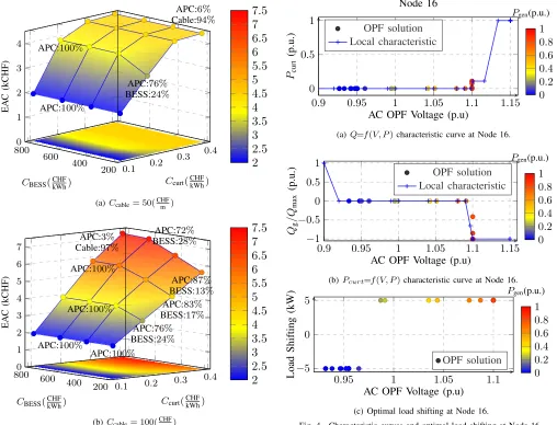
Under the assumption of a fully controllable grid and a perfect communication infrastructure, the DSO would be able to continuously update the setpoints of all units by running OPF calculations with updated measurements of the PV and load injections. However, most of the current distribution grids do not have such advanced communication and control capabilities (yet). Thus, in this section we derive a decen-tralised control scheme (based only on local measurements) that closely approaches the OPF response. Following the methodology of [11], we use the optimal DER setpoints from the OPF-based control of (27), applied to the worst summer day to obtain the Q=f(V, P) and Pcurt=f(V, P)

characteristic curves for all nodes. Figures 4(a) and 4(b) show the corresponding curves for a PV unit and Fig. 4(c) shows the optimal shifting of a flexible load, all connected to Node 16. Simulating the above system with different PV injection and load conditions can allow us to quantify the benefits of using the optimised decentralised control scheme over existing local schemes (as defined by current grid codes). Thus, we compare

0.9 0.95 1 1.05 1.1 1.15 0

0.5 1

AC OPF Voltage (p.u) Pcurt

(p.u.)

Node 16

0 0.2 0.4 0.6 0.8 1

Pgen(p.u.)

OPF solution Local characteristic

(a)Q=f(V, P)characteristic curve at Node 16.

0.9 0.95 1 1.05 1.1 1.15

−1

−0.5 0 0.5 1

AC OPF Voltage (p.u) Qg

/Q

max

(p.u.)

0 0.2 0.4 0.6 0.8 1

Pgen(p.u.)

OPF solution Local characteristic

(b)Pcurt=f(V, P)characteristic curve at Node 16.

0.95 1 1.05 1.1

−5 0 5

AC OPF Voltage (p.u)

Load

Shifting

(kW)

0 0.2 0.4 0.6 0.8 1

Pgen(p.u.)

OPF solution

(c) Optimal load shifting at Node 16.

Fig. 4. Characteristic curves and optimal load shifting at Node 16.

the performance of the following methods

• No control: This case corresponds to simple AC PF for each time step. The PVs are operated having a power factor of one (i.e., without reactive control);

• OPF-based control: A centralised approach is assumed here, where the DERs receive the optimal operational set-points from the OPF solution.

• Default local control: In this case, the PVs behave according to the characteristic curve of the German grid-codes [13]. As soon as they inject more than half of their maximum power, they have to adjust their power factor. • Optimised local control: Finally, in this case each inverter is equipped with different characteristic curves according to [11], and the flexible loads according to Algorithm 1 withVlow

thr = 1.08 p.u. andV up

thr = 0.94p.u., considering

the 2 worst upper / lower optimal setpoints of Fig. 4(c). In the following results, we simulate the grid behavior according to all methods for 30 summer days, i.e. the PV injection and load scaling factors are taken from June.

0 100 200 300 400 500 600 700 0.9

1 1.1

Time (h)

V

oltage

(p.u.)

No control OPF VDE rules Local control Upper limit

Fig. 5. Voltage evolution according to all methods at Node 16.

0 100 200 300 400 500 600 700 0

50 100

Time (h)

V

oltage

(p.u.)

No control OPF VDE rules Local control Upper limit

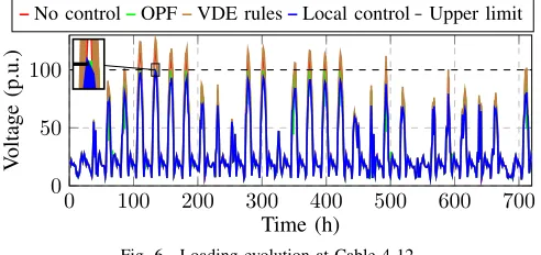
Fig. 6. Loading evolution at Cable 4-12.

leads to frequent voltage limit violations when the difference of PV injection and load is large. On the contrary, both the OPF-based and the optimised local control satisfy the voltage security constraints. Figure 6 shows the loading of the problematic cable 4–12 over the whole month. In this case, the current VDE rules show worse results than without any control due to the increased need for reactive power at Node 12. Both the OPF–based and the proposed local control satisfy the constraint. The first achieves this with the least possible cost, while the latter shows reduced maximum loading due to higher APC (and cost). Finally, Fig. 7 compares the load shifting of the OPF–based against the optimized local control over a period of 2 days. It can be seen that the first makes more frequent use of the flexibility offered by the load, as it is not triggered exclusively by the local voltage values. The optimized local control initiates load shifting mostly at noon hours in order to reduce the local voltage, and once the voltage is within acceptable limits, compensates for the earlier load increase.

V. CONCLUSION

DSOs have nowadays a variety of tools in their disposal to face the planning and operational challenges of the future. These include both conventional expansion decisions as well as active measures. This paper presents a decision-making tool to assist DSOs decide on their planning and operation deci-sions. By co-optimizing the planning and the operation stages, DSOs can assess the trade-offs among the different alternatives and find the optimal balance between hardware-based grid extensions and active grid management. The decision process is formulated as a mixed integer linear problem (MILP), using a tractable iterative AC OPF problem. A sensitivity analysis was performed, varying the most important costs. It demonstrates that the optimal solution is case-dependent and there is no “one-size-fits-all” solution.

80 90 100 110 120

−5 0 5

Time (h) Pshift

(

t

)

(kW)

OPF solution Local control

Fig. 7. Load shifting at Node 16.

Finally, in the transitional phase where extensive communi-cation and control infrastructure is not available in real-time operation, an optimised local control scheme is also presented, tuned by off-line calculations, to provide a near-optimal be-haviour for flexible loads. Results for a summer month show that it is slightly more conservative than the OPF-based control and does not lead to security constraint violations.

REFERENCES

[1] Working Group C6.19, “Planning and Optimization Methods for Active Distribution Systems Working Group C6.19,” Cigre, Tech. Rep. Aug., 2014.

[2] Smart Planning Project WP 2.5, “Planning practices of electrical distri-bution grids.”

[3] P. Paiva, H. Khodr, J. Dominguez-Navarro, J. Yusta, and A. Ur-daneta, “Integral planning of primary-secondary distribution systems using mixed integer linear programming,”IEEE Transactions on Power Systems, vol. 20, no. 2, pp. 1134–1143, 2005.

[4] S. Mohtashami, D. Pudjianto, and G. Strbac, “Strategic Distribution Network Planning With Smart Grid Technologies,”IEEE Transactions on Smart Grid, vol. PP, no. 99, p. 1, 2016.

[5] E. Naderi, H. Seifi, and M. S. Sepasian, “A dynamic approach for distribution system planning considering distributed generation,”IEEE Transactions on Power Delivery, vol. 27, no. 3, pp. 1313–1322, 2012. [6] C. K. Gan, P. Mancarella, D. Pudjianto, and G. Strbac, “Statistical

appraisal of economic design strategies of LV distribution networks,” Electric Power Systems Research, vol. 81, no. 7, pp. 1363–1372, 2011. [7] F. Pilo, G. Celli, E. Ghiani, and G. Soma, “New electricity distribution network planning approaches for integrating renewable,”Wiley Interdis-ciplinary Reviews: Energy and Environment, vol. 2, no. 2, pp. 140–157, 3 2013.

[8] P. S. Georgilakis and N. D. Hatziargyriou, “A review of power distribu-tion planning in the modern power systems era: Models, methods and future research,”Electric Power Systems Research, vol. 121, pp. 89–100, 2015.

[9] P. Fortenbacher, M. Zellner, and G. Andersson, “Optimal Sizing and Placement of Distributed Storage in Low Voltage Networks,” in19th Power Systems Computation Conference 2016, Genoa, Italy, 2016. [10] S. Karagiannopoulos, P. Aristidou, A. Ulbig, S. Koch, and G. Hug,

“Op-timal planning of distribution grids considering active power curtailment and reactive power control,”IEEE Power and Energy Society General Meeting, 2016.

[11] S. Karagiannopoulos, P. Aristidou, and G. Hug, “Hybrid approach for planning and operating active distribution grids,”IET Generation, Transmission & Distribution, vol. 11, no. 3, pp. 685–695, 2017. [12] P. Fortenbacher, A. Ulbig, S. Koch, and G. Andersson, “Grid-constrained

optimal predictive power dispatch in large multi-level power systems with renewable energy sources, and storage devices,” in IEEE PES Innovative Smart Grid Technologies, Europe, Oct. 2014, pp. 1–6. [13] VDE-AR-N 4105, “Power generation systems connected to the LV

distribution network.” FNN, Tech. Rep., 2011.