Hadoop neural network for parallel and distributed feature selection

This is a repository copy of

Hadoop neural network for parallel and distributed feature

selection

.

White Rose Research Online URL for this paper:

http://eprints.whiterose.ac.uk/100474/

Version: Published Version

Article:

Hodge, Victoria Jane orcid.org/0000-0002-2469-0224, O'Keefe, Simon

orcid.org/0000-0001-5957-2474 and Austin, Jim orcid.org/0000-0001-5762-8614 (2016)

Hadoop neural network for parallel and distributed feature selection. Neural Networks.

24–35. ISSN 0893-6080

https://doi.org/10.1016/j.neunet.2015.08.011

[email protected]

https://eprints.whiterose.ac.uk/

Reuse

This article is distributed under the terms of the Creative Commons Attribution (CC BY) licence. This licence

allows you to distribute, remix, tweak, and build upon the work, even commercially, as long as you credit the

authors for the original work. More information and the full terms of the licence here:

https://creativecommons.org/licenses/

Takedown

If you consider content in White Rose Research Online to be in breach of UK law, please notify us by

Contents lists available atScienceDirect

Neural Networks

journal homepage:www.elsevier.com/locate/neunet

2016 Special Issue

Hadoop neural network for parallel and distributed feature selection

Victoria J. Hodge

∗

_{, Simon O’Keefe, Jim Austin}

Advanced Computer Architecture Group, Department of Computer Science, University of York, York, YO10 5GH, UK

a r t i c l e i n f o

Article history:

Available online 5 September 2015

Keywords:

Hadoop MapReduce Distributed Parallel Feature selection Binary neural network

a b s t r a c t

In this paper, we introduce a theoretical basis for a Hadoop-based neural network for parallel and distributed feature selection in Big Data sets. It is underpinned by an associative memory (binary) neural network which is highly amenable to parallel and distributed processing and fits with the Hadoop paradigm. There are many feature selectors described in the literature which all have various strengths and weaknesses. We present the implementation details of five feature selection algorithms constructed using our artificial neural network framework embedded in Hadoop YARN. Hadoop allows parallel and distributed processing. Each feature selector can be divided into subtasks and the subtasks can then be processed in parallel. Multiple feature selectors can also be processed simultaneously (in parallel) allowing multiple feature selectors to be compared. We identify commonalities among the five features selectors. All can be processed in the framework using a single representation and the overall processing can also be greatly reduced by only processing the common aspects of the feature selectors once and propagating these aspects across all five feature selectors as necessary. This allows the best feature selector and the actual features to select to be identified for large and high dimensional data sets through exploiting the efficiency and flexibility of embedding the binary associative-memory neural network in Hadoop.

©2015 The Authors. Published by Elsevier Ltd. This is an open access article under the CC BY license (http://creativecommons.org/licenses/by/4.0/)

1. Introduction

The meaning of ‘‘big’’ with respect to data is specific to each application domain and dependent on the computational resources available. Here we define ‘‘Big Data’’ as large, dynamic collections of data that cannot be processed using traditional techniques, a definition adapted from (Franks,2012;Zikopoulos & Eaton, 2011). Today, data is generated continually by an increasing range of processes and in ever increasing quantities driven by Big Data mechanisms such as cloud computing and on-line services. Business and scientific data from many fields, such as finance, astronomy, bioinformatics and physics, are often measured in terabytes (1012bytes). Big Data is characterised by its complexity, variety, speed of processing and volume (Laney, 2001). It is increasingly clear that exploiting the power of these data is essential for information mining. These data often contain too much noise (Liu, Motoda, Setiono, & Zhao, 2010) for accurate classification (Dash & Liu, 1997;Han & Kamber, 2006), prediction

∗_{Correspondence to: Department of Computer Science, University of York,}

Deramore Lane, York, YO10 5GH, UK. Tel.: +44 01904 325637; fax: +44 01904 325599.

E-mail addresses:[email protected](V.J. Hodge),

[email protected](S. O’Keefe),[email protected](J. Austin).

(Dash & Liu, 1997;Guyon & Elisseeff, 2003) or outlier detection (Hodge, 2011). Thus, only some of the features (dimensions) are related to the target concept (classification label or predicted value). Also, if there are too many data features then the data points become sparse. If data is too sparse then distance measures such as the popular Euclidean distance and the concept of nearest neighbours become less applicable (Ertöz, Steinbach, & Kumar, 2003). Many machine learning algorithms are adversely affected by this noise and these superfluous features in terms of both their accuracy and their ability to generalise. Consequently, the data must be pre-processed by the classification or prediction algorithm itself or by a separate feature selection algorithm to prune these superfluous features (Kohavi & John, 1997;Witten & Frank, 2000). The benefits of feature selection include: reducing the data size when superfluous features are discarded, improving the classification/prediction accuracy of the underlying algorithm where the algorithm is adversely affected by noise, producing a more compact and easily understood data representation and reducing the execution time of the underlying algorithm due to the smaller data size. Reducing the execution time is extremely important for Big Data, which has a high computational resource demand on memory and CPU time.

In this paper, we focus on feature selection in vast data sets for parallel and distributed classification systems. We aim to remove

http://dx.doi.org/10.1016/j.neunet.2015.08.011

V.J. Hodge et al. / Neural Networks 78 (2016) 24–35

noise and reduce redundancy to improve classification accuracy. There is a wide variety of techniques proposed in the machine learning literature for feature selection including Correlation-based Feature Selection (Hall, 1998), Principal Component Analysis (PCA) (Jolliffe, 2002), Information Gain (Quinlan, 1986), Gain Ratio (Quinlan, 1992), Mutual Information Selection (Wettscherek, 1994), Chi-square Selection (Liu & Setiono, 1995), Probabilistic Las Vegas Selection (Liu & Setiono, 1996) and Support Vector Machine Feature Elimination (Guyon, Weston, Barnhill, & Vapnik, 2002). Feature selectors produce feature scores. Some feature selectors also select the best set of features to use while others just rank the features with the scores. For these feature rankers, the best set of features must then be chosen by the user, for example, using greedy search (Witten & Frank, 2000).

It is often not clear to the user which feature selector to use for their data and application. In their analysis of feature selection, Guyon and Elisseeff (2003) recommend evaluating a variety of feature selectors before deciding the best for their problem. Therefore, we propose that users exploit our framework to run a variety of feature selectors in parallel and then evaluate the feature sets chosen by each selector using their own specific criteria. Having multiple feature selectors available also provides the opportunity for ensemble feature selection where the results from a range of feature selectors are merged to generate the best set of features to use. Feature selection is a combinatorial problem so needs to be implemented as efficiently as possible particularly on big data sets. We have previously developed a k-NN classification (Hodge & Austin, 2005; Weeks, Hodge, O’Keefe, Austin, & Lees, 2003) and prediction algorithm (Hodge, Krishnan, Austin, & Polak, 2011) using an associative memory (binary) neural network called the Advanced Uncertain Reasoning Architecture (AURA) (Austin, 1995). This multi-faceted k-NN motivated a unified feature selection framework exploiting the speed and storage efficiency of the associative memory neural network. The framework lends itself to parallel and distributed processing across multiple nodes allowing vast data sets to be processed. This could be done by processing the data at the same geographical location using a single machine with multiple processing cores (Weeks, Hodge, & Austin, 2002) or at the same geographical location using multiple compute nodes (Weeks et al., 2002) or even distributed processing of the data at multiple geographical locations.

Data mining tools such as Weka (Witten & Frank, 2000), Matlab,Rand SPSS provide feature selection algorithms for data mining and analytics. However, these products are designed for small scale data analysis. Researchers have parallelised individual feature selection algorithms using MapReduce/Hadoop (Chu et al., 2007; Reggiani, 2013; Singh, Kubica, Larsen, & Sorokina, 2009; Sun, 2014). Data mining libraries such as Mahout (https:// mahout.apache.org) and MLib (https://spark.apache.org/mllib/) and data mining frameworks such as Radoop (https://rapidminer. com/products/radoop/) include a large number of data mining algorithms including feature selectors. However, they do not explicitly tackle processing reuse with a view to multi-user and multi-task resource allocation. Zhang, Kumar, and Ré (2014) developed a database systems framework for optimised feature selection providing a range of algorithms. They observed that there are reuse opportunities that could yield orders of magnitude performance improvements on feature selection workloads as we will also demonstrate here using AURA in an Apache Hadoop (https://hadoop.apache.org/) framework.

The main contributions of this paper are:

•

To extend the AURA framework to parallel and distributed processing of vast data sets in Apache Hadoop,

•

To describe five feature selectors in terms of the AURA frame-work. Two of the feature selectors have been implemented in AURA but not using Hadoop (Hodge, Jackson, & Austin, 2012; Hodge, O’Keefe, & Austin, 2006) and the other three have not been implemented in AURA before,

•

To theoretically analyse the resulting framework to show how the five feature selectors have common requirements to enable reuse.

•

To theoretically analyse the resulting framework to show how we reduce the number of computations. The larger the data set then the more important this reduction becomes.

•

To demonstrate parallel and distributed processing in the framework allowing Big Data to be analysed.

In our AURA framework, the feature selectors all use one com-mon data representation. We only need to process any comcom-mon elements once and can propagate the common elements to all feature selectors that require them. Thus, we can rapidly and ef-ficiently determine the best feature selector and the best set of features to use for each data set under investigation. In Section2, we discuss AURA and related neural networks and how to store and retrieve data from AURA, Section3demonstrates how to im-plement five feature selection algorithms in the AURA unified framework and Section4describes parallel and distributed feature selection using AURA. We than analyse the unified framework in Section5to identify common aspects of the five feature selectors and how they can be implemented in the unified framework in the most efficient way. Section6details the overall conclusions from our implementations and analyses.

2. Binary neural networks

AURA (Austin, 1995) is a hetero-associative memory neural network (Palm, 2013). An associative memory is addressable through its contents and a hetero-associative memory stores associations between input and output vectors where the vectors are different (Palm, 2013). AURA uses binary Correlation Matrix Memories (CMMs): binary hetero-associative matrices that store and retrieve patterns using matrix calculus. They are non-recursive and fully connected. Input vectors (stimuli) address the CMM rows and output vectors address the CMM columns. Binary neural networks have a number of advantages compared to standard neural networks including rapid one-pass training, high levels of data compression, computational simplicity, network transparency, a partial match capability and a scalable architecture that can be easily mapped onto high performance computing platforms including parallel and distributed platforms (Weeks et al., 2002). AURA is implemented as a C++ software library.

Previous parallel and distributed applications of AURA have included distributed text retrieval (Weeks et al., 2002), distributed time-series signal searching (Fletcher, Jackson, Jessop, Liang, & Austin, 2006) and condition monitoring (Austin, Brewer, Jackson, & Hodge, 2010). This new development will augment these existing techniques and is aimed at these same domains. It will couple feature selection, classification and prediction with the speed and storage efficiency of a binary neural network allowing parallel and distributed data mining. This makes AURA ideal to use as the basis of an efficient distributed machine learning framework. A more formal definition of AURA, its components and methods now follows.

2.1. AURA

[image:4.595.359.492.60.230.2]

V.J. Hodge et al. / Neural Networks 78 (2016) 24–35

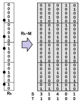
Fig. 1. Showing a CMM learning input vectorInassociated with output vectorOn

on the left. The CMM on the right shows the CMM after five associationsIjOTj. Each

column of the CMM represents a record. Each row represents a feature value for qualitative features or a quantisation of feature values for quantitative features and each set of rows (shown by the horizontal lines) represents the set of values or set of quantisations for a particular feature.

rule (Palm, 2013).

M

=



IjOTj where

∨

is logical OR

.

(1)

Training (construction of a CMM) is a single epoch process with one training step for each input–output association (eachIjOTj in

Eq. (1)) which equates to one step for each record j in the data set. Thus, the trained CMMM represents

{

(

I1

×

OT1

), (

I2

×

OT

2

), . . . (

In

×

OTn

)

}

superimposed using bitwise or. IjOTj is an

estimate of the weight matrixW

(

j

)

of the synaptic connections of the neural network as a linear associator with binary weights.W

(

j

)

forms a mapping representing the association described by thejth input/output pair of vectors. As a consequence of using unipolar elements {0,1} throughout, the value at each matrix componentwij

means the existence of an association between elementsiandj. The trained CMMMis then effectively an encoding (correlation) of theNweight matricesWfor allNrecords in the data set. Individual weights within the weight matrix update using a generalisation of Hebbian learning (Hebb, 1949) where the state for each synapse (matrix element) is binary valued. Every synapse can update its weight independently using a local learning rule (Palm, 2013). Local learning is biologically plausible and computationally simple allowing parallel and rapid execution. The learning process is illustrated inFig. 1.

For feature selection, the data are stored in the CMM which forms an index of all features in all records. During training, the input vectors Ij represent the feature and class values and are

associated with a unique output vectorOjrepresenting a record.

Fig. 1shows a trained CMM. In this paper, we set only one bit in the vectorOjindicating the location of the record in the data set, the

first record has the first bit set, the second record has the second bit set etc. Using a single set bit makes the length ofOjpotentially

large. However, exploiting a compact list representation (Hodge & Austin, 2001) (more detail is provided in Section4.3.1) means we can compress the storage representation.

2.2. Data

The AURA feature selector, classifier and predictor framework can handle qualitative features (symbolic and discrete numeric) and quantitative features (continuous numeric).

The raw data sets need pre-processing to allow them to be used in the binary AURA framework. Qualitative features are enumer-ated and each separate token maps onto an integer (Token

→

Integer) which identifies the bit to set within the vector. For ex-ample, a SEX_TYPE feature would map as (F

→

0) and (M

→

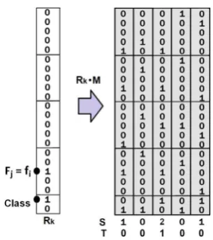
1).

Fig. 2. Showing a CMM recall. Applying the recall input vectorRkto the CMMM

retrieves a summed integer vectorSwith the match score for each CMM column.S

is then thresholded to retrieve the matches. The threshold here is either Willshaw with value 3 retrieving all columns that sum to 3 or more or L-Max with value 2 to retrieve the 2 highest scoring columns.

Any quantitative features are quantised (mapped to discrete bins) (Hodge & Austin, 2012). Each individual bin maps onto an integer which identifies the bit to set in the input vector. Next, we describe the simple equi-width quantisation. We note that the Correlation-Based Feature Selector described in Section3.2uses a different quantisation technique to determine the bin boundaries. However, once the boundaries are determined, the mapping to CMM rows is the same as described here.

To quantise quantitative features, a range of input values for featureFf map onto each bin. Each bin maps to a unique integer

as in Eq.(2)to index the correct location for the feature inIj. In

this paper, the range of feature values mapping to each bin is equal to subdivide the feature range intobequi-width bins across each feature.

R_fi

→

bins_fk

→

Integer_f

k

+

offset



F_f



whereFf

∈

F

,

fi is a value ofFfandcardinality



Integer_fk



≡

cardinality

(

binsfk

).

(2)

In Eq.(2),offset

(

Ff

)

is a cumulative integer offset within the

binary vector for each featureFf,

→

is a many-to-one mapping and

→

is a one-to-one mapping. The offset for the next featureFf+1is

given byoffset

(

Ff+1

)

=

offset

(

Ff

)

+

nBins

(

Ff

)

wherenBins

(

Ff

)

is

the number of bins for featureF_f.

For each record in the data set. For each feature.

Calculate bin for feature value. Set bit in vector as in Eq.(2).

2.3. AURA recall

To recall the matches for a query (input) record, we firstly produce a recall input vectorRk by quantising the target values

for each feature to identify the bins (CMM rows) to activate as in Eq.(3). During recall, the presentation of recall input vectorRk

elicits the recall of output vectorOk as vectorRk contains all of

the addressing information necessary to access and retrieve vector

O_k. Recall is effectively the dot product of the recall input vectorR_k

and CMMM, as in Eq.(3)andFig. 2.

ST

=

R_kT

·

M

.

(3)

[image:4.595.49.269.63.205.2]

[image:5.595.91.244.59.231.2]

V.J. Hodge et al. / Neural Networks 78 (2016) 24–35

Fig. 3. Diagram showing the feature value row and the class values row excited to

determine co-occurrences (C=c Fj=fi).

output vector multiplied by a weight based on the dot product of the input vector with itself. If the recall inputRk is not from

the original training set, then the system will recall the outputOk

associated with the closest stored input toRk, based on the dot

product between the test and training inputs.

Matching is a combinatorial problem but can be achieved in a single pass in AURA. AURA can also exploit the advantages of sparse vectors (Palm, 2013) during recall by only activating regions of interest. If the input vectorRkhas 1000 bits indexing 1000 CMM

rows then only the rows addressed by a set bit in the input vector need be examined (as shown inFigs. 2and3). For a 10 bit set vector then only 10 of the 1000 rows are activated. The input pattern

R_k would be said to have a saturation of (10

/

1000

=

0

.

01). The total amount of data that needs to be examined is reduced by a factor that is dependent on this saturation providing that the data is spread reasonably evenly between the rows and the CMM is implemented effectively. Using smart encoding schemes can bring the performance improvement resulting from very low saturation input patterns to over 100-fold (Weeks et al., 2002).

The AURA technique thresholds the summed output S to produce a binary output vectorTas given in Eq.(4).

Tj

=



1 ifSj

≥

θ

0 otherwise

.

(4)

For exact match, we use the Willshaw threshold (Willshaw, Buneman, & Longuet-Higgins, 1969) to set

θ

. This sets a bit in the thresholded output vector for every location in the summed output vector that has a value higher than or equal to

θ

. The value of

θ

varies according to the task. If there are ten features in the data and we want to find all stored records that match the ten feature values of the input vector then we set

θ

to 10. Thus, for full match

θ

=

b1, whereb1is set to the number of set bits in the input vector. For partial matching, we use the L-Max threshold (Casasent & Telfer, 1992). L-Max thresholding essentially retrievesat least L top matches. Our AURA software library automatically sets

θ

to the highest integer value that will retrieve at leastLmatches.

Feature selection described in Section3 requires both exact matching using Willshaw thresholding and partial matching using L-Max thresholding.

3. Feature selection

There are two fundamental approaches to feature selection (Kohavi & John, 1997;Witten & Frank, 2000): (1) filters select the optimal set of features independently of the classifier/predictor algorithm while (2) wrappers select features which optimise

classification/prediction using the algorithm. We examine the mapping of five filter approaches to the binary AURA architecture. Filter approaches are more flexible than wrapper approaches as they are not directly coupled to the algorithm and are thus applicable to a wide variety of classification and prediction algorithms. Our method exploits the high speed and efficiency of the AURA techniques as feature selection is a combinatorial problem.

We examine a mutual information approachMutual Informa-tion Feature SelecInforma-tion (MI)detailed in Section3.1that analyses features on an individual basis, a correlation-based multivariate filter approachCorrelation-based Feature Subset Selection (CFS) detailed in Section3.2that examines greedily selected subsets of features, a revised Information Gain approachGain Ratio (GR) de-tailed in Section3.3, a feature dependence approachChi-Square Feature selection(CS)detailed in Section3.4which is univariate, and a univariate feature relevance approachOdds Ratio (OR) de-tailed in Section3.5.

Univariate filter approaches such as MI, CS or OR are quicker than multivariate filters as they do not need to evaluate all com-binations of subsets of features. The advantage of a multivariate filter compared to a univariate filter lies in the fact that a univari-ate approach does not account for interactions between features. Multivariate techniques evaluate the worth of feature subsets by considering both the individual predictive ability of each feature and the degree of redundancy between the features in the set.

All five feature selection algorithms have their relative strengths. We refer the reader toForman(2003) andVarela, Mar-tins, Aguiar, and Figueiredo (2013) for accuracy evaluations of these feature selectors. These papers show that the best feature selector varies with data and application. Using the CFS attribute selector,Hall and Smith(1998) found significant improvement in classification accuracy of k-NN on five of the 12 data sets they eval-uated but a significant degradation in accuracy on two data sets. Hence, different feature selectors are required for different data sets and applications.

We note that the CFS as implemented by Hall (1998) uses an entropy-based quantisation whereas we have used equi-width quantisation for the other feature selectors (MI, GR, CS and OR). We plan to investigate unifying the quantisation as a next step. For the purpose of our analysis in Section5, we assume that all feature selectors are using identical quantisation. We assume that all records are to be used during feature selection.

3.1. Mutual information feature selection

Wettscherek (1994) described a mutual information feature selection algorithm. The mutual information between two features is ‘‘the reduction in uncertainty concerning the possible values of one feature that is obtained when the value of the other feature is determined’’ (Wettscherek, 1994). MI is defined by Eq.(5):

MI



F_j

,

C



=

b(Fj)



i=1

nClass



c=1

p

(

C

=

c



F_j

=

f_i

)

·

log₂



p

(

C

=

c



Fj

=

fi

)

p

(

C

=

c

)

·

p

(

Fj

=

fi

)



.

(5)

To calculatep

(

C

=

c



Fj

=

fi

)

, we use AURA to calculate

n(BVfi∧BVc)

N .

AURA excites the row in the CMM corresponding to feature value fi of feature Fj and the row in the CMM corresponding

V.J. Hodge et al. / Neural Networks 78 (2016) 24–35

p

(

C

=

c

)

is the count of the number of set bitsn

(

BVc

)

in the binary vector (CMM row) forcandp

(

Fj

=

fi

)

is the count of the number of set bitsn

(

BVf_i

)

in the binary vector (CMM row) forfias used by

GR.

The MI calculated using AURA for qualitative features is given by Eq.(6)whereNis the number of records in the data set,rows

(

Fj

)

is the number of CMM rows for featureFjandnClassis the number

of classes:

MI



Fj

,

C



=

rows(Fj)



i=1

nClass



c=1

n

(

BV fi

∧

BVc

)

N

·

log₂



_{n(BV fi∧BVc)}

N n(BV fi)

N

·

n(BVc)

N



.

(6)

We can follow the same process for real/discrete ordered numeric features in AURA. In this case, the mutual information is given by Eq.(7):

MI



Fj

,

C



=

bins(Fj)



i=1

nClass



c=1

n

(

BV bi

∧

BVc

)

N

·

log₂



_{n(BV b}

i∧BVc)

N n(BV bi)

N

·

n(BVc)

N



(7)

wherebins

(

Fj

)

is the number of bins (effectively the number of

rows) in the CMM for featureFjandBVbiis the CMM row for the

bin mapped to by feature valuefi.

The MI feature selector assumes independence of features and scores each feature separately so it is the user’s prerogative to determine the number of features to select. The major drawback of the MI feature selector along with similar information theoretic approaches, for example Information Gain, is that they are biased towards features with the largest number of distinct values as this splits the training records into nearly pure classes. Thus, a feature with a distinct value for each record has a maximal information score. The CFS and GR feature selectors make adaptations of information theoretic approaches to prevent this biasing.

3.2. Correlation-based feature subset selection

Hall (1998) proposed the Correlation-based Feature Subset Selection (CFS). It measures the strength of the correlation between pairs of features. CFS favours feature subsets that contain features that are highly correlated to the class but uncorrelated to each other to minimise feature redundancy. CFS is thus based on information theory measured using Information Gain. Hall and Smith (1997) used a modified Information Gain measure, Symmetrical Uncertainty, (SU) given in Eq. (8) to prevent bias towards features with many distinct values (Section 3.1). SU

estimates the correlation between features by normalising the value in the range [0, 1]. Two features are completely independent ifSU

=

0and completely dependent ifSU

=

1.

SU



Fj

,

Gl



=

2

.

0

·



Ent



Fj



−

Ent



Fj

|

Gl



Ent



F_j



+

Ent

(

G_l

)



(8)

where the entropy of a featureFjfor all feature valuesfiis given as

Eq.(9):

Ent



Fj



= −

n(Fj)



i=1

p

(

fi

)

log2

(

p

(

fi

))

(9)

and the entropy of featureFjafter observing values of featureGlis

given as Eq.(10):

Ent



Fj

|

Gl



= −

n(Gl)



k=1

p

(

gk

)

n(Fj)



i=1

p

(

fi

|

gk

)

log2

(

p

(

fi

|

gk

)).

(10)

Any quantitative features are discretised using Fayyad and Irani’s entropy quantisation (Fayyad & Irani, 1993). The bin bound-aries are determined using Information Gain and these quantisa-tion bins map the data into the AURA CMM as previously.

CFS has many similarities to MI when calculating the values in Eqs.(8)–(10)and through using the same CMM (Fig. 3) as noted below.

In the AURA CFS, for each pair of features (Fj

,

Gl) to be examined,

the CMM is used to calculateEnt

(

F_j

),

Ent

(

G_l

)

andEnt

(

F_j

|

G_l

)

from Eqs.(8)–(10). There are three parts to the calculation.

1. Ent

(

Fj

)

requires the count of data records for the particular

valuefiof featureFjwhich isn

(

BVfi

)

in Eq.(6)for qualitative

and class features and n

(

BVbi

)

in Eq. (7) for quantitative

features. AURA excites the row in the CMM corresponding to feature valuefiof featureFj. This row is a binary vector (BV)

and is represented byBVf_i. A count of bits set on the row gives

n

(

BVf_i

)

from Eq.(6)and is achieved by thresholding the output vectorSkfrom Eq.(4)at Willshaw value 1.

2. Similarly,Ent

(

Gl

)

counts the number of records where feature

Glhas valuegk.

3. Ent

(

Fj

|

Gl

)

requires the number of co-occurrences of a

partic-ular valuefiof featureFjwith a particular valuegk of feature

Gln

(

BVfi

∧

BVgk

)

for qualitative features andn

(

BVbi

∧

BVbk

)

for quantitative features and between a feature and the class

n

(

BVf_i

∧

BVc

)

andn

(

BVbi

∧

BVc

)

for qualitative and

quanti-tative features respectively. If both the feature value row and the class values row are excited then the summed output vec-tor will have a two in the column of every record with a co-occurrence offiwithcjas shown inFig. 3. By thresholding the

summed output vector at a threshold of two, we can find all co-occurrences. We represent this number of bits set in the vector byn

(

BVf_i

∧

BVc

)

which is a count of the set bits whenBVcis logicallyanded withBVf_i.

CFS determines the feature subsets to evaluate using forward search. Forward search works by greedily adding features to a subset of selected features until some termination condition is met whereby adding new features to the subset does not increase the discriminatory power of the subset above a pre-specified threshold value. The major drawback of CFS is that it cannot handle strongly interacting features (Hall & Holmes, 2003).

3.3. Gain ratio feature selection

Gain Ratio (GR) (Quinlan, 1992) is a new feature selector for the AURA framework. GR is a modified Information Gain technique and is used in the popular machine learning decision tree classifier C4.5 (Quinlan, 1992). Information Gain is given in Eq.(11)for feature

Fj and the classC. CFS (Section3.2) modifies Information Gain

to prevent biasing towards features with the most values. GR is an alternative adaptation which considers the number of splits (number of values) of each feature when calculating the score for each feature using normalisation.

Gain



Fj

,

C



=

Ent



Fj



−

Ent

(

Fj

|

C

)

(11)

whereEnt

(

Fj

)

is defined in Eq.(9)andEnt

(

Fj

|

C

)

is defined by

Eq.(10). Then Gain Ratio is defined as Eq.(12):

GainRatio



Fj

,

C



=

Gain

(

Fj

,

C

)

IntrinsicValue

(

Fj

)

(12)

whereIntrinsicValueis given by Eq.(13):

IntrinsicValue



F_j



=

V



p=1

Sp

Nlog2



Sp

N



V.J. Hodge et al. / Neural Networks 78 (2016) 24–35

and V is the number of feature values

(

n

(

Fj

))

for qualitative

features and number of quantisation binsn

(

bi

)

for quantitative

features and Sp is a subset of the records that have Fj

=

fi

for qualitative features or map to the quantisation binbin

(

fi

)

for

quantitative features.

To implement GR using AURA, we train the CMM as described in Section2.1We can then calculateEnt

(

Fj

)

andEnt

(

Fj

|

C

)

as per the

CFS feature selector described in Section3.2to allow us to calculate

Gain

(

Fj

,

C

)

. To calculateIntrinsicValue

(

Fj

)

we need to calculate

the number of records that have particular feature values. This is achieved by counting the number of set bitsn

(

BVf_i

)

in the binary vector (CMM row) forfifor qualitative features orn

(

BVbi

)

in the

binary vector for the quantisation binb_ifor quantitative features. We can store counts for the various feature values and classes as we proceed so there is no need to calculate any count more than once.

The main disadvantage of GR is that it tends to favour features with low Intrinsic Value rather than high gain by overcompensat-ing towards a feature just because its intrinsic information is very low.

3.4. Chi-square algorithm

We now demonstrate how to implement a second new feature selector in the AURA framework. The Chi-Square (CS) (Liu & Setiono, 1995) algorithm is a feature ranker like MI, OR and GR rather than a feature selector; it scores the features but it is the user’s prerogative to select which features to use. CS assesses the independence between a feature

(

Fj

)

and a class (C) and is sensitive

to feature interactions with the class. Features are independent if CS is close to zero.Forman(2003) andYang and Pedersen(1997) conducted evaluations of filter feature selectors and found that CS is among the most effective methods of feature selection for classification.

Chi-Square is defined as Eq.(14):

χ

2



Fj

,

C



=

b(Fj)



i=1

nClass



c=1

N

∗

(

wz

−

yx

)

2

(

w

+

y

)

∗

(

x

+

z

)

∗

(

w

+

x

)

∗

(

y

+

z

)

(14)

where b

(

F_j

)

is the number of bins (CMM rows) representing feature Fj, nClass is the number of classes, w is the number

of times fi and c co-occur, x is the number of times fi occurs

withoutc

,

yis the number of timescoccurs withoutfi

,

zis the

number of times neithercnorfioccur. Thus, CS is predicated on

counting occurrences and co-occurrences and, hence, has many commonalities with MI, CFS and GR.

•

Fig. 3shows how to produce a binary output vector (BVf_i

∧

BVc) for qualitative features or (BVbi

∧

BVc) for quantitative features

listing the co-occurrences of a feature value and a class value. It is then simply a case of counting the number of set bits (1s) in the thresholded binary vectorTinFig. 3to countw.

•

To countxfor qualitative features, we logically subtract (BVf_i

∧

BVc) from the binary vector (BVf_i) to produce a binary vector and count the set bits in the resulting vector. For quantitative features, we subtract (BVbi

∧

BVc) from (BVbi) and count the

set bits in the resulting binary vector.

•

To county for qualitative features, we can logically subtract (BVf_i

∧

BVc) from (BVc) and count the set bits and likewise for quantitative features we can subtract (BVbi

∧

BVc) fromBVc

and count the set bits.

•

If we logicallyor (BVf_i) with (BVc), we get a binary vector representing

(

Fj

=

fi

)

∨

(

C

=

c

)

for qualitative features. For

quantitative features, we can logicallyor(BVbi) with (BVc) to

produce

(

Fj

=

bin

(

fi

))

∨

(

C

=

c

)

. If we then logically invert

this new binary vector, we retrieve a binary vector representing

zand it is simply a case of counting the set bits to get the count forz.

As with MI and OR, CS is univariate and assesses features on an individual basis selecting the features with the highest scores, namely the features that interact most with the class.

3.5. Odds ratio

The third new feature selector is Odds Ratio (OR) (seeForman, 2003). OR is another feature ranker. Standard OR is a two-class feature ranker although it can be extended to multiple classes. It is often used in text classification tasks as these are often two-class problems. It performs well particularly when used with Naïve Bayes Classifiers. OR reflects relevance as the likelihood (odds) of a feature occurring in the positive class normalised by that of the negative class. OR has many commonalities with MI, CFS and GR but particularly with CS where it requires the same four calculations

w

,x,yandz(defined above in Section3.4). Odds Ratio is defined by Eq.(15):

OR



Fj

,

C



=

b(Fj)



i=1

wz

yx (15)

whereb

(

Fj

)

is the number of bins (CMM rows) representing feature

Fj,wis the number of timesfi andcco-occur,xis the number

of timesfioccurs withoutc,yis the number of timesc occurs

withoutfi,zis the number of times neitherc norfioccur. Thus,

OR is predicated on counting occurrences and co-occurrences. To avoid division by zero the denominator is set to 1 ifyxevaluates to 0.

4. Parallel and distributed AURA

Feature selection is a combinatorial problem so a fast, efficient and scalable platform will allow rapid analysis of large and high dimensional data sets. AURA has demonstrated superior training and recall speed compared to conventional indexing approaches (Hodge & Austin, 2001) such as hashing or inverted file lists which may be used for data indexing. AURA trains 20 times faster than an inverted file list and 16 times faster than a hashing algorithm. It is up to 24 times faster than the inverted file list for recall and up to 14 times faster than the hashing algorithm. AURA k-NN has demonstrated superior speed compared to conventional k-NN (Hodge & Austin, 2005) and does not suffer the limitations of other k-NN optimisations such as the KD-tree which only scales to low dimensionality data sets (McCallum, Nigam, & Ungar, 2000). We showed inHodge et al. (2006) that using AURA speeds up the MI feature selector by over 100 times compared to a standard implementation of MI.

For very large data sets, the data may be processed in parallel on one compute node (such as a multi-core CPU) or across a number of distributed compute nodes. Each compute node in a distributed system can itself perform parallel processing.

4.1. Parallel AURA

In Weeks et al. (2002), we demonstrated a parallel search implementation of AURA. AURA can be subdivided across multiple processor cores within a single machine or spread across multiple connected compute nodes. This parallel processing entails ‘‘striping’’ the CMM across several parallel subsections. The CMM is effectively subdivided vertically across the output vector as shown inFig. 4. In the data, the number of featuresmis usually much less than the number of recordsN,m

≪

N. Therefore, we subdivide the data along the number of recordsN(column stripes) as shown in the leftmost example inFig. 4.

[image:8.595.116.469.61.193.2]

V.J. Hodge et al. / Neural Networks 78 (2016) 24–35

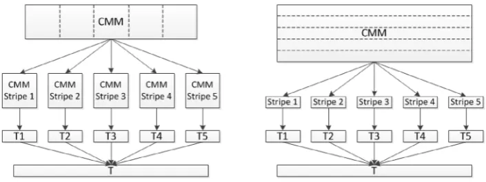
Fig. 4. If a CMM contains large data it can be subdivided (striped) across a number of CMM stripes. In the left hand figure, the CMM is striped vertically (by time) and in the

right hand figure the CMM is striped horizontally (be feature subsets). On the left, each CMM stripe produces a thresholded output vectorTncontaining the topkmatches

(and their respective scores) for that stripe. All{Tn}are aggregated to form a single output vectorTwhich is thresholded to list the top matches overall. On the right, each

stripe outputs a summed output vectorSn. AllSnare summed to produce an overall summed output vector which is thresholded to list the top matches overall.

stripe. Each record is contained within a single stripe. Each separate CMM stripe outputs a thresholded vector from that CMM stripe.

If the number of features is large then it is possible to subdivide the CMMs further. The CMM is divided vertically by the records (column stripes) as before and then the column stripes are subdivided by the input features (row stripes). Subdivision by input features (row stripes) is shown in the rightmost diagram in Fig. 4. Dividing the CMM using the features (row stripes) makes assimilating the results more complex than assimilating the results for column stripes. Each row stripe produces a summed output vector containing column subtotals for those features within the stripe. The column subtotals need to be assimilated from all row stripes that hold data for that column. Thus, we sum these column subtotals to produce a column stripe vectorCholding the overall sum for each column in that stripe. Row striping involves assimilating integer vectors of lengthcwherecis the number of columns for the column subdivision (column stripe).

4.2. Distributed AURA

There are two central challenges for distributed feature selec-tion: firstly, maintaining a distributed data archive so that data does not have to be moved to a central repository and secondly, orchestrating the search process across the distributed data. Dif-ferent data and applications will have difDif-ferent criteria that they wish to optimise. These could be optimising communication over-head, processing speed, memory usage or combinations of these criteria. Hence, there is unlikely to be a single best technique for distribution.

To distribute AURA, we use the striping mechanisms detailed in the previous section. However, rather than spreading the stripes within the cores of a multicore processor, we distribute the stripes across computers within a distributed network. The stripes need to be distributed for maximum efficiency. This can be to maximise processing speed, to minimise memory usage, to minimise communication overhead or a combination of criteria. Distributing the stripes requires an efficient distribution mechanism to underpin the procedure.

Orchestrated search with minimal data movement is provided by the open source software project: Apache Hadoop (Shvachko, Hairong, Radia, & Chansler, 2010). Hadoop operates on the premise that ‘‘moving computation is cheaper than moving data’’ (Borthakur, 2008). Hadoop allows the distributed processing of large data sets across clusters of commodity servers. It provides load balancing, is highly scalable and has a very high degree of fault tolerance. It is able to run on commodity hardware due to its ability to detect and handle failures at the application layer. There are multiple copies of the stored data so, if one server or node is unavailable, its data can

be automatically replicated from a known good copy. If a compute node fails then Hadoop automatically re-balances the work load on the remaining nodes. Hadoop has demonstrated high performance for a wide variety of tasks (Borthakur et al., 2011). It was initially aimed at batch processing tasks so is ideally suited to the task of feature selection where the feature selector is trained with the training data and feature selection is run once on a large batch of test data. Hadoop is currently developing real-time processing capabilities. In this paper, we focus on batch processing and the implementation details of the five feature selectors using AURA with Hadoop.

Hadoop is highly configurable and can be optimised to the user’s specific requirements, for example, optimising to minimise memory overhead, optimising for fastest processing or optimising to reduce communication overhead. Hence, we do not attempt to evaluate Hadoop here. Instead, we focus on describing how to map AURA CMMs to Hadoop to create a feature evaluation framework.

There are two parts of Hadoop that we consider here: YARN which assigns work to the nodes in a cluster and the Hadoop Distributed File System (HDFS) which is a distributed file system spanning all the nodes in the Hadoop cluster with a single namespace.

YARN (Kumar et al., 2013) supersedes MapReduce in Hadoop. YARN is able to run existing MapReduce applications. YARN decouples resource management and scheduling from the data processing. This means that data can continue to be streamed into the system simultaneously with MapReduce batch jobs. YARN has a central resource manager that reconciles Hadoop system resources according to constraints such as queue capacities or user-limits. Node manager agents monitor the processing operations of individual nodes in the cluster. The processing is controlled by an ApplicationMaster which negotiates resources from the central resource manager and works with the node manager agents to execute and monitor the tasks. The actual MapReduce procedure, divides (maps) the processing into separate chunks which are processed in parallel. The outputs of the processing tasks are combined (reduced) to generate a single result. The input and output data for MapReduce can be stored in HDFS on the same compute nodes used for processing the MapReduce jobs. This produces a very high aggregate bandwidth across the cluster. The user’s applications specify the input/output locations and supply map and reduce functions via implementations of appropriate interfaces and/or abstract-classes. The framework takes care of distributing the software/configuration, scheduling tasks, monitoring the tasks and re-executing any failed tasks.

[image:9.595.168.442.57.292.2]

V.J. Hodge et al. / Neural Networks 78 (2016) 24–35

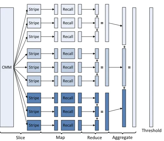
Fig. 5. Figure showing distributed AURA recall in Hadoop. In the figure, there are three distributed compute nodes as shown by the shading with three CMM stripes per node

(3 CPU cores per node and one stripe per core). Thus, the top three stripes are on one compute node spread across three cores. In the map phase, the required input vectors are applied to the CMM stripes and the summed output vector is recalled for each stripe. The summed output vector can be thresholded now or later following aggregation as described in Section4.3.1. During the reduce phase, these output vectors are aggregated at each compute node giving three aggregated vectors. Finally, the three vectors are combined.

moving the data over the network to a single processing node. This local processing architecture of Hadoop has resulted in very good performance (Rutman, 2011) on cheap computer clusters even with relatively slow network connections (such as 1 Gig Ethernet) (Rutman, 2011). Hence, Hadoop is ideal to underpin our distributed processing architecture.

4.3. Hadoop feature selection

Feature selection is a two part procedure. A training phase described in Section 2.1 trains the data into the CMMs. A test phase then applies test data to the trained CMMs and correlates the results to produce feature selections. Each compute node holds a CMM, CMM stripe or set of CMM stripes that stores all local data. During training, CMMs are not immutable as each association in Eq.(1)changes the underlying CMM so Hadoop MapReduce is not a suitable paradigm for CMM training. Hence, the CMMs are trained in a conventional fashion and uploaded to HDFS once trained. If the data stored in a node’s CMM exceed the memory capacity of that node then the CMM is subdivided into stripes as described in Section4.1 and shown in Figs. 4and 5. The set of all CMM stripes at a node stores all data for that node. Every CMM stripe across the distributed system has to be coordinated so that record identifiers (such as timestamps) are matched to allow the CMM sum and threshold. Sum and threshold is column-based and relies on columns representing the same datum. When the results from different CMMs are unified then the columns from the various CMMs need to be aligned. The system is very flexible; we only need to access relevant CMM stripes so we can access subsets of data. The approach is a combination of the striping described above in Section4.1and the CMM distribution described in Section4.2with Hadoop orchestrating the search.

While the CMMs are being trained it is expedient to generate a MapReduce input file of input vectors to be used to produce the feature selections. These files will be split into batches by the MapReduce software and the results will be correlated to produce the feature selection scores. There is one input file per CMM stripe and the input vectors in each file represent the set of input vectors for recall to produce the feature selections.

Each CMM stripe that receives a search request, executes the recall process described in Section2.3. The candidate matches are the set of stored patterns that are close to the query in the feature space. In Hadoop the processing is coordinated by MapReduce (Shvachko et al., 2010). Hadoop YARN schedules the MapReduce tasks independently of the problem being solved. There is one Map job for each input file. Therefore, we model feature selection as a series of MapReduce jobs with each job representing one CMM stripe and the tasks are batches of file iterations (batch processing subsets of records) from the test data. The tasks are processed in parallel on distributed nodes. Each CMM stripe is read into a job. The recall function for CMM stripes is written as a Map task. Each MapReduce job invokes multiple Map tasks, each task represents a batch of recalls for a subset of input records, the batches execute in parallel. The Hadoop Mapper keeps track of the output vector versus record ID pairs so we know which output vector is associated with which record. The Reduce tasks perform the integer output vector thresholding as described in Section2.3and write the data back into the file associated with the CMM stripe. Multiple feature selectors can be run in parallel, each executing as a series of MapReduce jobs. The CMMs for feature selection are immutable so subsequent iterations do not depend on the results (or changes) of the CMMs.

V.J. Hodge et al. / Neural Networks 78 (2016) 24–35

4.3.1. Stripe vectors

For Big data, the CMMs are too big to store in a one computer’s memory. Hence, they need to be striped across multiple computers as inFigs. 4and5. Each CMM stripe returns a vector representing the matching results for the input vector with respect to that CMM stripe.Palm(2013) has extensively analysed representations in associative memories and found that sparse representations are optimal because the number of matrix operations is proportional to the number of set bits in the vectors. A sparse pattern will have fewest set bits and require fewest operations. For our feature selector, each CMM stripe can return its results as

1. an integer vectorSk(un-thresholded),

2. a thresholded vectorTkor

3. a list of the set bits in the thresholded vector.

Option 1 is the least efficient as, potentially, every column could have an integer score so the vector would be an integer vector of lengthN where N is the number of data records stored. This integer vector can be thresholded for option 2 which produces a binary vector. A binary vector requires less storage capacity than an integer vector (1 bit per element for the binary vector compared to 16 or 32 bits per element for the integer vector). For option 3, we would return a list of the set bits. For this we can exploit a compact list representation for representing binary vectors (Hodge & Austin, 2001). This compact list representation is similar to the pointer representation used in associative memories (Bentz, Hagstroem, & Palm, 1997). It ensures that retrieval is proportional to the number of set bits in the thresholded output vector so is fast and scalable. The feature selection process produces a large set of output vectors from the CMM stripes; namely, all vectors necessary for all feature selectors. Option 3 allows AURA to be used for distributed processing with data sets of millions of records while using a relatively small amount of memory and with a massively reduced communication overhead. For example, if there were 10,000,000 records in the data set then a vector would have 10,000,000 elements. If only three records match (records; 8, 10 and 11) then processing

{

8

,

10

,

11

}

as indices requires much less time, memory and communication bandwidth compared to processing 10,000,000 binary digits. Hence, wherever possible we use option 3.

The results need to be amalgamated for each feature selector to produce the feature scores for that feature selector. The system maintains an index of what data are stored where and what each datum represents so the coordinating node can coordinate the matching, receive all matching data and determine the set of best matches across all searchable data. Each feature selector will have a separate amalgamate program running at the coordinating node. This program uses the required vectors and set bit counts returned from AURA to produce the feature score as described in Sections3 and5.

5. Analysis of AURA feature selection

We demonstrate theoretically using a worked example that our framework vastly reduces the number of required computations compared to processing the feature selectors separately. The worked example provides an easy and simple illustration of the method on a small data size. We envisage using the feature selector on Big Data sets where Big Data refers to data sets that require at a minimum multiple CPUs but more likely multiple compute nodes to process in tractable time for the application. The larger the data set and the more time critical the data processing then the more important our computation reduction will become. MI, CFS, CS, OR and GR can all use a single CMM representation for the data such as the CMM inFig. 6. This overall CMM is amenable to striping across the processing nodes to allow

Hadoop processing in a similar fashion to Figs. 4 and 5. The framework is underpinned by Hadoop which has been thoroughly evaluated in the literature (Kumar et al., 2013). Hadoop is highly configurable large data set framework that can be optimised to the user’s specific requirements, for example, optimising to minimise memory overhead, optimising for fastest processing or optimising to reduce communication overhead. Hence, we do not attempt to evaluate Hadoop itself here but just focus on how we minimise the number of feature selection computations to minimise processing. Users will use our framework to select the best feature selector for their data and application using their own specific criteria.

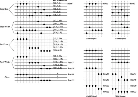
The feature selectors in Section 3have many commonalities when implemented in the unified AURA framework. We can demonstrate the commonalities by analysing 12 records from the Iris data set (Fisher, 1936). The Iris data are illustrated inFig. 6 (left) when trained into the CMM. The 12 records have been trained into a CMM using the four features and the class. Each feature is quantitative and has been subdivided into five quantisation bins of equal width.Fig. 6(right) shows the same data divided into four CMM stripes (CMMStripe1, CMMStripe2, CMMStripe3 and

CMMStripe4). The horizontal (row-based) striping means that the features ‘‘sepal len’’and ‘‘sepal width’’ are in the top stripes and ‘‘petal len’’, ‘‘petal width’’ and theclassare in the bottom two stripes. The vertical (column-based) striping means that the first 6 data records are stored in the left two stripes and the other 6 records in the right two stripes. If the data were time-series or sequential, the column-based striping would form two time frames with the oldest data in the left two stripes and the newest data in the right two stripes. The input vectors are stored in a file for each CMM or CMM stripe. These files can then be batch processed in the Hadoop framework described. Within the evaluation, we consider how the data and CMMs would be accommodated in our Hadoop framework.

MI, CFS, CS, OR and GR all useBVf_i(the binary vector where

(

F_j

=

f_i

)

),BVb_i(the binary vector representing the quantisation binbin

(

fi

)

) andBVc(the binary vector representing all records that

have class labelc). These only need to be extracted once and used in each feature selector as appropriate. For example inFig. 6, if we want all records where1

.

12

≤

petal width

<

1

.

58then we activate row 17 of the CMM. We can then Willshaw threshold the resultant integer output vectorS (000011110000) at level 1 and retrieve the binary thresholded vectorT with a bit set for every matching record (bits 4, 5, 6, 7). For the Hadoop distributed version, only the relevant CMM stripes are queried inFig. 6(right). In this case, activating row 17 ofCMMStripe3andCMMStripe4queries the relevant data.CMMStripe3will output thresholded vectorT3

with bits 5 and 6 set andCMMStripe4will outputT4with bits 7

and 8 set.T3andT4can be concatenated to form a single vector

thresholded vectorT (as inFig. 4) with bits 4, 5, 6 and 7 set. For the Hadoop distributed version, each CMM stripeCMMStripeX

outputs a list of the indices of the set bits inTXwhich are collected

by the coordinator.

CFS, GR and MI all requirenBVf_ia count of the number of data records where a particular feature has a particular valueFj

=

fi

andBVc a count of the number of records where the class has a particular labelC

=

c. To count the number of records where 1

.

12

≤

petal width

<

1

.

58, we retrieve the binary thresholded vector as above and count the number of set bits (bits 4, 5, 6 and 7 are set giving 4 matching records). For the Hadoop approach, we coordinate the retrieval as above, concatenate the lists to produce a single overall list of set bits and count the list length.T3has bits

4 and 5 set andT4has bits 6 and 7 set giving 4 matching records in

total.

CFS, CS, OR, GR and MI all use (BVf_i

∧

BVc) and (BVbi

∧

BVv)

[image:11.595.72.539.67.396.2]

V.J. Hodge et al. / Neural Networks 78 (2016) 24–35

Fig. 6. The 12 records from the iris data set, quantised and trained into a single AURA CMM (left) and subdivided across 4 stripes of the CMM (right). The letters in rows

20–22 indicate the class of the record: A=Iris-setosa, B=Iris-versicolour, C=Iris-virginica.

class isAby activating rows0and20of the CMM, thresholding

S(1222000000) at Willshaw level 2 to giveT with three bits set: column 1, 2 and 3 inFig. 6(left). This takes more coordinating in the Hadoop framework as the data for the feature value may not be stored with the data for the class; they may be in different CMM stripes. In Fig. 6 (right), activate row 0 in CMMStripe1

andCMMStripe2 and then activate row20 inCMMStripe3 and

CMMStripe4. The coordinating program needs to correlate the sections of the vector for the feature value and correlate the sections of the vector for the class to form a single vector.

CMMStripe1needs to be added (summed) with the output integer vector ofCMMStripe3to giveS1+3andCMMStripe2needs to be

added (summed) with the output integer vector ofCMMStripe4

to giveS2+4. The summed vectors can then be thresholded at 2

to giveT1+3with bits 1, 2 and 3 set (three matching records) and

T2+4with no bits set (no matches). The two thresholded output

vectors are concatenated to produceTwith bits 1, 2 and 3 set. If the thresholded vectors are stored as lists of indices (see Section4.3.1) then this is simply a task of finding the common indices between the two vectors.

MI, CFS, CS, OR and GR all also need a count of the conjunction, that isn

(

BVf_i

∧

BVc

)

and n

(

BVbi

∧

BVc

)

for qualitative and

quantitative features respectively. Hence, we retrieve the binary thresholded vectorTas above and count the set bits.

Rather than calculating these elements multiple times, we can take advantage of the commonalities by calculating each common value, binary vector or count only once and propagating the result to each feature selector that requires it. Following these common calculations, all necessary calculations will have been made for MI and GR. CFS just requires the pairwise feature versus feature

analyses (BVb_i

∧

BVb_k). These are performed in the same way as the feature versus class analyses above. CS and OR require the manipulation of some of the binary vectors to produce the logical orvectors. This requires the coordination of the vectors. To find

(

BVbi

)

∨

(

BVc

)

, we combine the list of set bits for

(

BVbi

)

with

the list of set bits for

(

BVc

)

and count the resulting list length.

By calculating the common elements first, the remainder of the calculations can be performed for each feature selector using either this CMM and processing the algorithms in series or by generating multiple copies of the CMM and processing them in parallel if sufficient processing capacity is available.

Once all of the binary vectors have been retrieved by the distributed Hadoop system, they need to be processed to calculate the feature scores as per Section 3 using the various feature selectors. A coordinator program organises this in parallel. There is one feature score calculation process per feature selector (currently five feature selectors are described here).

For the Iris data set, there are 20 feature row activations20

∗

BVbi and three class activations3

∗

BVc. To calculate (BVbi

∧

BVc) requires 20

×

3

=

60 calculations. Hence, there are 83 common calculations (20

+

3

+

60) across all five feature selectors. CFS then needs to calculate (BVbi

∧

BVbk) which would

require 19! calculations if every feature value was compared to every other. However, CFS uses greedy forward search so that the number of comparisons is minimised (Hall, 1998) to a worst case of

(

202

−

20

)/

2

=

190. We have already extracted all 20

∗

BVbi binary vectors so CFS needs 190 logicalands but no

CMM accesses. We have saved a minimum of 20 CMM accesses for

BVbiand a maximum of 190 CMM accesses for worst case forward