entropy
Article
Far-From-Equilibrium Time Evolution between Two
Gamma Distributions
Eun-jin Kim1,*ID, Lucille-Marie Tenkès1,2, Rainer Hollerbach3ID and Ovidiu Radulescu4
1 School of Mathematics and Statistics, University of Sheffield, Sheffield S3 7RH, UK;
2 ENSTA ParisTech Université Paris-Saclay, 828 boulevard des Maréchaux, 91120 Palaiseau, France
3 Department of Applied Mathematics, University of Leeds, Leeds LS2 9JT, UK; [email protected]
4 DIMNP-UMR 5235 CNRS, Université de Montpellier, Place Eugène Bataillon, 34095 Montpellier, France;
* Correspondence: [email protected]; Tel.: +44-114-222-3876
Received: 18 August 2017; Accepted: 21 September 2017; Published: 22 September 2017
Abstract:Many systems in nature and laboratories are far from equilibrium and exhibit significant fluctuations, invalidating the key assumptions of small fluctuations and short memory time in or near equilibrium. A full knowledge of Probability Distribution Functions (PDFs), especially time-dependent PDFs, becomes essential in understanding far-from-equilibrium processes. We consider a stochastic logistic model with multiplicative noise, which has gamma distributions as stationary PDFs. We numerically solve the transient relaxation problem and show that as the strength of the stochastic noise increases, the time-dependent PDFs increasingly deviate from gamma distributions. For sufficiently strong noise, a transition occurs whereby the PDF never reaches a stationary state, but instead, forms a peak that becomes ever more narrowly concentrated at the origin. The addition of an arbitrarily small amount of additive noise regularizes these solutions and re-establishes the existence of stationary solutions. In addition to diagnostic quantities such as mean value, standard deviation, skewness and kurtosis, the transitions between different solutions are analysed in terms of entropy and information length, the total number of statistically-distinguishable states that a system passes through in time.
Keywords: non-equilibrium statistical mechanics; gamma distribution; stochastic processes; Fokker-Planck equation; fluctuations and noise
1. Introduction
In classical statistical mechanics, the Gaussian (or normal) distribution and mean-field type theories based on such distributions have been widely used to describe equilibrium or near equilibrium phenomena. The ubiquity of the Gaussian distribution stems from the central limit theorem that random variables governed by different distributions tend to follow the Gaussian distribution in the limit of a large sample size [1–3]. In such a limit, fluctuations are small and have a short correlation time, and mean values and variance completely describe all different moments, greatly facilitating analysis.
Many systems in nature and laboratories are however far from equilibrium, exhibiting significant fluctuations. Examples are found not only in turbulence in astrophysical and laboratory plasmas, but also in forest fires, the stock market and biological ecosystems [4–23]. Specifically, anomalous (much larger than average values) transport associated with large fluctuations in fusion plasmas can degrade the confinement, potentially even terminating fusion operation [6]. Tornadoes are rare, large amplitude events, but can cause very substantial damage when they do occur. In biology, the pioneering work of Delbrück on bacteriophages showed that viruses replicate in strongly fluctuating bursts [24]. The fluctuations of the burst amplitudes were explained mathematically by stochastic
autocatalytic reaction models first introduced in [25]. Delbrück’s autocatalytic models predict discrete negative-binomial distributions, which can be well approximated by gamma distributions when the average number of particles is large. Furthermore, gene expression and protein productions, which used to be thought of as smooth processes, have also been observed to occur in bursts, leading to negative binomial and gamma distributed protein copy numbers (e.g., [19–23]). Such rare events of large amplitude (called intermittency) can dominate the entire transport even if they occur infrequently [8,26]. They thus invalidate the assumption of small fluctuations with short correlation time, making mean value and variances meaningless. Therefore, to understand the dynamics of a system far from equilibrium, it is crucial to have a full knowledge of Probability Distribution Functions (PDFs), including time-dependent PDFs [27].
The consequences of strong fluctuations in far-from-equilibrium systems are multiple. In physics, far-from-equilibrium fluctuations produce dissipative patterns, shift or wipe out phase transitions, etc. In economics, finance and actuarial science, strong fluctuations are important issues of risk evaluation. In biology, strong fluctuations generate phenotypic heterogeneity that helps multicellular organisms or microbial populations to adapt to changes of the environment by so-called “bet-hedging” strategies. In such a strategy, only a part of the cell population adapts upon emergence of new environmental conditions. The remaining part retains the memory of the old conditions and is thus already adapted if environmental conditions revert to previous ones [28]. Exceptional behaviour can also rescue cell subpopulations from drug-induced lethal conditions, thus generating drug resistance [29]. In particular, because of the skewness and exponential tail of the gamma distribution, gamma-distributed populations contain a significant proportion of individuals with an exceptionally high phenotypic variation. Bet-hedging being a dynamic phenomenon, it is important, for biological studies, to be able to predict not only steady-state, but also time-dependent distributions.
Obtaining good quality PDFs is often very challenging, as it requires a sufficiently large number of simulations or observations. Therefore, a PDF is usually constructed by averaging data from a long time series and is thus stationary (independent of time). Unfortunately, such stationary PDFs miss crucial information about the dynamics/evolution of non-equilibrium processes (e.g., tumour evolution). Theoretical prediction of time-dependent PDFs has proven to be no less challenging due to the limitation in our understanding of nonlinear stochastic dynamical systems, as well as the complexity in the required analysis.
Spectral analysis, for example, using theoretical tools similar to those used in quantum mechanics (e.g., raising and lower operators) is useful (e.g., [1]), but the summation of all eigenfunctions is necessary for time-dependent PDFs far from equilibrium. Various different methodologies have also been developed to obtain approximate PDFs, such as the variational principle, the rate equation method or the moment method [30–35]. In particular, the rate equation method [31,32] assumes that the form of a time-dependent PDF during the relaxation is similar to that of the stationary PDF and thus approximates a time-dependent PDF during transient relaxation by a PDF having the same functional form as a stationary PDF, but with time-varying parameters.
2. Stochastic Logistic Model
We consider the logistic growth with a multiplicative noise given by the following Langevin equation:
dx
dt = (γ+ξ)x−ex
2, (1)
wherex is a random variable andξis a stochastic forcing, which for simplicity, can be taken as a
short-correlated random forcing as follows:
hξ(t)ξ(t0)i=2Dδ(t−t0). (2)
In Equation (2), the angular brackets represent the average overξ,hξi=0, andDis the strength
of the forcing.γis the control parameter in the positive feedback, representing the growth rate ofx,
whileerepresents the efficiency in self-regulation by a negative feedback.γx−ex2can be considered
as the gradient of the potentialV asγx−ex2 = −∂∂Vx, where V = −γ2x2+ e3x3. Thus,V has its
minimum value atx = γ
e. Whenξ =0,x = γ
e (the carrying capacity) is a stable equilibrium point
since∂xxV
x=γ/e
=γ>0;x=0 is an unstable equilibrium point since∂xxV
x=0=−γ<0.
The multiplicative noise in Equation (1) shows that the linear growth rate contains the stochastic partξ. This model is entirely phenomenological, andx can be interpreted as the size of a critical
physical phenomenon (vortex, tornado, etc.), stock market, number of biological cells, viruses and proteins. It is reminiscent of Delbrück’s autocatalytic processes [25], but is different from these in many ways, the most important being the lack of discreteness and the possibility of reaching a steady-state due to the finite capacity of logistic growth. We will show in the following that in spite of these differences, our model is capable of producing large fluctuations.
By using the Stratonovich calculus [2,3,38], we can obtain the following Fokker–Planck equation for the PDFp(x,t)(see Appendix A for details):
∂
∂tp(x,t) =− ∂
∂x h
(γx−ex2)p(x,t) i
+D ∂
∂x
x ∂
∂x h
x p(x,t)i
(3)
corresponding to the Langevin Equation (1). By setting∂tp = 0, we can analytically solve for the stationary PDFs as:
p(x) = b
a
Γ(a)x
a−1e−bx, (4)
which is the well-known gamma distribution. The two parametersaandbare given bya=γ/Dand
b=e/D. The mean value and variance of the gamma distribution are found to be:
hxi= a
b =
γ
e, Var(x) =σ
2=h(x− hxi)2i= a b2 =
γD
e2 , (5)
where σ = pVar(x) is the standard deviation. We recognise hxi as the carrying capacity for a
deterministic system withξ=0. It is useful to note thathxiis given by the linear growth rate scaled
bye, while Var(x)is given by the product of the linear growth rate and the diffusion coefficient, each
scaled bye. That is, the effect of stochasticity should be measured relative to the linear growth rate.
Therefore, the case of small fluctuations is modelled by values ofDsmall compared withγand e. In such a limit,aandbare large, makingpVar(x) hxiin Equation (5). That is, the width of the
PDF is much smaller than its mean value. In this limit, Equation (4) reduces to a Gaussian distribution. To show this, we express Equation (4) in the following form:
p≡ b a
Γ(a)e
where f(x) =bx−(a−1)lnx. For largeb, we expandf(x)around the stationary pointx=xpwhere
∂xf(x) =0=b−(a−1)/xup to the second order inx−xpto find:
xp= a−1
b ∼
a
b, f(x=xp)∼a
1−lna b
, (7)
f(x)∼ f(xp) +1
2(x−xp)
2
∂xxf(x)
x=xp
=a1−lna b
+ b
2
2a
x−a b
2
. (8)
Here,a1 was used. Using Equation (8) in Equation (6) then gives us:
p∝exp
−b 2
2a
x− a b
2
∝exph−β(x− hxi)2i, (9)
which is a Gaussian PDF with mean valuehxi. Here,β=1/Var(x)is the inverse temperature, and the
variance Var(x)is given by Equation (5). Therefore, for a sufficiently smallD, the gamma distribution is approximated as a Gaussian PDF, which is consistent with the central limit theorem as smallD corresponds to small fluctuations and large system size. See also [39] for a different derivation.
AsDincreases, the Gaussian approximation becomes increasingly less valid. Indeed, even the gamma distribution becomes invalid asymptotically, whent→∞, ifD>γ; according to Equation (4),
havinga < 1 yields lim
x→0p = xlim→0
∂p
∂x = ∞. However, from the full time-dependent Fokker–Planck
Equation (3), one finds that if the initial condition satisfiesp=0 atx=0, thenp(x=0)will remain zero for all later times. As we will see, the resolution to this seeming paradox is that no stationary distribution is ever reached forD>γ, but instead, the peak approaches ever closer tox =0, without
ever reaching it.
If we are interested in obtaining stationary solutions even whenD>γ, one way to achieve that is
to return to the original Langevin Equation (1), but now include a further additive stochastic noiseη:
dx
dt = (γ+ξ)x−ex 2+
η, (10)
whereξ andηare uncorrelated and ηsatisfieshη(t)η(t0)i = 2Qδ(t−t0). The new version of the
Fokker–Planck Equation (3) then becomes:
∂
∂tp=− ∂
∂x h
(γx−ex2)p i
+D ∂
∂x
x ∂
∂x h
x pi
+Q ∂
2
∂x2p, (11)
which has stationary solutions given by:
lnp(x) =
Z (γ−D)x− ex2
Dx2+Q dx. (12)
This integral can be evaluated analytically, but the final form is not particularly illuminating. The only point to note is that for non-zeroQ, the denominator is never zero, even forx→0, which avoids any possible singularities at the origin. Forγ>DandQD, the solutions are also essentially
indistinguishable from the previous gamma distribution (4). The only significant effect of includingη
therefore is to avoid the previous difficulties at the origin whenD>γ.
satisfies this. In contrast, for (11), the appropriate boundary condition is ∂
∂xp=0 atx=0. To derive
this boundary condition for (11), we simply integrate (11) over the rangex= [0,∞]and require that the total probability should always remain one, so that dtd R p dx=0. Regarding the outer boundary, choosing some moderately large outer value for xand then imposing p = 0 there was sufficient. Resolutions up to 106grid points were used, and results were carefully checked to ensure they were independent of the grid size, time step and precise choice of outer boundary.
3. Diagnostics
Once the time-dependent solutions are computed, we can analyse them using a number of diagnostics. First, we can evaluate the mean valuehxiand standard deviationσfrom (5). Next, to explore the extent to
which the time-dependent PDFs differ from gamma distributions, we can simply compare them with ‘equivalent’ gamma distributions and compute the difference. That is, givenhxiandσ, the gamma
distributionpequivhaving the same mean and variance would have as its two parametersa=hxi2/σ2
andb=hxi/σ2. With these values, we define:
Difference= Z
|p−pequiv|dx (13)
to measure how different the actual time-dependent PDF is from its equivalent gamma distribution. Two other familiar quantities often useful in analysing PDFs are the skewness and kurtosis, defined by:
Skewness= h(x− hxi) 3i
σ3 , Kurtosis=
h(x− hxi)4i
σ4 −3. (14)
Skewness measures the extent to which a PDF is asymmetric about its peak, whereas kurtosis measures how concentrated a PDF is in the peak versus the tails, relative to a Gaussian having the same variance (the−3 is included in the definition of the kurtosis to ensure that a Gaussian would yield zero). For gamma distributions, one finds analytically that the skewness is 2pD/γ, and the kurtosis is 6D/γ.
Comparing the skewness and kurtosis of the time-dependent PDFs with these formulas is therefore another useful way of quantifying how similar or different they are from gamma distributions.
Another quantity that can be useful is the so-called differential entropy as a measure of order versus disorder (as entropy always is):
S=− Z
plnp dx. (15)
In particular, we expectSto be small for localised PDFs and large for spread out ones (e.g., [40–43]). For unimodal PDFs as the ones studied here, entropy and standard deviation are typically comparably good measures of localization, but for bimodal peaks, entropy can be significantly better [42]. For the gamma distribution in Equation (4), the differential entropy can be shown to be given by:
S=a−lnb+ln(Γ(a)) + (1−a)ψ(a), (16)
whereψ(a) = dln(dxΓ(x))
x=ais the double gamma function.
Our final diagnostic quantity is what is known as information length. Unlike all the previous diagnostics, which are simply evaluated at any instant in time, but otherwise do not involve t, information length is a Lagrangian quantity, explicitly concerned with the full time-history of the evolution of a given PDF. It is thus ideally suited to understanding time-dependent PDFs. Very briefly, we begin by defining:
E ≡ 1
[τ(t)]2 =
Z 1
p(x,t)
∂p(x,t) ∂t
2
dx. (17)
Note howτhas units of time and quantifies the correlation time over which the PDF changes, thereby
information in time.E is due to the change in either width (variance) of the PDF or the mean value, which are determined byγ,Dandefor the gamma distribution (e.g., see Equation (4)). In the standard
Brownian motion, the mean value is zero so thatE is due to the change in the variance of a PDF. The total change in information between initial and final times, zero andtrespectively, is then defined by measuring the total elapsed time in units ofτas:
L(t) = Z t
0 dt1 τ(t1)
= Z t
0 s
Z
dx 1
p(x,t1)
∂p(x,t1) ∂t1
2
dt1. (18)
This information lengthLmeasures the total number of statistically distinguishable states that a system evolves through, thereby establishing a distance between the initial and final PDFs in the statistical space. Note thatLby construction is a continuous variable and thus measures the total “number” of statistically-different states as a continuous number. See also [40–48] for further applications and theoretical background ofEandL.
4. Results
4.1.γ>D
We start with the caseγ>D, where Equation (3) has stationary solutions, given by (4). Keepinge
andDfixed, we then switchγback and forth between two values, in the following sense: Take the
gamma distribution (4) corresponding to one value; call itγ1; and use that as the initial condition to
solve (3) with the other value; call itγ2. We then interchangeγ1andγ2to complete the pair of “inward”
and “outward” processes. Such a pair can be thought of as an order/disorder phase transition [40,41], caused for example by cyclically adjusting temperature in an experiment. This protocol is also inspired from adaptation of a biological system. During adaptation, a model parameter can be abruptly changed in response to the change of environmental conditions, for instance a particle replication parameterγ,
but the resulting changes can be extremely heterogeneous in the population.
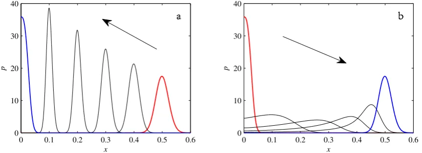
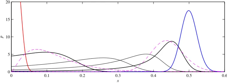
Figure1shows the result of switchingγbetweenγ1 =0.5 andγ2 =0.05, for fixede=1 and
D=0.02 (one of the three parameterse,γandDcan of course always be kept fixed by rescaling the
entire equation, so throughout this entire section, we keepe=1 fixed and focus on how the various
quantities depend onγandD). We immediately see that the inward and outward processes behave
differently. Whenγis decreased and the peak therefore moves inward, the PDF is relatively narrow,
and the peak amplitude is monotonically increasing. Whenγis switched from 0.05 back to 0.5, the PDF
is much broader, and the peak amplitude in the intermediate stages is less than either the initial or final gamma distributions.
0 0.2 0.4 0.6 0.8 0
4 8 12 16
x
p
0 0.2 0.4 0.6 0.8
0 4 8 12 16
x
p
[image:7.595.87.512.86.244.2]a
b
Figure 1.(a) shows the result of switchingγ=0.5→0.05; (b)γ=0.05→0.5, both at fixede=1 and
D=0.02. The initial (red) and final (blue) gamma distributions are shown as heavy lines. The four intermediate lines are when the time-dependent solutions havehxi=0.1, 0.2, 0.3, 0.4. The arrows are a reminder of the direction of motion, inward on the left and outward on the right.
10−2 100 102 0
0.1 0.2 0.3 0.4 0.5
t
<x>
10−2 100 102 10−5
10−4 10−3 10−2 10−1
t
E
⋅
D
10−2 100 102 10−2
10−1 100
t
L
⋅
D
1/2
a
b
c
Figure 2. (a) showshxias a function of time; (b) showsE ·D (to indicate theE ∼ D−1 scaling); (c) showsL ·D1/2(to indicate theL ∼D−1/2scaling). Solid lines denoteγ=0.5→0.05, dashed lines
the reverse. Each solid or dashed “line” is in fact three, occasionally barely distinguishable, lines with
D=0.01, 0.02, 0.04. The dots on thehxicurves correspond to the PDFs shown in Figure1.
ForE andL, the equilibration is again somewhat slower forγ =0.5 →0.05 than the reverse.
We can further identify clear scalingsE ∼D−1andL ∼D−1/2. Finally,Lis greater forγ=0.5→0.05
than the reverse. These results are all understandable in terms of the interpretation ofLas the number of statistically-distinguishable states that the PDF evolves through: First, we recall from Figure1
thatγ=0.5→0.05 had consistently narrower PDFs than the reverse. Narrower PDFs means more
distinguishable states, hence largerLforγ=0.5→0.05 than the reverse. TheL ∼D−1/2scaling has
the same explanation; smallerDyields narrower PDFs, hence largerL.
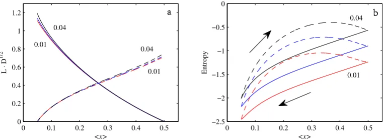
The first panel in Figure3shows the previous quantitieshxiandL ·D1/2, but now plotted against each other rather than separately against time. The behaviour is exactly as one might expect, with Lgrowing more or less linearly with distance from the initial position. The right panel in Figure3
shows the entropy (15), again as a function ofhxirather than time, to emphasize the cyclic nature of the two processes. The significance is indeed as claimed above, with more localized PDFs having smaller entropy values. Note howγ=0.5→0.05, which had the narrower PDFs, has lower entropy
[image:7.595.93.510.315.474.2]0 0.1 0.2 0.3 0.4 0.5 0
0.2 0.4 0.6 0.8 1 1.2
0.01 0.01
0.04 0.04
<x>
L
⋅
D
1/2
0 0.1 0.2 0.3 0.4 0.5
−2.5 −2 −1.5 −1 −0.5 0
0.01 0.04
<x>
Entropy
[image:8.595.108.490.87.227.2]a b
Figure 3.(a) showsL ·D1/2and (b) entropy, both as functions ofhxi. Solid lines denoteγ=0.5→0.05,
dashed lines the reverse. Numbers besides curves indicateD=0.01, 0.02, 0.04. The arrows on the entropy plot are a reminder of the direction of inward/outward motion.
Figure4shows how the standard deviation, skewness and kurtosis behave, again, as functions ofhxithroughout the two processes. The heavy green lines also show the behaviour that would be expected if the time-dependent PDFs were always gamma distributions throughout their evolution. That is, if gamma distributions have hxi = γ, σ =
√
γD, skewness = 2pD/γ and kurtosis =
6D/γ (setting e = 1), then expressed as functions of hxi, we would have (σ/D1/2) = phxi,
(skewness /√D) =2/phxiand (kurtosis /D) =6/hxi. As we can see, theγ=0.5→0.05 process
follows these functional relationships reasonably well (especially for skewness and kurtosis), but for
γ=0.05→0.5, all three quantities deviate substantially.
0 0.1 0.2 0.3 0.4 0.5 0.2
0.4 0.6 0.8
<x>
σ
/ D
1/2
0.01
0.04
0 0.1 0.2 0.3 0.4 0.5 0
2 4 6 8 10
<x>
Skewness / D
1/2
0.01 0.04
0 0.1 0.2 0.3 0.4 0.5 0
20 40 60 80 100 120
<x>
Kurtosis / D
0.01 0.04
[image:8.595.91.514.411.566.2]a
b
c
Figure 4. (a)σ/D1/2, (b) (skewness /D1/2) and (c) (kurtosis /D), as functions ofhxi. Solid lines
denoteγ=0.5→0.05, dashed lines the reverse. Numbers besides curves indicateD=0.01, 0.02, 0.04.
The heavy green curves arephxi, 2/phxiand 6/hxi, respectively, and indicate the behaviour expected for exact gamma distributions.
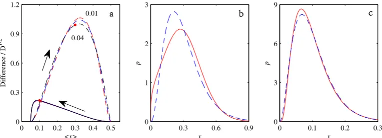
Further evidence of significant deviations from gamma distribution behaviour is seen in Figure5, showing the difference (13) directly. As expected from Figure4,γ=0.05→0.5 has a much greater
difference thanγ=0.5→0.05. The second and third panels show how the PDFs compare with the
equivalent gamma distributions having the samehxiandσvalues as the actual PDFs at that instant.
0 0.1 0.2 0.3 0.4 0.5 0
0.3 0.6 0.9 1.2
0.04 0.01
<x>
Difference / D
1/2
0 0.3 0.6 0.9
0 1 2 3
x
p
0 0.1 0.2 0.3
0 3 6 9
x
p
[image:9.595.107.490.86.225.2]a b c
Figure 5.(a) shows the difference (13) between the actual PDF and the equivalent gamma distribution, as functions ofhxi. Solid lines denoteγ= 0.5→ 0.05, dashed lines the reverse, with arrows also
indicating the direction of motion. The dots athxi = 0.3 forγ = 0.05 → 0.5 andhxi = 0.1 for
γ=0.5→0.05, correspond to the other two panels: (b) compares theγ=0.05→0.5 PDF with its
equivalent gamma distribution; (c) compares theγ =0.5 → 0.05 PDF with its equivalent gamma
distribution. The actual PDFs in each case are solid (red), and the equivalent gamma distributions are dashed (blue).D=0.04 for both sets.
4.2. D>γ
We next consider the case D > γ, where we demonstrated above that stationary solutions
cannot exist at all, because the time-dependent PDF can only ever get closer and closer to the gamma distribution singularity at the origin, but can never actually achieve it. To explore what does happen in this case then, we simply repeat the above procedure, except that there is now only an ‘inward’ process, and no reverse. That is, instead ofγ = 0.5 →0.05, let us considerγ = 0.5 →0 (Throughout this
section, we will also takeD=10−3, to facilitate comparison with results in the next section. Forγ=0,
of course, anyDis greater thanγ.).
Figure 6 shows the resulting PDFs and how they approach ever closer to the origin, but never actually achieve thex−1 blow-up that would be implied by Equation (4) for a = γ/D = 0.
The peak amplitude simply increases indefinitely, ast1/2. The widths correspondingly also decrease; the apparent increase is an illusion caused by the logarithmic scale forx. The dashed lines also show the equivalent gamma distributions, as before. Note how the difference becomes increasingly noticeable; in line with the fact that the equivalent gamma distribution is tending toward its singular behaviour as hxidecreases, but the actual PDFs must always havep(0) =0.
10−5 10−4 10−3 10−2 10−1 100
101
102
103
0 1 3 10 30 100
300 1000
x
[image:9.595.108.490.562.702.2]p
Figure 6.The initial condition is a gamma distribution withγ=0.5,e=1 andD=10−3;γis then
Figure7is the equivalent of Figure2and directly comparesγ=0.5→0 here with the previous γ=0.5→0.05. We see thathxistarts out very similarly, but instead of equilibrating to 0.05, it now
tends to zero ast−1.E again starts out similarly, but ultimately tends to zero much more slowly, ast−3 instead of exponentially. Thist−3scaling forEhas an interesting consequence forL, namely thatL does saturate to a finite valueL∞(sinceR
t−3/2dtremains bounded fort→∞) even though the PDF itself never settles to a stationary state.
10−1 101 103
10−3 10−2 10−1 100
t
<x>
10−1 101 103
10−9 10−6 10−3 100
t
E
⋅
D
10−1 101 103
10−2 10−1 100
t
L
⋅
D
1/2
a
b
c
Figure 7.As in Figure2, (a) showshxi; (b) showsE ·D; and (c)L ·D1/2. Solid lines denoteγ=0.5→0
forD=10−3, dashed lines the previousγ=0.5→0.05 forD=0.01. Note how the scalings ofEand LwithDare still preserved even whenDis changed by a factor of 10.
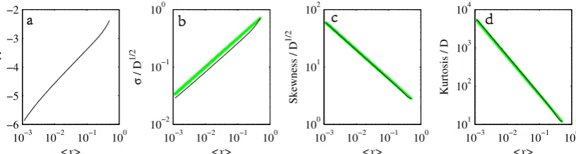
Figure8shows entropy,σ, skewness and kurtosis, so some of the results as in Figures3and4.
Entropy andσare again both good measures of how narrow the PDF is, becoming ever smaller as the
peak moves toward the origin. Skewness and kurtosis seem to follow the expected gamma distribution relationship extremely well, even though we saw before in Figure6that the PDFs are actually different from gamma distributions. Ashxi →0, both skewness and kurtosis thus become indefinitely large.
10−3 10−2 10−1 100 −6
−5 −4 −3 −2
<x>
Entropy
10−3 10−2 10−1 100 10−2
10−1 100
<x>
σ
/ D
1/2
10−3 10−2 10−1 100 100
101 102
<x>
Skewness / D
1/2
10−3 10−2 10−1 100 101
102 103 104
<x>
Kurtosis / D
[image:10.595.96.504.484.593.2]a
b
c
d
Figure 8.(a) Entropy, (b)σ/D1/2, (c) (skewness /D1/2) and (d) (kurtosis /D), as functions ofhxi, for
theγ=0.5→0 calculation from Figure6. The heavy green curves in the last three panels arephxi,
2/p
hxiand 6/hxi, respectively, and indicate the behaviour expected for exact gamma distributions.
4.3. Q6=0
Finally, we turn to the Fokker–Planck Equation (11) with additive noise included and use it to explore the two questions that could not be addressed otherwise. First, how does a process like
γ = 0.5 → 0 then equilibrate to a stationary solution? Second, what does the reverse process
γ=0→0.5 look like?
dominant only withinx≤0.1; any stationary solutions with peaks much beyond that are effectively pure gamma distributions.
Figure9 shows the same type of inward/outward process as before in Figure1, only now switchingγbetween 0.5 and 0.1. Comparing with Figure1, we see that the dynamics are very similar,
just with all the peaks considerably narrower, which is to be expected ifD=10−3rather than 0.02. The only other point to note is how the final peak in the left panel is lower than the previous peak at hxi=0.2, which is different from Figure1, whereγ=0.5→0.05 had peaks monotonically increasing
throughout the entire evolution. The reason for the final peak here decreasing slightly is precisely the influence ofQin this region; if this peak is now seeing just as much diffusion fromQas fromD, it is not surprising that it spreads out somewhat more and is correspondingly somewhat lower than a pure gamma distribution would be.
0 0.1 0.2 0.3 0.4 0.5 0.6
0 5 10 15 20 25 30
x
p
0 0.1 0.2 0.3 0.4 0.5 0.6
0 5 10 15 20 25 30
x
p
[image:11.595.109.489.248.388.2]a b
Figure 9. (a) shows the result of switchingγ= 0.5→ 0.1, (b)γ = 0.1→ 0.5, both at fixede = 1,
D=10−3andQ=10−5. The initial (red) and final (blue) gamma distributions are shown as heavy lines. The three intermediate lines are when the time-dependent solutions havehxi=0.2, 0.3, 0.4. L∞=25 on the left and 16 on the right.
Figure10shows the fundamentally new case, namely switchingγbetween 0.5 and zero. The inward
processγ=0.5→0 is again very similar to either Figure1or9. The only difference from Figure6
is that the process does actually equilibrate to a stationary solution now, as given by Equation (12). The reverse processγ=0→0.5 is rather different though. The initial central peak now broadens far
more than previously seen in Figures1and9.
0 0.1 0.2 0.3 0.4 0.5 0.6 0
10 20 30 40
x
p
0 0.1 0.2 0.3 0.4 0.5 0.6 0
10 20 30 40
x
p
[image:11.595.83.515.543.700.2]a
b
Figure 10.(a) the result of switchingγ=0.5→0, (b)γ=0→0.5, both at fixede=1,D=10−3and
One interesting consequence of this extreme broadening forγ=0→0.5 is on the total information
lengthL∞. In Figure9, these values are 25 and 16, respectively, whereas in Figure10, they are 35 and 9.5. That is, in both cases, decreasingγyields largerL∞values than increasingγdoes, consistent
with the peaks being narrower, hence passing through more statistically-distinguishable states. Next, comparingL∞ = 25 forγ = 0.5 → 0.1 versus 35 for γ = 0.5 → 0, this is exactly as one might
expect: having the peak travel somewhat further yields extra information length. However, comparing L∞=16 forγ=0.1→0.5 versus 9.5 forγ=0→0.5 is puzzling then. The peak has further to travel,
but accomplishes it with less information length. The reason is precisely this extreme broadening, which substantially reduces the number of distinguishable states along the way. See also [40,41], where the same effect was studied for Gaussian PDFs and values ofDas small as 10−7, leading to
fundamentally different scalings ofL∞withDfor inward and outward processes.
Returning to the central question of this paper, namely how close the time-dependent PDFs are to gamma distributions, the results for Figure9are similar to the previous ones. In particular, we recall that before in Figure5, we had the difference scaling asD1/2, so a smallerDhere means a smaller
difference. These results are approaching the smallDregime where gamma distributions become very close to Gaussians anyway, which generally remain close to Gaussian as they move.
However, for theγ=0→0.5 process in Figure10, the intermediate stages do not look much like
gamma distributions (the final equilibrium is indistinguishable from a gamma distribution though, consistent withQbeing completely negligible for these values ofx). For the intermediate stages, these were found to be so different from gamma distributions that attempting to fit a gamma distribution having the samehxiandσmade little sense; this extreme broadening and long tail trailing behind the
peak meant that bothhxiandσwere too different from the normal expectation that they should be
measures of ‘peak’ and ‘width’.
Instead, we simply asked the question, which values ofaandbwould minimize the quantity
R
|p−pbf|dx, wherepis the time-dependent PDF to be fitted andpbfis the best-fit gamma distribution.
Unlike our previous difference formula, this does not yield simple analytic formulas for theaandbto choose, but is numerically still straightforward to implement. Figure11shows the results, for two of the intermediate stages in theγ=0→0.5 process. We can see that the fit is rather poor, indicating
that these PDFs are significantly different from gamma distributions.
This misfit is also not caused by the inclusion ofQ; if this or any similar central peak is evolved for either small or zeroQin the Fokker–Planck equation, the result is always similar to here. As explained also in [40,41], the dynamics of how central peaks move away from the origin is simply different from how peaks already away from the origin move, regardless of whether the final states are Gaussians as in [40,41] or gamma distributions as here.
0 0.1 0.2 0.3 0.4 0.5 0.6
0 5 10 15 20
x
[image:12.595.107.487.559.699.2]p
Figure 11. Theγ =0 → 0.5 process as in Figure10, but now shown in more detail. The dashed
5. Conclusions
Gamma distributions are among the most popular choices for modelling a broad range of experimentally-determined PDFs. It is often assumed that time-dependent PDFs can then simply be modelled as gamma distributions with time-varying parametersaandb. In this work, we have demonstrated that one should be cautious with such an approach. By numerically solving the full time-dependent Fokker–Planck equation, we found that there are three sets of circumstances where the PDFs can differ significantly from gamma distributions:
• IfD < γ, so that stationary solutions exist, butDis also sufficiently close toγthat a gamma
distribution differs significantly from a Gaussian, then the time-dependent PDFs will also differ significantly from gamma distributions.
• IfD>γ, stationary gamma distributions do not exist at all. Instead, peaks move ever closer to
the origin and in the process increasingly differ from gamma distributions.
• If the initial condition is a peak right on the origin—either as a result of adding additive noise to produce stationary solutions even forD> γ, or simply as an arbitrary initial condition—then
any evolution away from the origin will differ significantly from gamma distributions. Unlike the previous two items, which become more pronounced for largerD, this effect is most clearly visible for smallerD, where the mismatch between the naturally narrower peaks and the extreme broadening seen in Figure11becomes increasingly significant.
In summary, our results show that a simple Langevin equation model mimics the strong fluctuations of far-from-equilibrium systems. This model has gamma distributions as steady-state solutions, but the time-dependent solutions can deviate considerably from this law. This makes tasks such as Bayesian and frequentist inference of the model from data more complicated. On the other hand, the model shows complex asymptotic dynamics with situations when a steady state is reached or not, different from the one of the deterministic logistic model that invariably evolves to the maximum capacity. The studied model is general enough and can be applied to many practical situations in biology, economics, finance and physics. Future work will apply some of these ideas to fitting actual data.
Author Contributions:Eun-jin Kim and Rainer Hollerbach conceived the basic mathematical ideas; Ovidiu Radulescu provided background in biology and other areas; Eun-jin Kim conducted the analytical derivations; Lucille-Marie Tenkès and Rainer Hollerbach conducted the numerical calculations; all authors were involved in writing the paper. All the authors have read and approved the final manuscript.
Conflicts of Interest:The authors declare no conflict of interest.
Appendix A. Derivation of the Fokker–Planck Equations
In order to derive the Fokker–Planck Equation (3) from the Langevin Equation (1), it is useful to introduce a generating functionZ:
Z=eiλx(t). (A1)
Then, by definition of ‘average’, the average ofZis related to the PDF,p(x,t), as:
hZi= Z
dx Z p(x,t) = Z
dx eiλx(t)p(x,t). (A2)
Thus, we see thathZiis the Fourier transform ofp(x,t). The inverse Fourier transform ofhZithen givesp(x,t):
p(x,t) = 1
2π Z
dλe−iλxhZi. (A3)
We note that Equation (A3) can be written as:
p(x,t) =
1 2π
Z
dλeiλ(x−x(t))
which is another form ofp(x,t). To obtain the equation forp(x,t), we first derive the equation forhxi and then take the inverse Fourier transform as summarised in the following.
We differentiateZwith respect to timetand use Equation (1) to obtain:
∂tZ=iλ∂txZ=iλ(γx−ex2+ξ(t)x)Z=λ[γ∂λ+ie∂λλ+ξ∂λ]Z, (A5)
wherexZ=−i∂λZwas used. The formal solution to Equation (A5) is:
Z(t) =λ Z
dt1[γ∂λ+ie∂λλ+ξ(t1)∂λ]Z(t1). (A6)
The average of Equation (A5) gives:
∂thZi=λ(γ∂λ+ie∂λλ)hZi+λhξ(t)∂λZ(t)i. (A7)
To findhξ(t)∂λZ(t)i, we use Equation (A6) iteratively as follows:
hξ(t)∂λZi =
ξ(t)∂λ
λ Z
dt1 [γ∂λ+ie∂λλ+ξ(t1)∂λ]Z(t1)
= hξ(t)i∂λ
λ Z
dt1 [γ∂λ+ie∂λλ]hZ(t1)i
+∂λ
λ Z
dt1hξ(t)ξ(t1)i∂λhZ(t1)i
= ∂λ
h
λ[D∂λhZ(t)i] i
. (A8)
Here, we used the independence ofξ(t)andZ(t1)fort1<t,hξ(t)Z(t1)i=hξ(t)ihZ(t1)i=0, together
with Equation (2),R0tdt1δ(t−t1) =1/2, andhξi=0. By substituting Equation (A8) into Equation (A7),
we obtain:
∂thZi=λ(γ∂λ+ie∂λλ)hZi+λ∂λ
h
λ[D∂λhZ(t)i]
i
. (A9)
The inverse Fourier transform of Equation (A9) then gives us:
∂
∂tp(x,t) =− ∂
∂x h
(γx−ex2)p(x,t) i
+D ∂
∂x
x ∂
∂x h
x p(x,t)i
(A10)
which is Equation (3). Specifically, the inverse Fourier transforms of the first and last terms in Equation (A9) are shown explicitly in the following:
1 2π
Z
dλe−iλxh∂tZi=∂t
1 2π
Z
dλe−iλxhZi
= ∂
∂tp(x,t), (A11)
D 2π
Z
dλe−iλxλ∂λ[λ∂λhZi] =D ∂ ∂x
x ∂
∂x h
x p(x,t)i
, (A12)
where integration by parts was used twice in obtaining Equation (A12). The additionalQ∂xxpterm in the Fokker–Planck Equation (11) can be derived in the same way.
Appendix B. Time-Dependent Analytical Solutions of Equation (3)
We begin by making the change of variablesy=1/xin Equation (1) to obtain:
dy
dt =−(γ+ξ)y+e. (A13)
By using the Stratonovich calculus [2,3,38], the solution to Equation (A13) is found as:
y(t) =y0e−(γt+B(t))+ee−(γt+B(t)) Z t
0 dt1e
wherey0=y(t=0)andB(t) = Rt
0 dt1ξ(t1)is the Brownian motion. Therefore,
x(t) = x0e
γt+B(t)
1+ex0
Rt
0dt1e(γt1+B(t1))
, (A15)
where x0 = x(t = 0). In Equation (A15), eB(t) is the geometric Brownian motion whilee−γt−B(t)
is the geometric Brownian motion with a drift (e.g., [2]). The time integral of the latter is used in understanding stochastic processes in financial mathematics and many other areas [49,50]. In particular, in the long time limit, its PDF can be shown to be a gamma distribution. However, this PDF ofxis not particularly useful as it involves complicated summations and integrals that cannot be evaluated in closed form [49,50].
References
1. Risken, H.The Fokker-Planck Equation: Methods of Solution and Applications; Springer: Berlin, Germany, 1996. 2. Klebaner, F.Introduction to Stochastic Calculus with Applications; Imperial College Press: London, Britain, 2012. 3. Gardiner, C.Stochastic Methods, 4th ed.; Springer: Berlin, Germany, 2008.
4. Saw, E.-W.; Kuzzay, D.; Faranda, D.; Guittonneau, A.; Daviaud, F.; Wiertel-Gasquet, C.; Padilla, V.; Dubrulle, B. Experimental characterization of extreme events of inertial dissipation in a turbulent swirling flow.
Nat. Commun.2016,7, 12466, doi:10.1038/ncomms12466.
5. Kim, E.; Diamond, P.H. On intermittency in drift wave turbulence: Structure of the probability distribution function.Phys. Rev. Lett.2002,88, 225002.
6. Kim, E.; Diamond, P.H. Zonal flows and transient dynamics of the L-H transition.Phys. Rev. Lett.2003,90, 185006. 7. Kim, E. Consistent theory of turbulent transport in two dimensional magnetohydrodynamics.Phys. Rev. Lett.
2006,96, 084504.
8. Kim, E.; Anderson, J. Structure-based statistical theory of intermittency.Phys. Plasmas2008,15, 114506. 9. Newton, A.P.L.; Kim, E.; Liu, H.-L. On the self-organizing process of large scale shear flows.Phys. Plasmas
2013,20, 092306.
10. Srinivasan, K.; Young, W.R. Zonostrophic instability.J. Atmos. Sci.2012,69, 1633–1656.
11. Sayanagi, K.M.; Showman, A.P.; Dowling, T.E. The emergence of multiple robust zonal jets from freely evolving, three-dimensional stratified geostrophic turbulence with applications to Jupiter.J. Atmos. Sci.2008,
65, 3947–3962.
12. Tsuchiya, M.; Giuliani, A.; Hashimoto, M.; Erenpreisa J.; Yoshikawa, K. Emergent self-organized criticality in gene expression dynamics: Temporal development of global phase transition revealed in a cancer cell line.
PLoS ONE2015,10, e0128565.
13. Tang, C.; Bak, P. Mean field theory of self-organized critical phenomena.J. Stat. Phys.1988,51, 797–802. 14. Jensen, H.J.Self-Organized Criticality: Emergent Complex Behavior in Physical and Biological Systems; Cambridge
University Press: Cambridge, UK, 1998.
15. Pruessner, G.Self-Organised Criticality; Cambridge University Press: Cambridge, UK, 2012.
16. Longo, G.; Montévil, M. From physics to biology by extending criticality and symmetry breaking.
Prog. Biophys. Mol. Biol.2011,106, 340–347.
17. Flynn, S.W.; Zhao, H.C.; Green, J.R. Measuring disorder in irreversible decay processes.J. Chem. Phys.2014,
141, 104107.
18. Nichols, J.W.; Flynn, S.W.; Green, J.R. Order and disorder in irreversible decay processes.J. Chem. Phys.2015,
142, 064113.
19. Ferguson, M.L.; Le Coq, D.; Jules, M.; Aymerich, S.; Radulescu, O.; Declerck, N.; Royer, C.A. Reconciling molecular regulatory mechanisms with noise patterns of bacterial metabolic promoters in induced and repressed states.Proc. Natl. Acad. Sci. USA2012,109, 155–160.
20. Shahrezaei, V.; Swain, P.S. Analytical distributions for stochastic gene expression.Proc. Natl. Acad. Sci. USA
2008,105, 17256.
21. Thomas, R.; Torre, L.; Chang, X.; Mehrotra, S. Validation and characterization of DNA microarray gene expression data distribution and associated moments.BMC Bioinform.2010,11, 576.
22. Iyer-Biswas, S.; Hayot, F.; Jayaprakash, C. Stochasticity of gene products from transcriptional pulsing.
23. Elgart, V.; Jia, T.; Fenley, A.T.; Kulkarni, R. Connecting protein and mRNA burst distributions for stochastic models of gene expression.Phys. Biol.2011,8, 046001.
24. Delbrück, M. The burst size distribution in the growth of bacterial viruses (bacteriophages). J. Bacteriol.
1945,50, 131.
25. Delbrück, M. Statistical fluctuations in autocatalytic reactions.J. Chem. Phys.1940,8, 120–124.
26. Kim, E.; Liu, H.; Anderson, J. Probability distribution function for self-organization of shear flows.
Phys. Plasmas2009,16, 052304.
27. Kim, E.; Hollerbach, R. Time-dependent probability density function in cubic stochastic processes.Phys. Rev. E
2016,94, 052118.
28. De Jong, I.G.; Haccou, P.; Kuipers, O.P. Bet hedging or not? A guide to proper classification of microbial survival strategies.Bioessays2011,33, 215–223.
29. Balaban, N.; Merrin, J.; Chait, R.; Kowalik, L.; Leibler, S. Bacterial persistence as a phenotypic switch.Science
2004,305, 1622–1625.
30. Glansdorff, P.; Prigogine, I. Thermodynamic theory of structure, stability and fluctuations.Am. J. Phys.1973,
41, 147–148.
31. Suzuki, M. Microscopic theory of formation of macroscopic order.Phys. Lett. A1980,75, 331–332.
32. Suzuki, M. The variational theory and rate equation method with applications to relaxation near the instability point.Phys. A Stat. Mech. Appl.1981,105, 631–641.
33. Langer, J.S.; Baron, M.; Miller, H.D. New computational method in the theory of spinodal decomposition.
Phys. Rev. A1975,11, 1417.
34. Saito, Y. Relaxation in a bistable system.J. Phys. Soc. Jpn.1976,61, 388–393.
35. Hasegawa, H. Variational approach in studies with Fokker-Planck equations.Prog. Theor. Phys.1977,58, 128–146. 36. Dennis, B.; Costantino, R.F. Analysis of steady-state populations with the gamma abundance model:
Application to Tribolium.Ecology1988,69, 1200–1213.
37. Liao, H.-Y.; Ai, B.-Q.; Hu, L. Effects of multiplicative colored noise on bacteria growth.Braz. J. Phys.2007,37, 1125–1128.
38. Wong, E.; Zakai, M. On the convergence of ordinary integrals to stochastic integrals.Ann. Math. Stat.1960,
36, 1560–1564.
39. Bagui, S.C.; Mehra, K.L. Convergence of binomial, Poisson, negative-binomial, and gamma to normal distribution: Moment generating functions technique.Am. J. Math. Stat.2016,6, 115–121.
40. Kim, E.; Hollerbach, R. Geometric structure and information change in phase transitions.Phys. Rev. E2017,
95, 062107.
41. Hollerbach, R.; Kim, E. Information geometry of non-equilibrium processes in a bistable system with a cubic damping.Entropy2017,19, 268.
42. Tenkès, L.-M.; Hollerbach, R.; Kim, E. Time-dependent probability density functions and information geometry in stochastic logistic and Gompertz models.arXiv2017, arXiv:1708.02789.
43. Frieden, B.R.Physics from Fisher Information; Cambridge University Press: Cambridge, Britain, 2000. 44. Wootters, W.K. Statistical distance and Hilbert space.Phys. Rev. D1981,23, 357.
45. Nicholson, S.B.; Kim, E. Investigation of the statistical distance to reach stationary distributions.Phys. Lett. A
2015,379, 83–88.
46. Nicholson, S.B.; Kim, E. Structures in sound: Analysis of classical music using the information length.
Entropy2016,18, 258, doi: 10.3390/e18070258.
47. Heseltine, J.; Kim, E. Novel mapping in a non-equilibrium stochastic process.J. Phys. A2016,49, 175002. 48. Kim, E.; Lee, U.; Heseltine, J.; Hollerbach, R. Geometric structure and geodesic motion in a solvable model of
non-equilibrium stochastic process.Phys. Rev. E2016,93, 062127.
49. Bertoin, J.; Yor, M. Exponential functionals of Lévy processes.Prob. Surv.2005,2, 191–212.
50. Matsumoto, H.; Yor, M. Exponential functionals of Brownian motion, I: Probability laws at fixed time.
Prob. Surv.2005,2, 312–347.
c