This is a repository copy of Long Memory Affine Term Structure Models. White Rose Research Online URL for this paper:
http://eprints.whiterose.ac.uk/99262/ Version: Accepted Version
Article:
Golinski, Adam orcid.org/0000-0001-8603-1171 and Zaffaroni, Paolo (2016) Long Memory Affine Term Structure Models. Journal of Econometrics. pp. 33-56. ISSN 0304-4076
https://doi.org/10.1016/j.jeconom.2015.09.006
[email protected] https://eprints.whiterose.ac.uk/
Reuse
This article is distributed under the terms of the Creative Commons Attribution-NonCommercial-NoDerivs (CC BY-NC-ND) licence. This licence only allows you to download this work and share it with others as long as you credit the authors, but you can’t change the article in any way or use it commercially. More
information and the full terms of the licence here: https://creativecommons.org/licenses/
Takedown
If you consider content in White Rose Research Online to be in breach of UK law, please notify us by
Long Memory Affine
Term Structure Models
⇤
Adam Goli´
nski
Paolo Zaffaroni
This draft: 6th September 2015
Abstract
We develop a Gaussian discrete time essentially affine term structure model with long memory state variables. This feature reconciles the strong persistence observed in nominal yields and inflation with the theoretical implications of affine models, especially for long maturities. We characterise in closed-form the dynamic and cross-sectional implications of long memory for our model. We explain how long memory can naturally arise within the term structure of interest rates, providing a theoretical underpinning for our model. Despite the infinite-dimensional structure that long memory implies, we show how to cast the model in state space and estimate it by maximum likelihood. An empirical application of our model is presented.
JEL classification: G12, C58 ,C32.
Key words: Gaussian essentially affine model, long memory, state space, P and Q mea-sures.
∗We are grateful to the Editor (Yacine Ait-Sahalia), the Associate Editor and two anonymous referees for
1.
Introduction
One of the main challenges in modelling the term structure of interest rates is the fact that nominal observed yields are extremely persistent. In fact, they are essentially non-distinguishable from a non-stationary series: any test would hardly reject the hypothesis of a unit root. Although explicitly assumed in early work of term structure modelling (see Dothan (1978)), accepting the possibility of a unit root in the physical measure appears troublesome in terms of its economic implications and econometric estimation. In fact, the unit root paradigm rules out any degree of mean-reversion, namely the possibility that shocks are eventually absorbed as time goes by. Lack of mean-reversion bears implausible cross-sectional predictions, in particular in terms of the volatility term structure of yields, forwards and holding period returns. In terms of estimation, the possibility of a unit root affects the finite sample as well as the asymptotic properties of conventional estimators of term structure models, making inference more difficult.
Recognising that the notion of long memory permits to obtain a substantial degree of persistence, in fact even non stationarity, together with dynamic mean-reversion, this paper develops a class of discrete time no-arbitrage affine term structure models with long memory state variables. The idea of long memory has been postulated as a suitable description of nominal yields by Backus and Zin (1993), which can be seen as a very special case of our general theory.
Our long memory model belongs to the class of essentially affine (in the sense of Duffee (2002)) Gaussian term structure models with multiple, possibly latent, factors. We establish the closed-form solution of the general model and, relying on its state space representation, show how to carry out estimation by maximum likelihood and Kalman filtering when latent state variables are allowed for. These achievements are non trivial because an important feature of long memory models is to be non-Markov implying infinite-dimensional state variables.
Our approach shares the many virtues of the powerful class of affine models, pioneered by Vasicek (1977) and Cox et al (1985) highly influential models and formally defined by Duffie and Kan (1996). First, closed-form solution for bond prices and yields can be obtained as affine functions of a set of state variables. Second, nominal yields can be decomposed into inflation expectations, real yields and inflation risk premia with minimal, no-arbitrage, as-sumptions. Third, conditional moments, in particular term premia, can be easily computed. Fourth, the model can be naturally cast in state-space implying that parameters estima-tion and inference can be obtained by maximum likelihood estimaestima-tion. Filtered values of the latent state variables, which typically include expected inflation and the short-term real interest rate, follow by the Kalman recursion.
To better understand the analogies and differences of our model with the conventional affine models, it is useful to consider the unified framework represented by the classDAQM(N) of discrete time affine models spelled out by Le et al (2010), where M of the N factors (here 0 M N) drive the stochastic volatility.1 Gaussian affine models, whereby the
unconditional distribution of the state vectors is normal, feature M = 0 (no stochastic 1This class nests all the exact discrete time representation of the general class of continuous time models
volatility) and makes theDAQ0(N) class. A crucial feature of theDAQ0(N) class is that, under the risk-neutral (hereafterQ) measure, theN state variables form a Markov system, possibly of higher yet finite order such as a vector autoregression (hereafter VAR). It is well known that the Markov property together with stationarity, under the physical measure, implies a weak form of temporal dependence for model-implied yields, as expressed by the fast decay toward zero of their autocorrelation function.2 At the same time, a stationary VAR under
the Q measure implies that the theoretical volatility, both conditional and unconditional, of long yields and forwards diminishes fast toward zero as maturity increases. Instead, the theoretical volatility of holding period returns stays bounded for large maturities. These features are completely at odds with the empirical evidence. However, if one relaxes the assumption of stationarity under the Q measure, within this DAQ0(N) class, a unit or even an explosive root emerges, of which the consequences are also at odds with the empirical evidence: the theoretical (conditional) volatility of yields and forwards either flattens out (in the unit root case) or increase sharply (in the explosive root case) across maturity. For returns a sharp increase is always obtained.
In contrast, due to the long memory specification of our model, we are able to match the strong degree of persistence together with the dynamic mean-reversion observed in nom-inal yields. At the same time, the model-driven term structures of volatility, for yields and forwards, can be slowly decaying for intermediate maturities yet flattening out or even (slowly) increasing for long maturities. Instead, the model-driven volatility term structure will diverge for returns. Unlike the Markov case, these implications are now compatible with mean-reversion. More importantly, these are the features observed in the data. As we shall see, long memory can be obtained by allowing the dimension of state vector, N, to become infinite, spanning the DAQ0(1) class of term structure models, with respect to the Le et al (2010) notation. Besides infinite-dimensionality of the state variables, a suitable long lags characterization of the state variables impulse response is required in order to induce long memory.
Long memory has been explored by Comte and Renault (1996), who develop a continuous time long memory model of the term structure, and by Duan and Jacobs (1996) where long memory enters through the volatility of the state variables. More recently, Abbritti et al (2015) and Osterrieder (2013) proposed Gaussian term structure models with observed-only state variables whose dynamics follow a suitably restricted vector autoregression with long memory. Latent factors are not permitted in either models which can be seen as different, particular cases, of our general approach.3 In particular, Abbritti et al (2015)
emulate long memory by a long finite-order vector autoregression of order k (with k up to 100) with a long memory parameterization of the coefficients. Theoretical properties of the model are standard since, by all means, it is an affine model with a finite set of observed
2Theorem 1 of Chan and Palma (1998) shows this result in the general set up of a linear state space with
a finite dimensional state vector.
3 Given observability of the state variables, both Abbritti et al (2015) and Osterrieder (2013) estimate
state variables satisfying a k-th order VAR. The market price of risk dynamics is specified as an affine function of the state variables vector and, due to the long lags specification, depends onO(k2) parameters, most of which are zeroed for practical estimation. Osterrieder
(2013) considers fractional cointegrating restrictions of the dynamics of the state variables, which must exhibit the same degree of long memory, using recent advances in the theory of fractional cointegration. This model provides a genuine long memory specification but the analysis is simplified by the assumption of constant market prices of risk, implying the equivalence of the Q and P measures in terms of second moments.
Since Rogers (1997), it is well known that assuming long memory for a tradable asset might lead to existence of arbitrage opportunities. This would undermine the possibility to identify the pricing kernel and thus, in our case, to determine model-implied (bond) prices. However, it is now understood that the conditions required to violate no-arbitrage are much more stringent in a discrete time setting such as ours (see Cheridito (2003)). Moreover, arbitrage opportunities are ruled out whenever transaction costs, no matter how minimal, are allowed for, ensuring existence and uniqueness of the pricing kernel (see Guasoni et al (2010)). Therefore, as discussed below, in practice no pricing consequence for our model appears to arise despite its long memory feature.
The paper proceeds as follows. Section 2 describes the data for nominal yields and macro variables used for estimation of the model. We highlight some features of the yields data, namely their dynamic persistence and the shape of their volatility term structure, es-pecially for long maturities. Section 3 explores the extent to which these features can be accounted for by Vasicek-type model, spelling out the theoretical implication for long term yields, forwards and returns. This paves the ground for the model presented in Section 4: a multi-factor discrete time essentially affine non-Markov Gaussian term structure model with long memory. Section 4.2 provides in closed-form the analytical characterization of the time series and cross-sectional properties, in terms of volatility term structure, for model-implied yields, forwards and holding period returns, under various forms of the market price of risk. A review of different approaches to tackle the high persistence of observed nominal yields and their analogies with our long memory approach are discussed in Section 5. Section 6 discusses theoretical underpinnings of long memory in real and nominal yields, leaving some formal details to Appendix A. Section 7 presents estimation results for a version of our model that includes realised inflation and real activity as observed state variables. This makes such specifications of our model akin to term structure models that merge yields and macroeco-nomic data, such as theDAQ0(N)-type models of Ang and Piazzesi (2003), Rudebush and Wu
(2008) and Hordhalh et al (2008) among others.4 It is also asked for by the data. In fact long
memory appears to be a robust description of realised inflation dynamics. Altissimo et al (2009) analyse how the consumer price index (hereafter CPI) construction protocol gives rise naturally to long memory in CPI inflation and provide empirical evidence for the inflation
4Although not pursued in the current paper, including inflation is instrumental for recovering the canonical
rate of the euro area. As a consequence, inflation appears to be one of the main channels that naturally leads to long memory in observed nominal yields, as argued below. We verify in Section 7 that the above described features of the empirical distribution of zero coupon bonds are extremely well matched by the estimated model. Final remarks make Section 8. Appendix A explains the mechanics of how long memory can be induced within the class of affine term structure models. Appendix B discusses the pricing implications of long memory for our model. A technical description of the Kalman filter and an approximate maximum likelihood estimator for long memory processes is relegated to Appendix C. Appendix D contains some technical lemmas and the proofs of the main theorems.
2.
Some stylised facts of nominal bonds
We now highlight the well established strong degree of dynamic persistence that charac-terises certain specific aspects of the empirical distribution of nominal bonds. We consider the term structure of nominal yields, forwards and holding period returns. This strong persistence appears to be the main channel through which the negligible volatility of bond returns at very short maturities becomes magnified by several orders of magnitude as we move along the term structure. Similarly, the riskiness of long term yields and forwards appear only slowly declining along the term structure, far from vanishing for very long ma-turities. At first glance, these stylised facts can be qualitatively rationalised by means of a simple Markov term structure model, as exemplified in Section 3. However, when looking more carefully, both the time series and the cross-sectional evidence appears at odds with the quantitative predictions of such term structure model built around both stationary and non-stationary Markov state variables.
We use a data set comprised of monthly observations of nominal yields y$
n,t on zero
coupon bonds with maturities n equal to 1 month and 1,3,5,10,15,20 and 30 years. The 1-month yield comes from the Fama’s Treasury Bills Term Structure files while, for all other maturities, yields are extracted from the data of Gurkaynak et al (2007). We consider the period from January 1986 to December 2011.5 Yields
y$
ni,t=− 1
ni
logP$ nit
are continuously compounded, annualised and expressed in percent, whereP$
nitdenotes nom-inal zero coupon bond prices with maturity ni. We also consider (nominal) forward rates
fn$i,ni+1,t = (ni+1yn$i+1,t−niy
$
ni,t)/(ni+1−ni) with maturities ni < ni+1, and holding period returns
rn$i
−1,ni,t= (niy
$
ni,t−(ni−ni−1)−ni−1y
$
ni−1,t)/(ni−ni−1) with maturities ni−1 < ni, 5Gurkaynak et al (2007) report the 30-year yield curve estimates since 25 November 1985, which is
referring to them as f$
ni,t and r
$
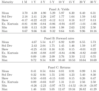
ni,t in the standard, monthly, case when ni+1−ni = 1. The latter (monthly figure) is the case considered in our empirical analysis. Summary statistics are presented in Table 1.
[Insert Table 1 near here]
Average yields are increasing with maturity whereas their volatility, expressed in terms of standard deviation, shows a hump at about one year maturity, decreases and then slightly increases again. A similar pattern is obtained in terms of forwards, the main difference being that for forwards their volatility term structure raises even more for long maturities after declining from the one-year hump. Holding period returns exhibit a monotonically increasing volatility curve.
It has been known for a long time that nominal yields display a substantial degree of persistence.6 This is evident when performing unit root tests, illustrated in Table 2, where
we present the results for the standard Augmented Dickey-Fuller (ADF) unit root test. The null hypothesis of a unit root is not rejected for nominal yields across all maturities.
[Insert Table 2 near here]
We propose to assess the persistence of nominal bonds using a somewhat more sophisti-cated approach that does not suffer the limits of the unit root framework. In particular, we need to use a measure that allows to disentangle the notion of non-stationarity from the one of mean-reversion.
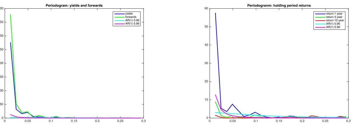
Figure D and Figure D plot the periodogram ordinates near the zero frequency, respec-tively, for yields (blue line) and forwards (green line) averaged across maturity,7 and for
returns at 1- (blue line), 10- (green line) and 30-year maturity (red line), where for a sample of generic observables (w1, ...wT) the periodogram is
Iw(λ) =
1 2πT
! ! ! ! !
T
X
t=1
wteıλt
! ! ! ! !
2
, −π < λ π,
where ıdefines the complex unit. Data have been standardised so that the sample variance is unity.
[Insert Figure 1 near here]
The strength of using the periodogram comes essentially from the fact that it is a nonpara-metric measure, that uses the information of the entire string of sample autocorrelations of the data.8 More generally, it gives neat insights on both the low, medium and high frequency
dynamics of the data, which in turn are linked to the long run persistence, mean-reversion and cycles of the data. For instance, the periodogram near zero frequency is proportional to the sum of the entire set of sample autocorrelations corresponding to a given sample and,
6See for example Ball and Torous (1996) and Kim and Orphanides (2012) among many others. 7The same pattern is observed for the single maturities with little variation.
as such, is a clearcut measure of long run persistence.9 Instead, the local behaviour of the
periodogram, as one moves away from the zero frequency, provides indication on the degree of mean-reversion. Finally, cycles induce local peaks at the corresponding frequencies within the interval [−π, π].
To provide a benchmark, any stationary autoregressive moving average (ARMA) process implies a bounded spectral density, flattening out near the zero frequency. We plot the spectral density for AR(1) model with unit variance with autoregressive parameter equal to 0.90 (purple line) and 0.99 (light blue line), in both Figures D and D together with the periodogram of yields, forwards and returns.
The results are strikingly clear. Yields and forwards are very persistent, much more than an AR(1) model with coefficient equal to 0.99. A similar feature, although with a smaller dis-crepancy, applies to holding period returns with 1-year maturity. In contrast, as the maturity lengthens, returns appear much less persistent. Indeed the persistence diminishes (mono-tonically) as the maturity increases: the 10-year return appears approximately described by an AR model with a positive autoregressive coefficient whereas the 30-year return appears no persistent at all. This comparison is compelling: even a value of the AR coefficient as large as 0.99 does not induce a sufficiently large degree of persistence able to match the peak found in the periodogram of the data near the zero frequency. The mean-reversion implied by stationary ARMA is also too strong. On the other hand, an AR(1) model with a coefficient so close to unity, would be hard to be distinguished from a unit root using any conventional unit root test. The problem with the unit root paradigm is that it does induce persistence but at the cost of giving up stationarity and, in particular, mean-reversion. This provides implausible predictions for the volatility cross-section of nominal bond characteristics across maturities, as discussed below.
We summarize this finding as follows.
Stylized Fact 1. Nominal yields and forwards, at all maturities, and nominal holding period
returns, for small maturities, are highly persistent and mean reverting across time: their periodogram displays a peak near the zero frequency and quickly diminishes when away from the zero frequency. The persistence of nominal holding period returns diminishes substantially with maturity.
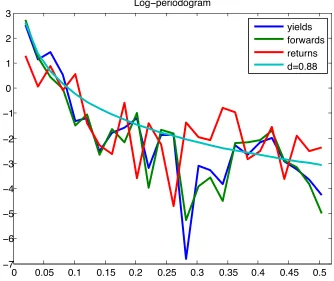
As an alternative, more precise, characterization of persistence found in the data, one can state that nominal yields, forwards and holding period returns (for short maturities) have an approximately linear negatively sloped log periodogram near the origin, slowly decaying as the frequency increases. Anticipating matters explained subsequently, if the data are characterized by a unit root, such negative slope would be approximately minus two. If instead the data were generated by a stationary ARMA this slope would be zero. In practice, careful examination of the data reveals a slope smaller than zero. We will explain these concepts below once we articulate the notion of long memory.
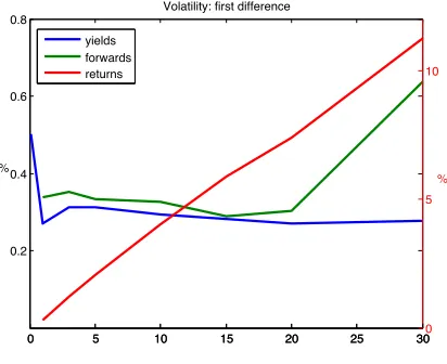
Figure D displays the term structure of the sample standard deviations of yields (blue line), forwards (green line) and returns (red line). As observed in Table 1, for yields the curve
9The periodogram can be rewritten asI
w(λ) = (1/2⇡)P T−1
k=−T+1covˆ w(k)eıkλ forλ6= 0 where ˆcovw(k) = T−1PT−|k|
t=1 (wt−w¯)(wt+|k|−w¯), namely the sample autocovariance at lagk(see Brockwell and Davis (1991),
initially increases up to 1-year maturity, then it decays and, finally, it slightly increases for longer maturities. Forward rates have a similar pattern, although they show a more substantial increase toward the end of the term structure. Clearly for both yields and forwards the volatility is not vanishing at long maturity. Instead, the term structure of the sample standard deviation of holding period returns raises steeply with maturity. If non-stationarity is suspected, one can instead consider the term structure of the sample standard deviations of the first difference of yields, forwards and returns. The results are presented in Figure D, where for the first difference of yields and forwards their sample standard deviation is multiplied by 10, to better see the pattern. It turns out that the term structures of volatility of first-differenced yields, forwards and returns show essentially the same pattern (although with a different scale) as for the raw quantities, with now (first-differenced) forwards exhibiting a more clear raise at long maturities, as opposed to yields.
[Insert Figure 2 near here]
These observations lead to:
Stylized Fact 2. The term structure of the sample standard deviation of nominal yields
and forwards increases at short maturities with hump at around 1-year. They then decrease but eventually slowly increase for very long maturities. The term structure of the sample standard deviation of nominal holding period returns rises sharply with maturity without flattening out.
These facts are well documented in the term structure literature. Note that although
Stylized Fact 1is a time series characteristic,Stylized Fact 2 features cross-sectional aspects of the bond data. However, these are intimately related and can be rationalised within an affine framework. The approach proposed in this paper tries to explain both features.
3.
Implications for Markov affine models
We now revisit the theoretical implications of the persistence of yields found in the data for Gaussian Markov affine models. For the sake of expository purpose, consider the discrete time version of the Vasicek (1977) model, a one-factor Gaussian model, here applied to nominal yields. The price of a nominal zero coupon bond issued at time t which expires n
periods ahead satisfies the no-arbitrage condition
Pn,t$ =Et
⇣
em$t+1P$
n−1,t+1
⌘
, (1)
where Et(·) is the expectation operator conditional on the information available up to time
t, based on the physical measure. It is well-known that no-arbitrage implies existence of the (nominal) pricing kernel em$t+1, the exponent of which, for this model, has the simple form
−m$t+1 =δ0+
1 2λ
2
where the (single) factor follows an AR(1) process
xt=ψxxt−1+εx,t, where the εx,t are N ID(0, σ2x), (3)
and the market price of risk is affine in the factor:
λt =λ0+λ1xt, (4)
with λ0, λ1, δ0, ψx, σx2 constant parameters. Stationarity of xt requires |ψx|<1.
By the standard recursive method one obtains that bond yields y$
n,t, forward rates fn,t$
and holding one-period returns r$
n,t satisfy, respectively,
yn,t$ = n−1(An$ +Bn$xt), (5)
fn,t$ = A$n+1−A$n+ (Bn+1$ −Bn$)xt, (6)
rn,t$ = A$n−A$n−1 +Bn$xt−1−Bn−1$ xt, (7)
where, in turn, the affine function coefficients satisfy the well-established Riccati difference equations:
A$n=A$n−1+δ0−λ0σ2xBn−1$ −
1 2(B
$
n−1)2σ2x and Bn$ = 1 +ψQxBn−1$ , (8)
with initial conditionsA$
0 =B0$ = 0, where we define theQ-measure autoregressive coefficient
ψQ
x =ψx−λ1σx2.
Consider first the stationary case |ψx| < 1.10 Clearly yields, forwards and returns are
affine transformations of the AR(1) process xt, and their temporal dependence, under the
physical measure, is determined by the magnitude ofψx. Analytically, the spectral densities
for yields, forwards and returns are,11 for −π λ < π,
syn(λ) = (
B$ n
n )
2s x(λ),
sfn(λ) = (B
$
n−Bn−1$ )2sx(λ),
srn(λ) = (1−λ1σ
2
x)2sx(λ) + (B$n−1)2
σ2 x
2π −2(1−λ1σ
2
x)Bn−1$ ψ−1x
σ2 x
2π< ✓
1 1−ψxeıλ
−1
◆ ,
where<(.) denotes the real part of a complex number andsx(λ) indicates the spectral density
of the AR(1) state variable (3), equal to σ2
x/(2π|1−ψxeıλ|2). By easy derivations, the slope
10Stationarity of yields, forwards and returns is driven by the physical measure autoregressive coefficients x. The Q-measure autoregressive coefficient xQ only enters into the construction of the loadings A
$ n, B
$ n
and, in particular, determines the behaviour of the variances for largen.
11For returnsr$
n,tthe additional terms in the spectral density are due to the fact thatr $
n,tcan be represented
asA$
n−A
$
n−1+ (1−λ1σ2x)xt−1−Bn$−1"x,t. However the behaviour of the first and third term insrn(λ) are
of the log spectra, for λ !0+, will then satisfy
dlog syn(λ)
dlogλ ⇠ −
2ψx
(1−ψx)2
λ2, dlog sfn(λ)
dlogλ ⇠ −
2ψx
(1−ψx)2
λ2, dlog srn(λ)
dlogλ ⇠ −2 ✓
(1−λ1σ2x)2
(1−ψx)2
−B$ n−1
◆−2
(1−λ1σx2)2ψx
(1−ψx)2
− B
$
n−1(1−λ1σ2x)
(1−ψx)2
! λ2,
where ⇠ indicates asymptotic equivalence.12 In all cases the slope becomes null at zero frequency and its magnitude, near zero frequency, is larger the closer ψx is to unity.
The term structures of conditional and unconditional volatility for yields, forwards and returns are
vart−1(yn,t$ ) =
⇣B$ n
n ⌘2
σx2, var(yt,n) =
⇣B$ n
n
⌘2 σ2 x
1−ψ2 x
,
vart−1(fn,t$ ) = (ψ
Q
x)2nσ2x, var(ft,n) = (ψxQ)2n
σ2 x
1−ψ2 x
,
vart−1(rn,t$ ) = (Bn$)2σx2, var(rt,n) = (Bn$)2σ2x+
σ2 x
1−ψ2 x
,
where vart(·) is the physical measure variance operator conditional on the information
avail-able up to time t. Notice that the behaviour of the variances across maturity n is driven by the Q-measure autoregressive coefficient ψQ
x. Since Bn$ ⇠ 1/(1−ψQx) for large n when
|ψQ
x|<1, it follows that, as n! 1,
vart−1(y$n,t)⇠
✓ σ2
x
(1−ψxQ)2
◆
1
n2, vart−1(f $
n,t)⇠(ψxQ)2nσx2, vart−1(rn,t$ )⇠
σ2 x
(1−ψxQ)2
. (9)
An identical pattern is obtained for the unconditional variances. Finally, consider now the case |ψQ
x| ≥1. Obviously this does not imply that the model is truly non-stationary under
the physical measure since stationarity depends on ψx. The term structure of conditional
volatility for yields, forwards and returns will now be vart−1(y$t,n) = σx2, vart−1(ft,n$ ) =
σ2
x, vart−1(r$t,n) = n2σx2whenψQx = 1 whereas vart−1(yt,n$ )⇠
⇣
σ2 x
(ψQx)2−1
⌘
n−1(ψQ
x)2n, vart−1(ft,n$ )⇠
(ψQ
x)2nσ2x, vart−1(rt,n$ )⇠
⇣
σ2 x
(ψQx)2−1
⌘
(ψQ
x)2n when ψxQ >1. Therefore, the volatility curves of
yields and forwards will either decay very quickly (towards zero) or diverge very quickly for large maturities, depending on whether ψQ
x is smaller or bigger than unity. The model is
whereas non-stationarity, either a unit or explosive root, rules out mean-reversion altogether. Moreover, postulating a unit root invalidates the evaluation of impulse responses and vari-ance decomposition. There appears the need for a model able to generate an intermediate degree mean-reversion between these two cases, without imposing stationarity. This is ac-complished by the long memory affine term structure model, which we formalise in the next section.
4.
Long memory affine term structure models:
repre-sentation
Long memory models, in particular autoregressive fractionally integrated moving average (ARFIMA) models, bridge the gap between stationary ARMA and ARIMA (when a unit root is allowed for). In fact, not only can long memory models describe the dynamics of stationary yet highly persistent time series but can also account for non-stationary yet mean reverting series, whereby the impulse response function will eventually die out with time.13 There is another, less known, feature of linear long memory models that makes them
particularly useful with respect to affine models, namely the fact that they admit a state-space representation although with infinite-dimensional state variables. This result has been established by Chan and Palma (1998) and summarized in Appendix C. More importantly, it turns out that, despite the presence of an infinite number of transition equations, the likelihood can be computed in a finite number of steps. Therefore parameter estimates can be obtained and the Kalman filter delivers optimal forecasts. Moreover, the model can accomodate latent factors, which in turn can be optimally recovered by the Kalman filter. The possibility of allowing latency of the factors is particularly important for the purpose of term structure modelling, since it opens up the possibility of estimating the real term structure, the expected inflation term structure and the associated risk premia.
These considerations suggest to consider Gaussian affine models with long memory state variables. This model is described in the following subsections. We first show how to solve the model imposing the no-arbitrage condition for a general specification of the model, yet providing a closed-form solution. We then consider specific parameterizations, such as ARFIMA, which are required in order to carry our estimation.
4.1. General multi-factor model
In this section we will refer to nominal yields for illustrative purposes but the model will apply to either nominal and real yields. The interpretation of the results would clearly differ. However, adopting some slight modifications, the model can also be used to decompose nominal yields in real yields, inflation expectations and inflation risk premia based on the same data set.
Assume that the (nominal) short rate is driven by K factors xt = (x1,t, ..., xK,t)0:
yt,1$ =δ0+δ0xt, (10)
with coefficients δ = (δ1, δ2, ..., δK)0 and intercept δ0. Some, none or all the factors could be
latent, although this is not relevant in terms of representation. We then assume that the (nominal) stochastic discount factor m$
t is a quadratic function of theK factors:
−m$t+1 =yt,1$ + 1 2λ
0
tΣλt+λ0tεt+1 (11)
through the market prices of risk λt, which are affine in the state variables
λt=
0 B @
λ1,t
...
λK,t
1 C
A=λ0+λ1xt (12)
for aK⇥1 vectorλ0 and aK⇥K matrixλ1 = (λ1.1...λ1.K) withjth columnλ1.j. Formulation
(12) qualifies the model as ‘essentially’ affine. The vector of innovations εt is assumed i.i.d.
with
εt=
0 B @
ε1,t
...
εK,t
1 C
A⇠N ID(0,Σ). (13)
Expression (11) for the pricing kernel is implied by the existence of a conditionally log-normal stochastic process αt = αt−1exp(−0.5λ0t−1Σλt−1 −λ0t−1εt) such that EtQ(Xt+1) =
α−1t Et(Xt+1αt+1) for any stochastic process Xt+1, where EtQ(·) defines the conditional
ex-pectation operator under the Q measure (see Harrison and Kreps (1979)). Hereafter, we shall specify all model equations and parameters in terms of the physical measure, un-less stated otherwise. Since the price of any (nominal) asset that does not pay dividends is a martingale under Q (once adjusted by e−y$t), for nominal zero coupon bond prices
P$ n,t =E
Q
t [e−y
$ tP$
n−1,t+1] =Et[e−y
$ tP$
n−1,t+1αt+1/αt] =Et[Pn−1,t+1$ em
$ t+1].
To close the model one needs to specify the dynamics of the factors (under the physical measure). In order to introduce long memory, we need to make a distinction between factors and state variables. The dynamics of each factor xj,t, with 1j K, is more conveniently
represented by the infinite-dimensional state vectorsCj,t which obey an infinite-dimensional
VAR(1) model
Cj,t+1 =FCj,t+hjεj,t+1, 1j K, (14)
for an infinite-dimensional vector hj and a double-infinite dimensional matrix F. Notice
that the innovations in (14) are the same as in (13) and are, therefore, contemporaneously correlated throughΣ. This implies that each state vectorCj,t is influenced by the overall set
of lagged state vectorsC1,s, . . . ,CK,s for everyst. Equations (14) represent the transition
equations of the state-space of the model used for the Kalman filter recursion. Obviously we could have written theK equations jointly asCt+1 =F⇤Ct+h⇤εt+1 for certain matrices
F⇤ and h⇤ suitably restricted, but it is more convenient to rely on (14). The relationship
between factors and state variables is simply
for an infinite dimensional vector G = (1,0, 0· · ·)0 with all zeros from the second row
onwards. Recall that the elements ofεtare in general cross-correlated (unlessΣis diagonal)
and thus the Cj,t are not independent across j.
Despite the infinite dimension of the state variables, the model can be solved along the same way used for the basic model of Section 3. We report the following result without proof.
Theorem 4.1. For the pricing kernel (11), the market price of risk (12) and the state
variable dynamics (14), the no-arbitrage zero coupon bond prices P$
n,t satisfy, by Gaussianity
(13),
p$
n,t =−A$n−B$01,nC1,t−....−B$0K,nCK,t,
where p$
n,t = lnPn,t$ and the coefficients satisfy the Riccati recursions
A$n = A$n−1+δ0 −
1 2B
$0
n−1ΣB$n−1−B$0n−1Σλ0, (16)
B$j,n = ⇣δj−B$0n−1Σλ1.j
⌘
G+F0B$j,n−1, 1j K. (17)
setting the K dimensional vector
B$n= (B$01,nh1, ...,B$0K,nhK)0.
Note thatA$
n is scalar,B$n isK dimensional and theB$j,n are infinite-dimensional vectors
for every 1 j K. These coefficients must be interpreted as being evaluated under the Q-measure unless in (12) one sets λ0 = 0 for A$
n or λ1 = 0 for the B$j,n. For these
special cases, the corresponding coefficients are interpreted to be evaluated under the P measure. The distribution of ‘observed’ bond prices and yields, viz. the physical measure, is of course function of both the P- and Q-measure parameters. As explained below, the dynamic properties of the latent factors xj,t depend on the chosen parameterization for hj
which, in turn, determines the degree of persistence and mean-reversion of the model. Nominal yields would then be obtained as
y$n,t=−n−1pn,t$ =n−1A$n+n−1B$01,nC1,t+...+n−1B$0K,nCK,t, (18)
The short term interest rate (10) will then be equal to the one-period (nominal) yield y1,t$ , obtained when A$0 = 0 and B$j,n =0 for all 1 j K. Nominal forward rates and holding period returns are given by
fn,t$ =A$n+1−A$n+ (B$1,n+1−B$1,n)0C1,t+...+ (B$K,n+1−B$K,n)0CK,t, (19)
r$n,t =A$n−A$n−1+ (B$01,nC1,t−1 −B1,n−1$0 C1,t) +...+ (B$0K,nCK,t−1−B$0K,n−1CK,t). (20)
4.2. Persistence characterization
fact that conditional moments, rather than unconditional moments, are required to solve the model for any given maturity. We now discuss possible choices for the vectors hj which
define both the degree of memory, and possibly of stationarity, of the model factors xj,t
through (14). These choices define the time series and cross-sectional properties of yields, forwards and holding period returns implied by the term structure model.
Throughout the paper we will maintain the assumption that the matrix F satisfies (see Appendix C)
F=
2 6 4
0 1 0 · · ·
0 0 1 0 ... ... . .. ...
3 7
5, (21)
By Gaussianity the factors can be expressed as linear processes in the i.i.d. innovations εj,t
of (13):
xj,t = 1
X
i=0
φj,iεj,t−i, 1j K. (22)
Recall that the εj,t−i are contemporaneously cross-correlated though the covariance matrix
Σ. Stacking together the coefficients φj,i gives the infinite dimensional vector
hj = (1 φj,1 φj,2 φj,3...)0, 1j K. (23)
Stationarity of factor xj,t follows if
1
X
i=0
φ2j,i <1. (24)
As explained below, the stationarity condition (24) includes a wide range of possibilities in terms of the degree of persistence, in turn expressed by the rate at which the coefficientsφj,i
go to zero. We briefly summarise such possibilities including the case when the stationarity condition (24) is violated. Given (22), factorxj,t will be defined short memory if
1
X
i=0
|φj,i|<1. (25)
Alternatively, factor xj,t is said to be long memory if s
X
i=0
|φj,i|! 1 as s! 1. (26)
the mean reverting case, namely when (24) is violated and yet
φj,i !0 as i! 1, (27)
and the case when even mean-reversion (27) does not occur. A simple example of this last, extreme, circumstance is given by the basic model of Section 3 when factor xt = x1,t is a
random walk, namely φ1,i = 1 for alli.
4.2.1. Short memory
We now check that the simple model of Section 3 is nested within the general solution of Section 4.1 . Set K = 1 and xt=x1,t, εt=ε1,t with δ1 = 1. Now the infinite dimensional
vector (23) equals
h1 = (1 ψx ψ2x ψ3x...)0, (28)
where ψx is the autoregressive parameter in (3). By standard arguments model (3) can be
re-written as
x1,t= 1
X
i=0
ψxiε1,t−i, (29)
implying that, obviously, the AR(1) satisfies the linearity assumption (22) with coefficients
φ1,i=ψix. When |ψx |<1 then the short memory condition (25) is satisfied, and thus both
the stationarity and the mean-reversion conditions apply. Instead, when ψx = 1 the AR(1)
becomes a random walk and even (27) fails.
One just needs to find the scalar sequence An and the infinite dimensional sequences
B$
1,n, solution of the recurrence equations (16)-(17), and verify that indeed the basic affine
model (5) is re-obtained. By (21), recursion (17) becomes
B$1,n = (1−B$n−1κ1)G+F0B$1,n−1
settingκ1 = Σλ1,Bn$ =B$01,nh1, with initial conditionB$1,0 =0yieldingB1,n = (bnbn−1. . . b10. . .)0
where
B$1,1 = (1,0, . . .)0,B$1,2 = (1−κ1,1,0, . . .)0,B$1,3 = (1−κ1(ψx+1−κ1),1−κ1,0, . . .)0, . . . (30)
A few algebraic steps giveB$0
1,nh1 = 1+ψQx+...+(ψQx)n−1 = (1−(ψxQ)n)/(1−ψxQ) for every n ≥
1 which in turn givesA$
n =A$n−1+δ0−λ0σ2xBn−1$ −12σ 2
x(Bn−1$ )2, which coincides exactly with
(8). Notice that C1,t can be expressed as
C1,t = (Et(x1,t), Et(x1,t+1), Et(x1,t+2), ...)0
where Et(x1,t+i) = P1j=iψjxε1,t+i−j for all i= 0,1, ... (see Appendix C). In turn, this implies
B$01,nC1,t= n−1
X
i=0
bn−iEt(x1,t+i) = n−1
X
i=0
bn−i 1
X
j=i
ψjxε1,t+i−j
!
=
n−1
X
i=0
bn−iψxi 1
X
j=i
ψxj−iε1,t+i−j
!
which coincides with B$
nx1,t re-obtaining the solution of Section 3. This shows that the
general solution (18) and the particular one (5) coincide when (28) holds.
4.2.2. Long memory
A particularly convenient long memory parameterization, that nests both stationary ARMA as well as the random walk is the ARFIMA model. In particular, the generic factor
xj,t follows a stationary ARFIMA(1, d,1) model (see Brockwell and Davis (1991), Definition
12.4.2) when
(1−ψjL)(1−L)djxj,t = (1 +θjL)εj,t, (31)
where the autoregressive and moving average coefficientsψj, θj satisfy the usual stationarity
and invertibility conditions
|ψj |<1, |θj |<1, with ψj 6=θj, (32)
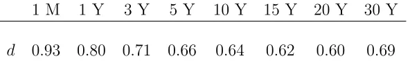
and dj is a real number such that
−1/2< dj <1/2. (33)
When (32) and (33) hold, it can be shown (see Brockwell and Davis (1991), Theorem 12.4.2) that xj,t admits the linear representation (22) with coefficients φj,i=φj,i( ξj) satisfying
1
X
i=0
φj,iLi = (1 +θjL)(1−ψjL)−1(1−L)−dj (34)
function of the vector ξj = (ψj, θj, dj)0. To discuss the stationarity and memory properties
of the factorxj,t, we use the property
φj,i ⇠c idj−1 as i! 1, (35)
which stems from (34) for any dj <1, for a constant c. Stationarity (24) then follows when
(33) holds. Short memory (25) requires dj 0 and long memory dj >0.14 As a particular
case of short memory, stationary ARMA(1,1) is obtained for dj = 0. Although stationarity
implies mean-reversion, the opposite is not necessarily true since mean-reversion (27) simply requiresdj <1. Finally, whendj = 1 one obtains the non stationary ARIMA(1,1,1) process,
a special case of which is the random walk (when ψj =θj = 0). Specification (31) extends
to ARFIMA(p, d, q) whenever ψj(L)(1−L)djxj,t =θj(L)εj,t for polynomials ψj(L), θj(L) of
orderp, q, respectively, with roots bigger than one in absolute value. This will be the general specification adopted for the factors xj,t in the empirical illustration below.
Alternative definitions of long memory when 0 < dj <1/2, equivalent to (35) for linear
stationary processes, are in terms of autocovariance function and spectral density,
respec-14Cased
j <0 is technically defined as anti-persistence, but it can be thought of as a special case of short
tively expressed as
cov(xj,t, xj,t+u)⇠c u2dj−1, as u! 1, and sj(λ)⇠c λ−2dj, as λ!0. (36)
4.3.
P
and
Q
measure implications of long memory
We now provide a quasi-closed form characterization of the general solution for bond prices as from Theorem 1. This permits to explore the implications of the long memory model in terms of dynamic persistence of yields, forwards and returns and in terms of the cross-sectional behaviour of their volatility.
Our interest is in the characterization of the physical measure, namely the ‘true’ distri-bution, of observed bond prices and transformation of such as yields, forwards and holding period returns, as can be obtained by an ideal historical observation of these quantities in the market. Assuming that the model is correctly specified, the physical distribution of bond prices will be, generally speaking, a function of both the Pand theQmeasure’s parameters. By this we mean that observed (log) bond prices are function of the loadings coefficients, namely the A$
n and the B$j,n, which are evaluated under the Q measure, and of the state
variables Cj,t, which are evaluated under the P measure.15
The results below indicate a clear dichotomy, namely that the P measure’s parameters determine the ‘long-run’ time series properties of bond prices whereas the Q measure’s pa-rameters contribute to the ‘long maturity’ cross-sectional properties of bond prices. In other words, the dynamic persistence induced by the model on the physical measure does not depend on the form of the market prices of risk or, generally speaking, on the Q measure. Instead, the combination of the essentially affine specification of the market price of risk together with the long memory parameterization of the factors shape the volatility term structure for yields, forwards and returns. We will refer to these results, with a somewhat abuse of terminology since we are always referring to physical measure’s characteristics, as holding ‘under the P’ and ‘under the Q measure’ respectively.
To proceed, a key observation is that when the matrix Fsatisfies (21) (see Appendix C), which we assume for both short and long memory parameterizations, then the K recursions (17) in the infinite-dimensional loadings B$
j,n, with 1 j K, can in fact be reduced into
a recursion of a scalar sequence. In particular, by direct evaluation the loadings to the jth factor, with 1j K, will satisfy the recursion:
B$j,n = (bj,nbj,n−1 . . . bj,10 . . .)0 with
bj,1 =δj, (37)
bj,l =δj −κj1( l−2
X
s=0
b1,l−s−1φ1,s)−κj2( l−2
X
s=0
b2,l−s−1φ2,s)−...−κjK( l−2
X
s=0
bK,l−s−1φ2,s), l≥2,
where we set the K dimensional vector
κj = (κj1....κjK)0 =Σλ1.j, 1j K. (38)
15Here we are not interested in deriving the loading coefficientsA$
n and theB $
j,nunder thePmeasure nor
Recursion (37) is highly nonlinear since the jth coefficient B$
j,n depends not only on the
elements of B$j,n−1,B$j,n−2, ... but also on the elements of all the others B$k,n−1,B$k,n−2, ... for
k 6=j, every 1 k K. Useful insights can be obtained by looking at the one-factor case,
K = 1. By recursive substitution one gets
b1,1 = 1,
b1,2 = 1−κ1,1φ1,0,
b1,3 = 1−κ1,1(φ1,0+φ1,1) +κ21,1φ21,0,
b1,4 = 1−κ1,1(φ1,0+φ1,1+φ1,2) +κ1,12 (φ21,0+ 2φ1,0φ1,1)−κ31,1φ31,0,
b1,5 = 1−κ1,1(φ1,0+φ1,1+φ1,2+φ1,3)+κ21,1(φ21,0+φ21,1+2φ1,0φ1,1+2φ1,0φ1,2)−κ31,1(φ31,0+3φ21,0φ1,1)+κ41,1φ41,0,
b1,6 = .... (39)
We need to distinguish between evaluation of theb1,l under the Pand the Q measures. The
first case is obtained whenκ1,1 = 0, which in turn follows when λ1 =0in (12), namely for a
constant market price. This does not, of course, imply that bond prices are evaluated under the P measure.16 In this case b
1,l = 1 for every l= 1,2, ... and one obtains a simple solution
to bond prices, as formalized below. When instead κ1,1 6= 0 then the b1,l, now evaluated
under the Q measure, have a more cumbersome expression. Important implications can nevertheless be derived in both cases: by looking at the recursion above, it is evident that the behaviour of the b1,l as l increases, depends on the interaction between powers of the
slow (hyperbolic) increase of the partial sum terms Pkl=0φ1,l and the fast (exponential)
decay of powers of the term κ1,1 in particular when |κ1,1| < 1. For instance, whereas the
latter term can dominate for small and intermediate maturities, the former can dominate for long maturities since Pkl=0φ1,l ⇠ ckd1 as k increases when (35) holds. See Lemma 2 in
Appendix D. This gives rise to a remarkable degree of flexibility of our long memory affine model in fitting the volatility term structures of yields, forwards and returns.
With thebj,l at hand, for every 1 lK, the general quasi-closed solution of the model
under the Q measure follows. In fact, recalling
hj = (φj,0φj,1φj,2...)0, (40)
whereφj,iare the linear representation coefficients of the factorxj,tin (22), one getsB$0j,nhj =
Pn−1
i=0 bj,n−iφj,i= Φj,n,0, where we set
Φj,n,l= n−1
X
i=0
bj,n−iφj,i+l, for every l≥0. (41)
Plugging the Φj,n,0 into (16) provides the A$n, namely the first moment of the (log) bond
16By Gaussianity of the model, the distribution of bond prices only depends on the first two moments.
The mean is evaluated under the Pmeasure whenλ0 =0whereas the variance requiresλ1=0. Therefore
prices. Next, sinceEt(xj,t+i) =P1l=0φj,l+iεj,t−l for all i= 0,1, ... then (see Appendix C)
B$0j,nCj,t = n−1
X
i=0
bj,n−iEt(xj,t+i) = n−1
X
i=0
bj,n−i 1
X
l=0
φj,l+iεj,t−l
!
=
1
X
l=0
Φj,n,lεj,t−l, 1j K,
the variance of which provide the second moment of (log) bond prices. Combining terms we get an alternative closed-form solution to (18)-(19)-(20) for the the term structure of yields, forward rates and return, summarized in the following theorem.
Theorem 4.2. For the pricing kernel (11), the market price of risk (12) and the state
variable dynamics (14), under Gaussianity (13), the term structure of yields, forward rates and returns are given by, respectively,
y$
n,t =−n−1p$n,t=n−1A$n+ 1
X
i=0
∆y1,n,iε1,t−i+...+ 1
X
i=0
∆yK,n,iεK,t−i, (42)
fn,t$ =p$n,t−pn+1,t$ =A$n+1−A$n+
1
X
i=0
∆f1,n,iε1,t−i+...+ 1
X
i=0
∆fK,n,iεK,t−i, (43)
rn,t$ =p$n−1,t−pn,t−1$ =A$n−A$n−1 +
1
X
i=0
∆r1,n,iε1,t−i+...+ 1
X
i=0
∆rK,n,iεK,t−i, (44)
where for each 1j K
∆yj,n,l =n−1Φj,n,l, l≥0, (45)
∆fj,n,l = Φj,n+1,l −Φj,n,l =bj,1φj,n+l+ n−1
X
i=0
(bj,n+1−i−bj,n−i)φj,i+l, l≥0, (46)
∆rj,n,0 =−Φj,n−1,0, ∆rj,n,l= Φj,n,l−1−Φj,n−1,l =bj,nφj,l−1, l ≥1. (47)
and the Φj,n,l are defined in (41).
The above formulae apply for any specification of the market prices of risk, hence either under thePorQmeasure. However, they greatly simplify under thePmeasure since, setting
λ1 =0, by solving the recursion (37) the coefficients B$
j,n turn out to be parameters-free, in
particular equal to
B$j,n = (1| {z }....1
n terms
0...)0, 1j K and for every n ≥1.
accord-ingly. In particular
∆yj,n,l =n−1(
n−1
X
i=0
φj,i+l), l≥0, (48)
∆fj,n,l =φj,n+l, l ≥0, (49)
∆rj,n,0 =−(
n−1
X
i=0
φj,i), ∆rj,n,l =φj,l−1, l ≥1. (50)
Unlike (18)-(19)-(20), the formulae of Theorem 4.2 will not be used to quantify model-implied yields y$
n,t, forwards fn,t$ and returns r$n,t but rather to derive their conditional and
unconditional second order properties as shown below. Note that the i.i.d. innovations
ε1,t, ..., εK,t are in general cross-correlated.
Theorem 4.3. Under the assumptions of Theorem 4.2:
(i) yields y$
n,t have conditional variance
vart−1(y$t,n) = (∆ y
1,n,0, ...,∆ y
K,n,0)Σ(∆ y
1,n,0, ...,∆ y
K,n,0)0; (51)
(ii) (stationary case) when the coefficients (41) satisfyP1i=0(∆y1,n,i, ...,∆K,n,iy )(∆y1,n,i, ...,∆yK,n,i)0, <
1, yields y$
n,t have spectral density
syn(λ) = 1 2π
⇣X1
l=0
(∆y1,n,l, ...,∆yK,n,l)eıλl⌘Σ⇣
1
X
l=0
(∆y1,n,l, ...,∆yK,n,l)e−ıλl⌘0, (52)
and unconditional variance
var(yt,n$ ) =
1
X
i=0
(∆y1,n,i, ...,∆yK,n,i)Σ(∆y1,n,i, ...,∆yK,n,i)0; (53)
(iii) (non-stationary case) when the coefficients (41) do not satisfy the stationarity condition in (ii) but the first-differenced coefficients:
¯
∆yj,n,0 = ∆yj,n,0,∆¯yj,n,i = ∆yj,n,i−∆yj,n,i−1, for every i≥1 and 1j K, (54)
satisfy P1i=1( ¯∆y1,n,i, ...,∆¯yK,n,i)( ¯∆y1,n,i, ...,∆¯yK,n,i)0, < 1, the first differences of yields ∆y$ n,t =
y$
n,t−y$n,t−1 have spectral density
s∆yn(λ) = 1 2π
⇣X1
l=0
( ¯∆y1,n,l, ...,∆¯yK,n,l)eıλl⌘Σ⇣
1
X
l=0
( ¯∆y1,n,l, ...,∆¯yK,n,l)e−ıλl⌘0, (55)
and unconditional variance
var(∆y$t,n) =
1
X
The same formulae apply to forwards and returns by substituting the ∆yj,n,l,∆¯yj,n,l with the
∆fj,n,l,∆¯fj,n,l and ∆r
j,n,l,∆¯rj,n,l respectively.
These formulae are extremely general since derived for generic specifications of the coef-ficients φj,i with arbitrary memory. We can now fully characterise the persistence of yields,
forwards and returns when long memory is allowed for. Stationary ARFIMAxj,t are included
as a special, parametric, case.
Theorem 4.4. Assume that for every 1j K
φj,s ⇠csdj−1 as s ! 1 with 0< dj <1/2 (57)
and
|φj,s+1−φj,s| cs−1φj,s for any s≥S, some finite S. (58)
Under either the P and Q measure, the spectral densities of yields y$
n,t, forwards fn,t$ and
returns r$
n,t satisfy:
syn(λ)⇠cλ
−2d, s
fn(λ)⇠cλ
−2d, s
rn(λ)⇠cλ
−2d as λ!0+,
setting d =max(d1, ....dK).
The model spectral densities of yields, forwards and returns have a peak at zero frequency. Alternatively, taking logarithm, it follows thatlog syn(λ)⇠ −2dlogλ, log sfn(λ)⇠ −2dlogλ and log srn(λ)⇠ −2dlogλ forλ!0
+. This shows that the model log-spectral densities are
all negatively sloped near the zero frequency, the more the larger the long memory parameters
d. Our model is potentially able to match Stylized Fact 1. The degree of memory will not depend on n although away from zero frequency the spectral densities of y$
n,t, fn,t$ and rn,t$
will all be affected as n varies. Alternatively, the usual characterization of long memory in terms of long lags behaviour can also be obtained (cf (36)).
The degree of memory or, alternatively, of non-stationarity implied by the physical mea-sure for yields, forwards and rates does not depend on the form of the Q measure since the parameters λ0 and λ1, governing the market price of risk, although contributing in general
to the physical measure, do not affect these particular aspects of the dynamic properties of the model. This result does not depend on the long memory assumption but holds true for any specification of the essentialy affine model. In contrast, the cross-sectional properties of yields differ markedly depending on whether the P or the Q measure holds. The next theorem illustrates the long maturity behaviour of both the conditional and unconditional variance for yields, forwards and returns under thePmeasure. The correspondingQ-measure term structure properties are presented subsequently.
Theorem 4.5. Assume (57) and (58). Under the P measure, setting d = max(d1, ....dK),
as n ! 1:
(i) the conditional variances of yields y$
t,n, forwards ft,n$ and returns rt,n$ satisfy
(ii) (stationary case) the unconditional variances of yields y$
t,n, forwardsft,n$ and returns rt,n$
satisfy
var(yt,n$ ) =O(n2d−1), var(ft,n$ ) =O(n2d−1), var(r$t,n) = O(n2d);
(iii) (non-stationary case) when (57) is replaced by:
φj,s⇠csdj−1 as s! 1 with 0< dj <3/2, (59)
for every 1 j K, the unconditional variances of the first difference of yields ∆y$ t,n =
y$
t,n−y$t−1,n, forwards ∆ft,n$ =ft,n$ −ft−1,n$ and returns ∆r$t,n=r$t,n−rt−1,n$ satisfy
var(∆yt,n$ ) = vart−1(y$t,n)+O(n2d−3), var(∆ft,n$ ) = vart−1(ft,n$ )+O(n2d−3), var(∆rt,n$ ) = vart−1(r$t,n)+O(1).
Under the P measure with long memory factors, the term structure of volatility for yields and forwards declines to zero at the same rate when mean-reversion holds, namely for
d = max(d1, ....dK)< 1.17 Under the same conditions, these term structures diverge, with
maturity, for returns as long as long memory is manifested (d >0). An important difference emerges for returns: the term structures of conditional and unconditional variances have the same limiting behaviour for long maturity n. Since the conditional variance is determined by the coefficients ∆r
j,n,0 to the innovations εj,t for all 1 j K, this means that the
unconditional variance of returns is dominated by the variance of these i.i.d. components, namely a linear combination (of K terms) of the squareof the ∆r
j,n,0 coefficients. This arises
because it is evident from (50) that the coefficients ∆r
j,n,l for every l ≥ 1 have a different
behaviour for large n from the case l = 0, in particular the former have a smaller order of magnitude for largen. On the other hand, the autocovariances of returns are function of the
level of the ∆r
j,n,0 coefficients. This implies that for large maturity n it could be difficult to
measure the persistence of returns accurately, as measured by, say, autocorrelations (ratio of autocovariances to variance) since it will be masked by the variance of this non persistent, in fact i.i.d., term associated with the contemporaneous innovations. More precisely, one could find evidence of little persistence in the returns data, the smaller the larger the maturity
n is, simply because the persistent component is smaller (in terms of variance), in relative terms, when compared with the non-persistent component as n gets large.18 We will verify
this conjecture empirically with the data.
Comparing the results of Theorem 4.5 with the short memory case (9) where the volatility term structure for yields and forwards also declines with maturity under stationarity, long memory implies a much slower rate of convergence towards zero, smoothly modulated by the magnitude of d. For returns, short memory ruled out divergence altogether (under
17Comte and Renault (1996) derive the analogue result to Theorem 4.5-(i) fory$
n,t in a continuous time
setting (see their Proposition 12).
18Inspecting the return formula withK= 1, namelyr$
n,t =A
$
n−A
$
n−1+B
$
nxt−1−Bn$−1xt, one might think
that for large n it can be approximated by −B$
n(xt−xt−1), suggesting that stationarity will be achieved
for large n. However, a closer analysis reveals that this is not the case within the class of Gaussian affine models. Consider the simple model of Section 3 when x= 1, a random walk state variable. Then is easily
follows thatr$n,t=A$n−A $
n−1−n✏x,t+xt. Therefore for largenthe persistence of returns does not change.
stationarity), which instead occurs when d > 0. When d = 1, namely when at least one factor has a unit root, the non-stationary results of Section 3 are re-obtained since the unit root is a special case of long memory.
If non-stationarity is suspected, the conditional variances are well defined but not the unconditional variances. Part (iii) of Theorem 4.5 shows the behaviour of the variance of the first-differenced yields, forwards and returns. The stationarity condition is now relaxed to dj < 3/2 for every 1 j K as indicated in (59). An interesting feature emerges:
the behaviour for large n of the conditional variances of the raw data coincide (reported in part (i)), as order of magnitude, with the corresponding behaviour of the unconditional variances for the first-differenced data (reported in part (iii)). This implies that for large
n it could be difficult to measure the degree of memory of the data, once one takes the first difference, because the persistence will be masked by the variance of non-persistent component associated with the contemporaneous innovations εj,t,1 j K. Notice that
this latter quantity represents the conditional variance of the first-differenced data, in turn exactly equal to the conditional variance of the data themselves, without differencing.19 As
explained above, this pitfall was observed for raw returns but now we find it arising for first-differenced yields and forwards as well. This phenomenon is due to the way bond data characteristics, namely yields, forwards and return, depend on the maturity n. We now present the Q measure results.
Theorem 4.6. Assume (57) and (58) and set d = max(d1, ....dK). Under the Q measure,
when for every 1j K:
bj,s⇠ −κj1δ1( s
X
i=0
φ1,i)−...−κjKδK( s
X
i=0
φK,i) as s! 1, (60)
(i) the conditional variance of yields yt,n$ , forwards ft,n$ and returns r$t,n as n ! 1 satisfy:
vart−1(yn,t$ ) =O(n4d−2), vart−1(fn,t$ ) =O(n4d−2), vart−1(r$n,t) =O(n4d);
(ii) (stationary case) the unconditional variances of yields y$
n,t, forwardsfn,t$ and returns rn,t$
as n ! 1 satisfy:
var(y$t,n) = O(n4d−1), var(ft,n$ ) =O(n4d−1), var(rt,n$ ) =O(n4d).
(iii) (non-stationary case) When (57) is replaced by (59), the unconditional variances of the first difference of yields ∆y$
t,n = yt,n$ −y$t−1,n, forwards ∆ft,n$ = ft,n$ −ft−1,n$ and returns
∆ =r$
t,n =rt,n$ −r$t−1,n satisfy
var(∆yt,n$ ) = vart−1(y$t,n)+O(n4d−3), var(∆ft,n$ ) = vart−1(ft,n$ )+O(n4d−3), var(∆r$t,n) = vart−1(r$t,n)+O(n2d).
Under the Q measure, long memory has an even stronger effect on the large maturity behaviour of the volatility term structures. As before, for returns the conditional and
uncon-19Note thatvar
t−1(Xt) =vart−1(Xt−Xt−1) always holds for every random variable with finite conditional
ditional variances diverge at the same rate, but more prominently than under the previous P measure case. In terms of conditional variances of yields and forward rates, their term structures tend to be negatively sloped when stationarity (0< d <1/2) holds but diverging otherwise, including the mean-reversion case (1/2< d <1). Instead, for their unconditional variance divergence can already occur even within the stationary case, as long as there is enough long memory (d >1/4). Notice that these are largen characterizations so that even if these variance term structures are now all turning positively sloped for largen, these could initially decline for short and intermediate maturities depending on the other parameters’ value.
Therefore, under theQmeasure the long memory model achieves a great deal of flexibility for the volatility term structure of yields, forwards and returns. Those closed-form results rely on condition (60) which can be easily verified numerically. In turn, the latter appears to require sufficiently small κj, 1j K, by (39).
The same pitfall observed under the P measure is manifested here. The degree of persis-tence of returns is masked, appearing weaker than it should, by the variance of the contem-poraneous innovations εj,t,1 j K, for large n. The same holds for yields and forwards
when looking at their first differences.
Summarizing the above theorems, the long memory affine model is able to generate predictions more adequately aligned with the characteristics observed in the bond data, as spelled out in Stylized Facts 1 and 2.
5.
Alternative approaches to model the persistence of
nominal bonds
As discussed, the persistence of nominal yields represents an important challenge to models of the term structure. Solution of affine models, as exemplified in the previous sections, does not require stationarity since it is based on evaluation of conditional moments, but the possibility of unit root state variables is nevertheless troublesome.
Besides long memory, two main approaches have emerged in the literature to tackle this problem. One strand maintains the assumption that the state variables’ dynamics is described by a parametric linear process such as a finite order VAR.20Stationarity is typically
imposed in the estimation. It is well known that the ordinary least squares (OLS) estimates of the maximal autoregressive root are plagued by a downward bias, the more intense the closer the root is to unity (see Kendall (1954)), suggesting a spuriously low degree of mean-reversion found in the data. The various approaches of this line of research differ for the way used to mitigate this bias. The aim here is to afford a very precise estimate of the maximal autoregressive root which, when below unity, justifies the stationarity paradigm. For instance, it has been proposed that adding further information into the state space could mitigate the bias problem, such as including both short and long term yields (see Ball and Torous (1996)) or long horizon survey forecasts of short yields (see Kim and Orphanides (2012)). Others rely on identification assumptions such as Joslin et al (2014), who impose the
20
same degree of persistence under thePandQmeasures, making the model more parsimonious and thus, as a by product, affording more precise estimation. Prompted by the recent findings of Joslin et al (2011) and Hamilton and Wu (2012), who show that ordinary least squares provides a computationally efficient first-stage method for full maximum likelihood estimation, Bauer et al (2012) realize that bias-corrected estimators could then be easily afforded in such first-stage part of the estimation procedure. An alternative bias-correction method is proposed in Jardet et al (2013) by blending stationarity-imposed estimates and unit root by means of model averaging techniques.
A second strand of the literature departs from linearity altogether and instead explores different, possibly nonlinear, models for yields dynamics. This would permit to capture a strong degree of mean-reversion for extreme values of the data, together with no or limited mean-reversion when the data are observed in the centre of their distribution. Nonparamet-ric approaches, hence allowing for an unspecified form of nonlinearity, include Ait-Sahalia (1996), Stanton (1997) and Conley et al (1997) among others. An attractive, parametric, nonlinear alternative is obtained by means of allowing regime switching state variables which is very effective in capturing persistence. Indeed, it has been widely established that a degree of persistence similar to long memory can also be induced by regime switching models when the transition matrix has most of its mass on the diagonal terms.21
In this respect, regime switching and long memory models are both able to account for the persistence of observed yields, implying an asymptotic behaviour of the autocovariances such as (36).22 The two models can instead differ with respect to the term structure of
volatility, where is appears more cumbersome to find a suitable parameterization akin to
Stylized Fact 2 for regime switching models.23
Our long memory model lies somewhere in between these two approaches. We are pos-tulating a stationary Gaussian, hence linear, model, retaining the possibility of estimating the model with maximum likelihood and the Kalman recursions. In fact the factors have a Gaussian VAR(1) representation, departing from the finite-dimensional DAQ0(N) class. However, the autoregressive coefficients or, equivalently, the impulse response function, can-not be left unconstrained but instead must satisfy a suitably defined long lags behaviour in order to induce long memory. Nonlinear estimation cannot be avoided. Moreover, note that although the long memory model is truncated for practical estimation, such truncation will
21 Diebold and Inoue (2001) illustrate by means of Monte Carlo experiments that, when the p 1,1 = p2,2 = 0.95 (they consider K = 2) and for samples between 200 and 400 observations, long memory is
manifested with estimates of the memory parameter well in the stationary region (33). Such values for the transition probabilities are not too dissimilar from estimated probabilities found in the term structure literature, especially when a small number of states K is considered (among others see Bansal and Zhou [Table 4](2002), Evans [Table 2](2003), Ang et al [Table 3](2008), Dai et al [eq (34)](2007) and Bikbov and Chernov [Table 3](2013)).
22The multifrequency term structure model of Calvet, Fisher and Wu (2010) might also be able to describe
this feature of the data, given its strong analogies with regime switching models.
23A stylized regime switching affine term structure model isy$
n,t(st) =c$n(st) +B$nxt(st) where the latent
variable st follows a K-state Markov chain, and the single factor xt(st) follows an ARMA with switching
parameters driven by st. Ang et al (2008) clarify that the loading Bn$ must be regime-invariant in order
to preserve a closed-form solution. Moreover, B$
n declines rapidly to zero under stationarity for large n.
Therefore, Stylized Fact 2 can only be accounted for by a suitable parameterization of the intercept term
c$
n(st). This could prove very cumbersome and a closed-form expression of the volatility term structure is