Sector-Specific Technical Change

Sector-Specific Technical Change

Susanto Basu, John Fernald, Jonas Fisher, and Miles Kimball1 November 2013

Abstract: Theory implies that the economy responds differently to technology shocks that affect the production of consumption versus investment goods. We estimate industry-level

technology innovations and use the input-output tables to relax the typical assumptions in the investment-specific technical change literature—assumptions that, we find, do not hold in the data. We find that investment-technology improvements are sharply contractionary for hours,

investment, consumption, and output. Consumption-technology improvements, on the contrary, are generally expansionary. Thus, disaggregating technology shocks into consumption and

investment-specific changes yields two shocks that both produce business-cycle comovement, and also explain a large fraction of annual changes in GDP and its components. Most of the responses we find are consistent with the predictions of simple two-sector models with sticky prices.

JEL Codes: E32, O41, O47

Keywords: Investment-specific technical change, multisector growth models, business cycles

1

Boston College and NBER, Federal Reserve Bank of San Francisco, Federal Reserve Bank of Chicago, and University of Michigan and NBER, respectively. We thank Faisal Ahmed, Titan Alon, Laurie Glapa, David

Thipphavong, Kuni Natsuki, and, especially, Kyle Matoba and Stephanie Wang for superb research assistance. We thank seminar participants at several institutions and conferences. The views expressed in this paper are those of the authors, and do not necessarily reflect the views of anyone else affiliated with the Federal Reserve System.

What shocks drive business cycles? At a minimum, such shocks must move output,

consumption, investment and hours worked in the same direction, as this positive comovement is a defining characteristic of business cycles. Technology shocks are attractive candidates, because they can reproduce this comovement in simple, general-equilibrium models of fluctuations. But in the data, technology shocks identified using restrictions from one-sector models do not produce positive comovement. In particular, Gali (1999) and Basu, Fernald and Kimball (2006) find that technology shocks often raise output and consumption, but lower hours worked. Reviewing this evidence, Francis and Ramey (2005) conclude “the original technology-driven … business cycle hypothesis does appear to be dead.”

We revisit the issue of technology shocks and business-cycle comovement because there is no consensus in the literature on other shocks that could plausibly account for the bulk of the fluctuations that we observe. (For example, monetary shocks produce the right comovements, but are generally estimated to account for a very small fraction of economic volatility.) Our goal is to see whether the conclusions about technology shocks reached earlier might be due to imposing the restrictions of a one-sector model of growth and fluctuations in a world where they do not apply. If there are multiple technologies, each affecting a different type of good, might it be the case that each type of shock individually generates the proper comovements even though their average does not?

We first show that our hypothesis has a firm basis in economic theory. Theory tells us that the composition of technological change, in terms of the type of final good whose production is affected, matters for the dynamics of the economy’s response to technology shocks. For example, we show that a shock to the technology for producing consumption goods has no interesting

business-cycle effects in a standard RBC model. All of the dynamics of hours and investment stressed by RBC theory come from shocks to the technology for producing investment goods.2 In an open economy, terms-of-trade shocks affect the economy’s ability to provide consumption and investment goods for final use, even if no domestic producer has had a change in technology.

We then present a new and more robust method for estimating sector-specific technical change. Existing methods for investigating the importance of sector-specific technology are based primarily on relative movements in the price deflators for investment and consumption goods, an approach pioneered in an important paper by Greenwood, Hercowitz and Krusell (1997; henceforth GHK). Our evidence, in contrast, is based on an augmented growth-accounting approach, where we estimate technology change at a disaggregated industry level and then use the input-output tables to aggregate these changes.

Our approach offers several advantages. First, we can relax and, indeed, test many of the assumptions necessary for relative-price movements to correctly measure relative changes in domestic technological change. For example, suppose different producers have different factor shares or face different input prices; or suppose markups change over time. Then relative prices do not properly measure relative technical change.3 Second, we discuss extensions to the open

economy, where the ability to import and export means that relative investment prices need not measure relative technologies in terms of domestic production.

We view our ability to allow for differences in sectoral factor shares as the most important advantage of our method. All methods that use relative price changes to identify technology shocks (with either short- or long-run restrictions) require that all final-use sectors have the same

2

Greenwood, Hercowitz and Krusell (2000) provide an insightful approach to business-cycle modeling with sector-specific technical change. However, they used a normalization for sector-specific technology that did not have a pure consumption-augmenting shock, and thus did not uncover this neutrality result.

3

We can also test the orthogonality restrictions used in the structural VAR approach of Fisher (2006), who also uses relative price data but with a long-run restriction.

factor shares. We are able to calculate these final-use shares using our method, and find that they differ significantly across sectors. Thus, one important conclusion of our paper is that relative prices cannot and should not be used to estimate investment-specific technical change.

Applying our method to sectoral US data, we find that consumption-specific and investment-specific technology shocks have very different economic effects. In particular, consumption-specific technology improvements are generally expansionary for all important business-cycle variables (although the rise in hours worked is not statistically significant, the point estimates are positive and of the right economic magnitude). By contrast, investment-specific technology improvements are contractionary for all important business-cycle variables, with statistically significant declines in GDP, consumption, hours worked, and even investment. Importantly, both shocks induce positive comovement among the key business-cycle variables, including output, consumption, investment and hours. Thus, the first major finding of the paper is to present a set of shocks that explain a significant fraction of GDP growth (more than 30 percent), while explaining business-cycle fluctuations in key macro variables.

As we show in the next section, however, neither set of responses is consistent with RBC theory. Clearly RBC theory would not predict a decline in GDP, consumption, hours and, especially, investment following an investment technology improvement. Perhaps more surprisingly, the fact that hours and investment rise after a positive consumption technology investment is also evidence against the RBC model. However, Basu, Fernald and Liu (2012) show that these responses are generally consistent with the predictions of simple two-sector sticky-price models.

In conjunction, the theory and empirical work in our paper suggests that we need to revisit several influential empirical literatures using multi-sector economic models. For example, papers in the large literature on the macroeconomic effects of technology shocks typically examine the

responses of macroeconomic variables to aggregate measures of technical change.4 But if consumption- and investment-specific shocks are expected to have different economic effects, aggregating the two into a single measure can introduce significant measurement error in an explanatory variable.

To take another example, many papers follow the suggestion of Cochrane (1994) and take the consumption-output ratio to be a measure of permanent income relative to current income. In a general-equilibrium model, the gap is usually due to (expected) changes in productivity.

Rotemberg and Woodford (1996) use this interpretation to fashion an empirical critique of RBC models by comparing the expected transitory changes in macroeconomic variables in the data to those predicted by a one-sector RBC model. But the correlation between expected changes in consumption, output and other variables can be quite different depending on whether the shock affects consumption technology, investment technology, or both. Thus, it may be necessary to revisit Rotemberg and Woodford’s influential critique by comparing the data to the predictions of multi-sector RBC models.

Our approach to the data also forces us to think about the role of the open economy in economic fluctuations. That is, our approach requires that we take a stand on the “technology” for producing net exports. Thus, we need to decide whether to take a narrow or broad view of

technology. The narrow view is to say that “technology” is just something that shifts a domestic production function. We choose to take a broader view, and define technology from the

consumption possibilities frontier: At least in a neoclassical model where there are stable

preferences and no distortions, technology is anything that changes consumption for given levels of capital, investment and hours worked. Technology thus defined therefore incorporates changes in

4

the terms of trade. It is clear, of course, that terms of trade changes do not shift domestic

production functions, and thus are not technology shocks in the narrow sense.5 But it is also true that domestic technology shocks are not the only sources of changes in consumption and welfare, even in a fully neoclassical model. Understanding the behavior of consumption in both the short and long run requires us to take an open-economy, multi-sector approach.

The paper is structured as follows. After this introduction, we provide a simple theoretical example that illustrates that consumption- and investment-specific shocks should have very different economic effects. This example motivates us to write down a macroeconomic model to guide our empirical work. Specifically, the model shows how to map from “messy”

microeconomic production and international trade data into simple macroeconomic aggregates. We then discuss the data, present results, and draw conclusions.

II. Consumption-Technology Neutrality

The character of both growth and business cycles depends on the sectoral distribution of technical change. In the neoclassical growth model, capital accumulation arises only if technical change expands the possibilities for producing capital goods. Indeed, as shown by Kimball (1994), with balanced growth, technology change that affects the consumption-producing sector alone has no impact on employment or capital accumulation at all. Hence, the nature of growth is tightly connected to the sectoral distribution of technical change.

The response of a real business cycle model economy to an exogenous technology shock also depends on the sectors of the economy it affects. Hours and investment responses to a pervasive, sector-neutral, positive technology shock are well understood. They follow from the intertemporal substitution of current leisure and consumption for future consumption. The

5

household is willing to do this because of the high returns to working and saving. These effects are amplified when technical change affects the investment sector alone, because current consumption is even more expensive relative to future consumption in this case (e.g., Fisher, 2007).

Consumption-sector shocks have smaller effects on intertemporal substitution and so have much less effect on decision rules. As Fisher (1994, 1997) and Kimball (1994) discuss, if preferences are logarithmic, then the decision rules for investment and hours, as well as the allocation of capital and labor across producing consumption and investment goods, are invariant to the stochastic process of consumption-specific technology. More generally, for preferences that* are consistent with balanced growth, hours and investment and factor allocations do not respond to a technology shock, if that shock is permanent, unanticipated, and affects only the consumption sector. So the nature of business cycles is also tied to the sectoral distribution of technical change.

We now present a simple model to illustrate these points. We then discuss other recent macroeconomic work that has focused on the final-goods sector in which technical change occurs. The empirical evidence has been drawn almost exclusively from aggregate data, with heavy

reliance on relative prices.

Consider the two-sector closed-economy neoclassical growth model. Suppose one sector produces consumption goods C, the other sector produces investment goods, J. Both sectors produce output by combining capital K and labor L with the same function F but separate Hicks-neutral technology parameters, ZC and ZJ. In particular, consider the social planner’s problem for the following problem, where v L( )t is a convex and  is the depreciation rate on capital:

0 0 max t[ln( _t) ( )]_t t E  C v L   



This setup appears in the recent literature in various places. For example, this is a two-sector version of the model in Greenwood, Hercowitz, and Krusell (GHK, 1997); Whelan (2000) discusses the mapping to GHK in greater detail. There are various ways to normalize the

technology shocks. For example, GHK define ZJ = ZCq, where q = ZJ/ZC,. GHK label ZC as “neutral” technology and q as “investment specific,” a labeling that has been widely followed since. A shock that raises ZC but leaves q unchanged is neutral in that both ZC and ZJ increase equally.

For the purposes of discussing consumption-technology neutrality, a different normalization is more natural. In particular, suppose we define A = ZC/ZJ as “consumption-specific” technology. Then the problem above can be expressed as a special case of the following problem, where we have made use of the assumption of equal factor shares in the two sectors so there is a single aggregate resource constraint:

0 0 max t[ln( ) ( )] t t t E  C v L   



X is an index of inputs devoted to consumption (in the previous example, it would correspond to the production function ZJ F(KC, LC). Since X=C/A, and A corresponds (in the decentralized equilibrium) to the relative price of investment to consumption, we can interpret X as consumption in investment-goods units (i.e., nominal consumption deflated by the investment deflator). This is essentially the same approach taken by GHK, except that given their normalization they express everything (investment and output, in particular) in consumption units. Given the logarithmic preferences for consumption this last problem can be expressed as:

0 0 max t[ln( ) ln( ) ( )] t t t t E  A X v L    



Consumption-technology neutrality follows directly from this expression of the problem. In particular, because ln(A) is an additively separable term, any stochastic process for A has no effect on the optimal decision rules for L, X, or J. They do not induce capital-deepening or any of the “expected” RBC effects; e.g., employment doesn’t change. Consumption jumps up, which immediately moves the economy to its new steady state.6 Consumption shocks affect only real consumption and the relative price of consumption goods. In contrast, investment-sector technology shocks would have much more interesting dynamics. They induce long-run capital-deepening, and even in the short-run affect labor supply and investment dynamics.

Thus, consumption-sector technology shocks are “neutral.” This consumption-technology neutrality proposition has been implicit in two-sector formulations for a long time; the first explicit references we are aware of are Kimball (1994) and Fisher (1994). Nevertheless, it appears to be a little-known result. One reason is that the seminal work by Greenwood, Hercowitz, and Krusell (1997) used a different normalization, as noted above; they focused on the response of the economy to “investment specific” shocks. A shock to consumption technology alone (leaving investment technology unchanged) would then involve a positive neutral shock, combined with a negative investment-specific shock.7

6

Kimball (1994) discusses this case further, as well as the extension to King-Plosser-Rebelo (1988) preferences.

7

Equivalently, a positive shock to investment-specific technology (with neutral technology unchanged) or a positive shock to neutral technology (leaving investment-specific technology unchanged) would both raise investment-technology in the two-sector formulation, and hence would lead to dynamic responses in the frictionless model.

The theoretical motivation for studying sectoral technical change is bolstered by a nascent empirical literature. Most of this literature has followed the GHK normalization of “neutral” and “investment specific” shocks. GHK used data on real equipment prices and argued that

investment-specific, not sector-neutral, technical change, is the primary source of economic growth, accounting for as much as 60% of per capita income growth. Cummins and Violante (2000) also find that investment-specific technical change is a major part of growth using more recent data. Several papers also highlight the potential role sector-specific technology shocks in the business cycle. Greenwood, Hercowitz and Huffman (1988) were the first to consider specific shocks in a real business cycle model. Other papers studying investment-specific shocks within the context of fully-specified models are Campbell (1998), Christiano and Fisher (1998), Fisher (1997), and Greenwood, Hercowitz and Krusell (2000). These authors attribute 30-70% of business cycle variation to permanent investment-specific shocks. In the structural VAR literature, Fisher (2006), extending the framework used by Gali (1999) to the case of investment-specific shocks, finds that investment-specific shocks explain 40-60% of the short-run variation in hours and output.8

This prior work is based on a “top-down” measurement strategy that relies on investment and consumption deflators (either directly from the BEA, or augmented with equipment deflators from Gordon (1990), and Cummins-Violante (2002). Our paper contributes to the literature by providing new measures of sector-specific technical change based on industry-level data that, in principle, are more robust. These new measures of technical change can be used to assess the veracity of the existing literature’s findings. The next section describes the theoretical framework underlying our measurement.

8

Fisher’s impulse response functions look similar to the subperiod results in Gali, Lopez-Salido, and Valles (2002), with technology shocks reducing hours worked in the pre-1979 period and raising them thereafter.

III. Theoretical Framework

We now describe the theoretical framework we use to identify sector-specific technology shocks. This framework shows how to map from complicated industry-level data on production and trade to key macroeconomic aggregates. Most importantly it embodies the industry/commodity input-output structure of US production, including the activities of exporting and importing, and the fact that the same commodity can be produced domestically and be imported. We assume only three domestically produced final goods and homogeneous factor inputs, but the model is easily extended to accommodate the greater number of final goods and commodity-specific factor inputs that we use in our empirical work. In addition, here we assume perfect competition with constant-returns-to-scale production, but we consider the implications of extensions to this baseline in our empirical work.9

The remainder of this section begins by describing the intermediate input economy which maps directly to our data. Next, we discuss the final good economy that corresponds to the intermediate input economy. Third we show how to express the technologies and factor shares of the final good economy in terms of the technologies, factor shares and shares of intermediate goods in gross output of the intermediate input economy.

Intermediate Input Economy

The economy comprises three final goods, consumption, investment and exports, and  commodities which are produced domestically and can also be imported. Domestically produced and imported commodities must be combined to produce a usable commodity before they can be used as inputs to the production of the final goods or as an intermediate input to the domestic

9

production of commodities. Domestic production of commodities involves capital, labor and intermediate inputs. Final goods are produced as constant elasticity of substitution aggregates of the usable commodities. There is a representative agent who consumes the consumption good, supplies labor, owns the capital stock and engages in borrowing and lending on international capital markets. Capital and labor are homogenous. Net exports, the terms-of-trade and the world interest rate are exogenously given in the model. We relax this assumption in our empirical work.

Competitive equilibrium allocations are obtained as the solution to the following planning problem: = max t s t ( s, s) s t E  U C L  











Here C J X, , and N denote the final goods consumption, investment, gross exports and net exports; , =C J X, , ,N ,Fi i= 1,..., and  are constant-returns-to-scale production functions; ToT_it denotes the terms-of trade for importing commodity i; Y_itd and Y_itf denote the domestic production and imports of foreign produced commodity i; Z_it is the exogenous

technology for producing commodity i; Y_it is the production of usable commodity i; M_ijt denotes intermediate input of commodity j used in the production of commodity ;i Kit and Lit are capital and labor inputs to the production of domestic commodities; K_t and L_t are the aggregate stocks of capital and labor;. and r is the world interest and A_t is net foreign lending (which evolves exogenously because net exports N is exogenous.)

The one unusual thing about net exports N as a final good is that it can be negative. When net exports are negative, the perspective taken here is that imports can be obtained either by means of the export commodity or by means of an electronic credit, A, stated in terms of units of the export commodity. Thus, negative net exports are in units of the export commodity and represent the amount of electronic credits treated as equivalent to units of the export commodity that domestic buyers of imports have been lent. This perspective is valuable because there is only one aggregate export commodity, but many types of imports that the model keeps track of.10 Because the model conditions on the time path of net exports, it is not essential to keep track of the foreign debt.11 Since keeping track of the foreign debt is not central to the model here, for convenience, one can think of the foreign debt as being stated in terms of units of the export commodity.

Final Good Economy

Our aggregation converts the commodity TFPs Z_it into final good TFP. The aggregation is exact for the case where all the production functions are Cobb-Douglas and yields growth rates for TFP that are correct up to second-order approximations of the production functions. To be clear on

10

Everything would be equivalent if net exports were expressed in terms of any particular imported commodity, but it would be necessary to pick one, since differential changes in the prices of different imported commodities makes them non-equivalent, financially.

11

That is, the main reason one would need to keep track of foreign debt is to determine the time path of net exports. It is part of the relevant intertemporal budget constraint in that determination.

what our aggregation achieves, we now state the social planners problem in terms of final goods only. This problem yields identical allocations for the final goods and factor inputs if the production functions are all Cobb-Douglas. The reduced form planning problem in terms of final goods only is:

= max _t s t ( _s, _s) s t E  U C L  





As before the terms-of-trade, net exports and the world interest rate are assumed in the model to be exogenous. Note that if we eliminate the international sector then this model would reduce to the two-sector model discussed in Section II except that here the production functions are allowed to differ across sectors.

The third constraint shows the production function for producing net exports. Our treatment of net exports is new and so deserves some discussion. When net exports are negative, the capital and labor inputs are also negative.12 This arises because consumption and investment goods are produced using imported commodities and when there is a negative trade balance some of these commodities are obtained with the electronic credits associated with international borrowing mentioned above, in addition to the capital and labor used to produce the exported commodities. In

12

Under constant returns the minus ones multiplying each factor input convert to a minus one in front of the production function. This avoids raising negative numbers to non-integer powers and having to deal with imaginary numbers.

this case, the capital and labor allocated to producing consumption and investment includes the capital and labor that is equivalent in value to the electronic credits. Consequently this capital and labor must be subtracted from the corresponding factor input resource constraints. With balanced trade the quantity of capital and labor used to produce the exported commodities is sufficient to acquire all the imported commodities that end up in the final goods so that the capital and labor inputs to the net export technology are equal to zero. With a positive trade balance the capital and labor employed in the economy exceed the amount necessary to produce consumption and investment and so capital and labor allocated to net exports are positive, reflecting the exports produced to acquire net foreign assets.

Aggregating the Final Good Economy from the Intermediate Input Economy

The final-good sector-specifc technologies Z_tC, Z_tJ and Z_tN are the focus of our empirical work. These variables can be expressed as weighted averages of domestic commodity TFP and terms-of-trade where the weights depend on the shares of intermediate inputs and trade in gross output. Factor inputs and factor shares in the production of the final goods are similarly defined share-weighted averages of factor shares and commodity shares associated with final goods production. GDP in this economy is measured using the standard chain aggregation with final goods prices derived from the Lagrange multipliers associated with the final good constraints in the planning problem. The appendix describes the aggregation from the model with intermediate goods and final goods to the model with final goods only in detail; here we focus on the intution.

To build intuition into the nature of the aggregation it is helpful to simplify the underlying intermediate input model to exclude the foreign trade sector. In this closed economy model, consider the production of a final commodity i that is useable for consumption or investment (for

example, a car) Y_ifinal. That commodity is a function of all the capital and labor that, directly or indirectly, went into producing it, and satisfies

1 constant Z , ij jK ij jK j j a a final final i i i i Y K N        (1)

where each a_iKis capital’s share in the gross output production function for commodity i and the ij

 are the elements of the matrix given by

1

(I B) .   

In this last expression I denotes the identify matrix and B is a matrix comprising elements b_ijwhich equal the intermediate input share of commodity j in the gross output production function for commodity i. In equation (1), Ki and Li includes the capital and labor that was directly used to produce a car, as well as the capital and labor that was used to produce the steel for the car, and the capital and labor used to extract iron ore to produce that steel. The implicit factor shares—the exponents in the equation—account for the factor shares in auto production, steel, and iron mining.

The termZ_ifinalaggregates the technologies corresponding to gross output of commodity j to yield the technology for producing usable commodity i. Specifically

ij

final

i j

j

Z 



The technology for a given final good is then obtained as the weighted average of the usable commodity technologies where the weights are given by the share of each usable commodity in value added of the final good. This follows from the fact that the final goods are constant-returns-to-scale aggregators of the usable commodities. For example, in the Cobb-Douglas case the consumption good technology is given by

The technology for producing consumption, ZC, depends on the column vector of underlying commodity technology shocks Z as weighted by the input-output table to get the usable commodity technologies and then weighted again by the column vector of usable commodity shares of consumption, b_C. These usable commodity shares correspond to the shares of usable commodities in the consumption good aggregator C. The capital and labor shares in GC, C and 1_Care similarly obtained as

C T C K b

   and 1C  bCT N,

where _Kand _N are vectors of capital and labor shares in commodity production.

Since it is crucial to our measurement of final good technologies and factor shares, it is helpful to discuss the matrix  further. Consider the effects of an innovation to the vector of commodity technologies, Z. First, the vector Z gives the direct effect of commodity-level innovations on the different commodity outputs. Second, the extra output of each commodity increases its use proportionately as an intermediate input into other commodities; this second-round effect isBZ. These second round effects on the quantity of each commodity yield a third-round effect of 2

B Zand so on. In the end, as the technological improvements in the production of each commodity repeatedly work their way through the input-output matrix, there is an “input-output” multiplier of

2 3

I B B B ,

which is equivalent to (I B )1 and therefore also . A similar logic explains the factor shares in the production of the usable commodities. For example, the vector of capital shares for the vertically integrated production of each usable commodity is given by the vector

2 3

[ ...]

K K

a I B B B a

where aK is the vector of capital shares in the direct production of commodity i. The capital share for the vertically-integrated production of a commodity is the capital share for the direct production of that commodity, plus the contribution from the capital shares of the materials needed to produce that commodity (the term in the expansion involving B), plus the contribution from the materials needed to make those materials (the term in the expansion involving B2, and so on.

Adding back the trade sector requires that we adjust the matrix B to address the addition of exports and the fact that final goods comprise both domestically and foreign produced

commodities. These changes complicate the derivation of  but do not change the logic of the aggregation. The main change to our measurement is to introduce the terms-of-trade into the measurement of the final good technologies and factor shares. The terms-of-trade enter because we have modeled imports as intermediate goods used to produce the final goods and the terms-of-trade are the technology for producing imports from exports.13 Details are in the appendix.

Having derived final good technologies it is useful to see how they compare to other measures in the literature. Greenwood, Hercowitz and Krusell (2003) propose measuring the technology for producing investment goods relative to that for producing consumption goods using the price of investment goods relative to consumption goods and this practice is common in the New Keynesian DSGE literature. Similarly, Fisher (2006) proposes identifying the dynamic response to the relative technology using the assumption that only a shock to the relative technology has a long run impact on the relative price. In the appendix we derive a detailed

13

Of course, while terms of trade shocks function theoretically just like technology shocks, their econometric properties will be much different. Terms of trade are likely to be much closer to stationary, and are also likely to be more radically endogenous than technology schocks proper.

expression showing that differences and sales taxes and share-weighted factor prices drive a wedge between relative technologies and relative final-goods prices.

To build intuition into the underlying sources of that wedge it is helpful to consider the first order conditions for labor and capital in the consumption and investment sectors under the additional assumptions that factor inputs are heterogenous and final goods are subject to excise taxes. At any given date, these first order conditions can be written

1 1 1 = 1 C C C C J C C J J J J C J J P Z R W P Z R W           (3)

where P_C and P_J are market prices, _C and _J are excise taxes, R_C and R_J are rental prices of capital, W_C and W_J are wage rates, and _C and _J are capital shares in production. In log first differences we have



 

 



= (1 ) (1 )

C J J C C C C C J J J J C J

dp dp dz dz   dr   dw   dr   dw  d d (4) Clearly, at any point in time, unless factor shares and growth rates of taxes and factor prices are all identical then relative prices and relative technologies will not be equal. If we add imperfect competition to the model then there is an additional wedge due to differences in the growth rates of mark-ups. This makes it clear that the convention of equating relative prices with relative technologies at each point in time can be problematic. Our measurement is not subject to this drawback. Note however, that as long as there are no permanent shocks to the wedges, that

In the context of our model, one can show that if we aggregate according to equation ( ) and use standard commodity-level TFP residuals (without controls for utilization or non-constant returns to scale), then relative final-goods prices and relative final-use TFP are related by the following identity:









( )( ) ( )( )

Relative price + Factor-Price Wedge Tax Wedge

Dom Dom

J C C J J C K L J C

dtfp dtfp  dp dp  b b IB  s drs dw  b b IB  _dp dp _

 

In the equation, (bJ bC) is a row vector for a given year of commodity-specific shares in final investment versus consumption;





dp dp

  

 is a column vector of the difference between price paid by a purchaser and the price received by a producer. 14

IV. Data

We use the KLEM dataset produced by Dale Jorgenson and his collaborators, along with the underlying input-output data.15 The main vintage of data runs from 1960-2005, but we have merged them with an earlier vintage of Jorgenson data back to 1950. The dataset provides consistent industry output and inputs as well as commodity final-use data for 35

industries/commodities. (The dataset has the full input-output use matrix only back to 1960; the so-called “make” table is available only back to 1977.) 16)

The Jorgenson data offer several key advantages. First, they provide a unified dataset that allows for productivity analysis by providing annual data on gross output and inputs of capital, labor, and intermediates. Second, the productivity data are integrated with annual input-output data that are measured on a consistent basis. The I-O data include not just intermediate-input flows

14

For this equation to hold as an identity in the data, we need to allow final-use shares, the input-output matrix B, and factor shares to vary period-by-period. Otherwise, this is only an approximation. In the results, we show this decomposition using period-by-period shares.

15

The dataset updates Jorgenson, Gollop, and Fraumeni (1987). We thank Dale Jorgenson as well as Barbara Fraumeni, Mun Ho, and Kevin Stiroh for helpful conversations about the data. Jon Samuels helped tremendously with data availability. The main data are available at http://dvn.iq.harvard.edu/dvn/dv/jorgenson (accessed April 26, 2010).

16

The original data source for input-output and industry gross output data is generally the Bureau of Labor Statistics which has, for a long time, produced annual versions of both nominal and real (chained) I-O tables. (The current vintage of data from the BLS Empoyment Projections Program is available at http://www.bls.gov/emp/#data

of the different commodities, but also commodity-specific final expenditures on consumer non-durables and services, consumer non-durables, investment, government, and exports and imports. Although our model is in terms of just consumption and investment, the logic extends naturally to this larger set of final expenditure categories. Third, the input data incorporate adjustments for composition; e.g., services from different types of labor are taken to be proportional to wages, as standard first-order-conditions imply, not simply to total hours worked.

Our data do not comprise all of GDP. First, they exclude the service flow from owner-occupied housing. Second, they exclude services produced directly as part of government administration (they do include government enterprises; and they include direct purchases by the government of goods and services produced by non-government businesses). Thus, our output measure corresponds to the output of businesses plus nonprofit institutions serving households.

We have separate prices for domestic commodity production and for commodity imports. For each commodity, we calculate a composite supply price as a Tornquist index, which we apply to all uses of the commodity. In essence, we assume that all users of a commodity consume the same composite of domestic and imported supplies of the commodity.17

Much of the macroeconomics literature on investment-specific technical change has used alternative quality-adjusted deflators for investment goods, following Gordon (1983) and its extension by Cummins and Violante (2002). We have incorporated these deflators in our work. First, since the Cummins-Violante measures end in 2000, we updated their empirical estimates, allowing us to obtain adjusted deflators for detailed equipment investment categories through 2005. Second, we re-estimate the capital-input measures for each industry in the Jorgenson data. To do

17

Relatively recently, the BEA has begun producing an “import matrix” that shows, for each commodity, the estimated industry uses of imports. But they create this table using the “assumption that each industry uses imports of a commodity in the same proportion as imports-to-domestic supply of the same commodity,”,(

http://www.bea.gov/industry/xls/1997import_matrix.xls, ‘readme’ tab) rather than using separate data on where imports flow. So the BEA makes the same assumption we do.

so, we use the alternative Gordon-Cummins-Violante (GCV) deflators to obtain modified measures of real equipment investment from the BEA’s detailed investment-by-industry dataset. For each type of capital asset, we then estimate perpetual inventory measures of the detailed asset-by-industry capital stocks; we then do Tornquist aggregation to asset-by-industry capital-input measures using estimated user-cost weights. Third, since these investment goods are produced by an industry, we also need to modify commodity and industry output measures to account for their production. For example, if the extended Gordon deflators suggest an adjustment to, say, special industrial

machinery, we modify the deflators for the Jorgenson commodity/industry “non-electrical

equipment” to take account of this modification. The necessary modifications are fairly complex, and involve digging into the detailed BLS input-output tables that underlie the Jorgenson data (e.g., to obtain appropriate weights for, say, special industrial machinery in total non-electrical

equipment); details are available from the authors. In general, these modifications affect the means of the data (for example, equipment technology growth is faster, but consumption technology growth (equipment users) is slower), but regression coefficients discussed below are not much affected.

From our disaggregated data, we obtain measures of industry/commodity technology to feed through the input-output tables. One easy measure would be the sectoral Solow residuals, i.e.,

i i

dy dx , where dxiis share-weighted inputs of capital, labor, and intermediates. However, a sizeable literature emphasizes that, in the short run particularly, measures of the Solow residual even at a disaggregated level contain non-technological components such as unobserved variations in factor utilization and the effects of non-constant returns to scale.

Hence, we update the estimated industry technology residuals from Basu, Fernald, and Kimball (BFK, 2006). For this version of the paper, we focus on controlling for factor utilization and maintain the assumption of constant returns. In particular, we estimate the following

regressions at the level of each industry, using oil price increases, government defense spending, and a measure of monetary innovations (from a VAR) as instruments:

i i i i i

dy dx  c dh  ,

where dy is output growth, dx is share-weighted input growth, and dh is hours-per-worker growth (as a proxy for utilization). These estimates control for variations in factor utilization, which can drive a wedge between technology and measured TFP. For each industry, technology is measured as cii. See BFK (2006) or Appendix B of this paper for further details.

18

BFK (2006) implement their adjustments for non-mining private industries. For other industries, including mining, government enterprises, and the international trade industry, we simply use standard TFP. This implies that the technology measures may not be fully exogenous. Where this matters for regression analysis, however, there is a natural instrument: The measures of final-use technology, where we zero out the endogenous elements. Of greatest importance there, we zero out the terms of trade (our measure of technology for the artificial international trade industry), which is clearly endogenous.

V. Results

We now consider various issues of relevance for macroeconomists. Except where indicated, our measures of relative prices, TFP growth (with industry Solow residuals), and technology change (measured using utilization-adjusted TFP) are based on the Jorgenson data adjusted with Gordon-Cummins-Violante deflators. We will often refer to utilization-adjusted TFP simply as “technology,” since under our maintained hypothesis of constant returns to scale,

utilization adjustments are sufficient to control for mismeasurement in the Solow residual and identify technology change.

18

These residuals correspond to domestic industry production. We convert them to commodity-supply residuals with the input-output make tables and by rescaling by the domestic supply share.

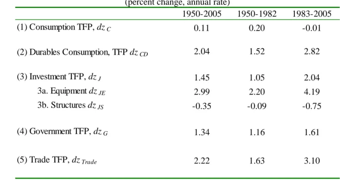
We first examine the long-run properties of the data from 1950 to 2005, which we also break into sub-periods of 1950-1982 and 1983-2005. Table 1 shows the sample-average growth rates of final-use TFP (the top panel) and technology (the bottom panel). Since utilization should be stationary in the long run, both TFP and utilization-adjusted TFP should have much the same means. This prediction holds in the data, with differences between the top and bottom panels showing up in the second or third decimal place. The data show the pattern we have come to expect, with the technology for producing equipment and durable consumption advancing at a rapid rate, on the order of 3 percent per year over the last two decades. The technology for producing non-durables and services (NDS) consumption improves very slowly over the whole period, and is essentially flat over the post-1983 period. The technology for producing structures shows a definite and puzzling decline over the whole period, which is particularly pronounced over the later period. We ascribe this decline to a lack of adequate adjustment for the increasing quality of structures in the official data. Similar mismeasurement probably also explains the lack of growth in NDS technology over the post-1983 period.19

Our mapping of industry production residuals to final-use categories also provides novel estimates of technology for two categories of output, government purchases and exports. Both have increased strongly over our sample period, particularly export technology, which grows at 2.1 percent from 1950 to 2005.

Figure 1 shows the ordering of growth rates visually by plotting the estimated levels of final-use technology (with utilization-adjusted residuals) that correspond to the bottom panel of Table 1. Note that our “government technology” is not the technology in the production of services by government workers, which are not included in our measure of output. Government technology

19

For example, the official statistics do not attempt, even in principle, to capture the gains from increased product variety.

growth captures improvement in the production technology for the goods that the government buys from private industries. The government purchases a mix of equipment, non-durables and services, and structures. Similarly, the correct interpretation of our “trade technology” is that it is the

technology for producing exports. Since exports are primarily goods (and about half durable goods), trade technology grows at a rate comparable to equipment technology and consumer durables.

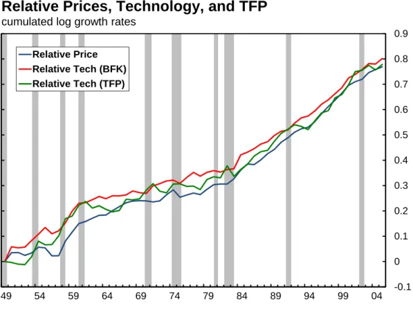
GHK and the literature building on their work use relative prices as a proxy for relative technology. Of course, under some assumptions this procedure is rigorously correct, but as discussed above these assumptions are restrictive. Now that we have an independent measure of sectoral technical change, derived under more general assumptions than GHK, we can ask an important question: To what extent do relative final-use output prices provide a good

approximation to relative final-use TFP or technology? Table 2 shows the comparison with

relative TFP (without utilization adjustments, so the identity derived in equation (4) holds exactly). As expected, the price of non-durables and services consumption has risen on average relative to the price of the equipment investment. This trend is more pronounced in the post-1982 period. Even so, relative prices do not change as fast as relative TFP. Table 2 shows that on average relative TFP has risen about 0.5 percent per year faster than the relative price. As discussed in the theory section, this can happen if there are differences in the growth rates of share-weighted primary input prices or long-run changes in the relative tax wedge. In fact, about two-thirds of the gap between relative prices and relative TFP is due to long-run changes in relative primary input prices, with the remaining gap due to changes in relative sales taxes. (The important factor for the tax wedge turns out to be rising sales taxes on consumer goods, which worked to raise consumer prices; the effect of tax changes on investment prices alone is relatively small.)

How can the growth rate of primary input prices diverge across sectors over a period of decades? One would think that prices for identical factors should equalize across industries over such long periods, and the composition corrections in the Jorgenson data should ensure that we are indeed comparing constant-quality inputs across sectors. (Thus, for example, if computer

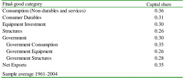
manufacturing requires a higher fraction of college-educated workers than auto manufacturing, we would not misinterpret this fact as implying that the price of homogeneous “labor” is higher in computers than in autos.) Recall, however, that the primary input prices are weighted by their cost shares. We know that over time the price of labor rises faster than capital rentals, so industries with high labor shares will, ceteris paribus, experience faster price growth. In Table 3 we report capital shares by final-use sectors, and show that this pattern does indeed hold in the data. That is, equipment investment does indeed have a lower capital share (and thus a higher labor share) than does NDS consumption. In addition to verifying the reason for the long-run gap between relative prices and relative TFP, the result that capital shares differ noticeably across sectors invalidates both short- and long-run identification based on uncovering relative technology change from the behavior of relative prices. Thus, the conclusions of a large literature are immediately called into question.production

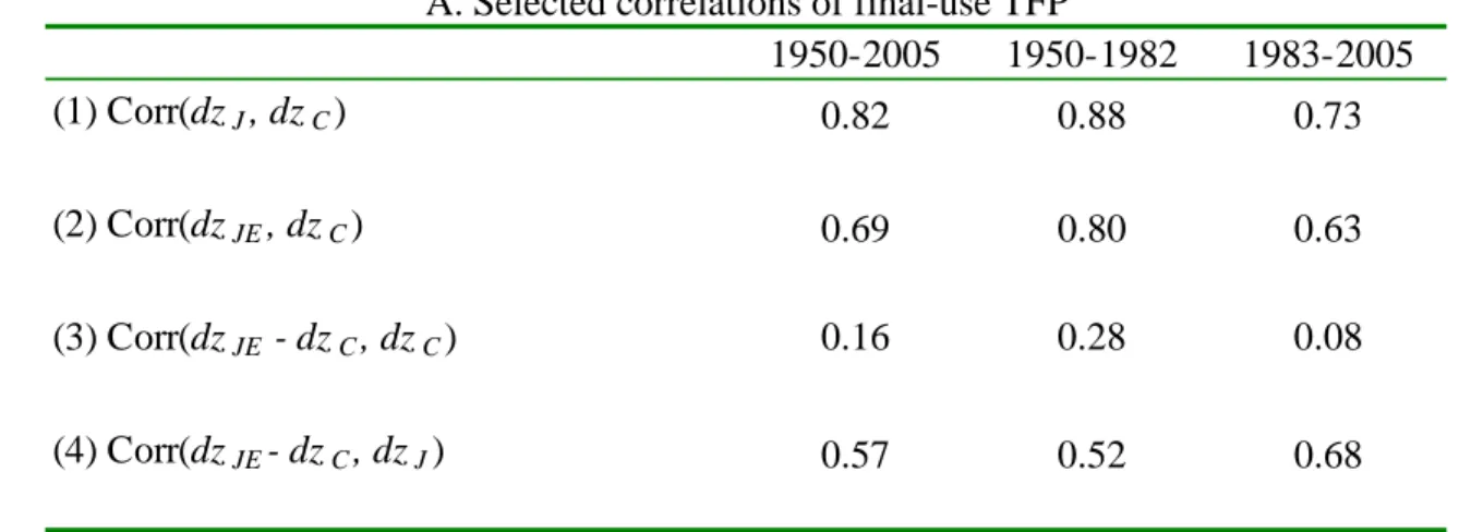
Tables 4A and 4B show selected correlations for standard TFP and BFK technology change, respectively.. The sectoral shocks themselves are very highly correlated, as shown in the first rows of each panel. This is not surprising: In addition to any truly “common” shocks, the final-sector shocks are different weighted averages of the same vector of underlying commodity shocks. However, the correlations are lower using utilization-adjusted TFP, as one expects: This control eliminates the common mismeasurement from business-cycle variations in factor

Our procedure allows us to test the orthogonality assumptions typically used in the preceding empirical literature. In particular, GHK and Fisher (2006) explicitly assume

orthogonality of what they label “neutral” and (equipment) “investment-specific” productivity innovations. In our two-sector framework, these labels correspond to the consumption-sector productivity shock and the relative equipment-investment-consumption shock. Line 3 of the two panels shows the correlation between the “neutral” and “equipment specific” shocks.

A priori, there seems little reason to expect orthogonality, given that these shocks are different mixtures of the same underlying productivity residuals. The orthogonality assumption appears shaky in the data, for both the standard and utilization-adjusted TFP series, where the correlations are about (plus or minus) 0.10. Note that Fisher (2006) does not assume that observed, standard TFP measures technology, so the utilization-adjusted result is probably more relevant. Note also that orthogonality with consumption TFP is a much better approximation than is orthogonality with investment TFP, as shown in line 4.20 However, whether or not the

orthogonality assumptions are verified, GHK’s and Fisher’s identification schemes cannot uncover relative technology from relative prices, since factor shares differ across sectors.

Finally, what are the dynamic effects of exogenous shocks to different types of technology? Table 5 shows dynamic responses of business-cycle variables to changes in sectoral technology. The first set of variables we study consists of GDP and its components, with all the dependent variables entered in growth rates.21 The table also shows the same regressions for other interesting macroeconomic variables: hours, wages, a variety of prices, and interest rates, with variables other

20

The correlations for the entire period are not the averages of the correlations for the subperiods, because the standard deviations over the entire period exceed the average of the standard deviations for the subperiods. An interesting question that we have not yet pursued is what orthogonality of relative TFP and consumption TFP implies about the input-output structure of the economy.

21

The GDP and investment data are taken directly from published BEA tables. They have not been adjusted using the Gordon investment deflators.

than interest rates entered in log differences. The R2 shown are for bandpass filtered data, i.e., where the dependent variable and the fitted values are first bandpass filtered to focus on variation between 2 and 8 years.

The challenge is the desire to be comprehensive in including all final-use shocks with the cost of using greater disaggregation (e.g., including structures separately), when multicollinearity becomes a serious problem. We aggregate final-use sectors in the way that corresponds to typical assumptions in two-sector models: One sector produces all investment goods, including equipment for both the private sector and the government, consumer durables, structures and exports; the other produces non-durables and services consumption for the household and government sectors. We group exports with investment goods, for two reasons. First, exports are mostly durable. Second, exports are a way of adding to a country’s durable wealth, just like equipment investment, for exports can be used to purchase capital held in the rest of the world. For all variables, we include the current value and two lags.

As the data section noted, we do face a problem in interpreting the terms of trade as exogenous. First, the terms of trade should change with changes in domestic consumption and investment technology, if these goods are exported. Second and more importantly, the terms of trade may change for reasons that are clearly not exogenous. For example, monetary policy can change the terms of trade if prices are sticky. Monetary policy may also react to changes in output or hours worked due to non-technology shocks, thus exacerbating the endogeneity problem.

We address this problem by constructing a second set of measures of technology that we do think are exogenous, using only industry technology shocks based on the utilization-adjusted TFP residuals. Operationally, we set to zero changes in the terms of trade as well as changes in the TFP of the natural resource industries and government enterprises. We then use this group of rigorously exogenous measures as instruments for the various types of technology change in Table 5.

Focusing first on the effects of investment-specific shocks, we find results similar to those documented by Gali (1999) and BFK (2006), which are puzzling from the standpoint of a simple one- or two-sector RBC model with flexible prices. Aggregate GDP, non-durables consumption, purchases of consumer durables, residential investment and imports all fall significantly after a positive shock to equipment technology. Most strikingly, equipment and software investment falls for two years after a positive shock to the technology for producing investment goods, and the decline is highly significant. This last finding is especially striking if one considers the likelihood of measurement error in our measures of investment output. Since we are regressing equipment growth on the technology for producing equipment, measurement error in output would create a positive bias in the coefficient. Adjusting for measurement error, the true coefficients are likely to be even more negative than our estimates. (There is little autocorrelation in the investment

technology growth series, so this result doesn’t seem to reflect predictability that equipment technology will be even better in the future. In some models, news of a future technology improvement will cause demand to contract until the improvement is actually realized.)

Table 5 shows that hours worked fall significantly when investment technology improves, and do not recover their pre-shock value even after three years. Note that this is a decline in total hours worked in response to a positive technology shock to a sector that (even with the inclusion of consumer durables) produces less than 20 percent of GDP! As shown in Table 6, the updated BFK results show a distinct and significant negative contemporaneous correlation between hours growth and aggregated BFK technology. (The negative effect is more pronounced with the original BFK industries, i.e., excluding agriculture, mining, and government enterprises).

As expected, an equipment-technology improvement does lower the relative price of equipment. Somewhat surprisingly, consumption prices also fall, as does the GDP deflator.

Next we examine the effects of consumption-technology shocks. Here again we find results at odds with simple RBC models which, as we noted, generally predict consumption technology neutrality. We see that consumption-technology shocks increase GDP and non-durables

consumption significantly, but also increase equipment investment, consumer durables consumption and (on impact but not cumulatively) residential housing, with at least one

statistically significant impact in each category. Hours worked are basically unchanged over the three years. As expected, the relative price of consumption to equipment falls, but the decline is not statistically significant.

The final column of Table 5 shows the R2 of the regression, after bandpass-filtering both the dependent variable and the fitted value in order to focus on business-cycle frequencies. For quantity variables, especially, the explanatory power is quite high. Figure 3 shows the fitted values of hours and equipment to technology shocks. The explanatory power of the regression is clear. Comparing the fitted values in the top and bottom panels, it is also clear that, conditional on technology, hours and equipment investment move comove positively. But it is also clear that, according to the regressions, technology innovations did not cause the deep recessions of the 1970s and 1980s.

Our simple model of Section II predicts that business investment should not change in response to a consumption technology improvement. The model did not include residential investment and consumer durables. We conjecture that if the model is extended to allow for durable goods to provide services that directly enter the utility function, and incorporates non-separability between non-durables consumption and durables services, it would predict roughly the results that we find, at least qualitatively,

Taken together, these results suggest that the earlier findings of Gali (1999) and BFK (2006) about the contractionary effects of technology improvements are driven primarily by the

effects of investment technology shocks. They also raise an interesting question: Does any fairly standard model predict that consumption technology improvements should be expansionary, but investment technology improvements should not? We believe that a simple two-sector model with sticky prices in both sectors and a standard Taylor rule for monetary policy can go some way towards matching the results we find. Preliminary results obtained by Basu, Fernald and Liu (2012) suggest that we are right.

A reason the sticky price model may be appropriate is the extremely slow pass-through of technology to relative prices. The pass-through was almost imperceptible in the regression results. However, other models of slow pass-through (for example, in flexible-price models with time-varying markups), might also explain the results we find.

Considering the results altogether, we find strong evidence that we cannot summarize technology shocks using a single aggregate index. Aggregation would hold either if (1) all final-use technology shocks were perfectly correlated or (2) if the different shocks had identical economic effects. Unfortunately, neither condition is satisfied, since Table 4B shows that the relevant correlation is about 0.50, and we can statistically reject the hypothesis that all the

coefficients of investment- and consumption-technology shock in Tables 5 are identical at all lags. Hence, it appears important to use multi-sector models to investigate economic fluctuations due to technology shocks.

Table 5 has some interesting findings that bear on the sticky-price interpretation of our results, and suggest some new thinking about optimal monetary policy. Note that the Fed Funds rate falls significantly and sharply in the first two years following a consumption technology improvement, but barely changes following an investment technology improvement.

Correspondingly, the GDP deflator falls for all three years following an investment shock, but only on impact and insignificantly following a consumption shock. If the Fed targets consumption

prices, but not investment prices, then that would go a long way towards explaining why the effects of an investment shock are so contractionary but the effects of the consumption shock are

expansionary. These results also suggest that optimal monetary policy should target investment as well as consumption goods prices.

VI. Conclusions

Theory suggests that the final-use sector in which technology shocks occur matters for the dynamic response of those shocks. We make this point with the example of

consumption-technology neutrality in the real-business-cycle model. Consistent with the predictions of the model, our empirical results show that consumption- and investment-specific shocks do indeed have significantly different economic effects, and the differences persist for at least several years.

The details of the results present several puzzles. The results for investment-sector shocks show that hours decline when investment technology improves, GDP declines sharply and, most surprisingly, investment itself declines strongly. These results are consistent with the findings of Gali (1999) and BFK (2006), who interpret them as evidence in favor of nominal price rigidities. Our findings for consumption shocks are quite different, however: they show significant increases in GDP and in the consumption of both non-durables and durable goods, including housing. Whether these results taken together can be explained by richer or differently-parameterized flexible-price or sticky-price models with multiple sectors is at this point an open question, although we find two-sector sticky price models promising in this regard.

A novel contribution of this paper is a new method to measure sector-specific technologies that does not rely simply on relative price changes, as frequently used in the macro literature. In special cases, the relative-price measures are appropriate; but in general, they are not. We show that the conditions necessary for relative prices to measure relative technologies do not hold in the

data. Since our method allows us to test hypotheses that are identifying assumptions in other works, it is a robust, albeit data-intensive, way of checking whether these assumptions hold in any situation where their validity is in doubt.

Appendix A: The Optimal Mode of Production

Closed Economy: Stretching terminology a bit, define “final” or “net” output of a commodity as the quantity produced that is used in the direct production of consumption,

investment, government purchases—that is, the amount not used in the production of intermediate goods. Gross output of a commodity is the total amount of the commodity produced for all purposes.

Let R be the rental rate for capital K, W the wage for labor N, and Z a vector of multiplicative technology shifters. Consider the cost minimizing plan for making one unit of final or net output of commodity i available for use in producing C, J, G:

(1.5) ˆ _,ˆ _,ˆ _,ˆ ˆ ˆ ( , , ) min ˆ ˆ . . 1 ˆ ˆ _{( )} ˆ ˆ ˆ ˆ ln( ) ln( ) ln( ) ln( ) ln( ) ( ), ij ij ij ij i ij ij K N X M j j ii i i ij i j ij j jK ij jN ij j ij P R W Z R K W N s t Y M Y M j i Y Z a K a N b M j                











The i subscript refers throughout to the fact that the program is intended to produce net output of commodity i. The hats on key variables are a reminder that the program is for one net unit of commodity i. ( ,P R W Z_i , ) is the minimum average (and marginal) cost of producing

commodity i. Kˆ_ijis the amount of capital used directly to produce commodity j in order to produce one net unit of commodity i. Nˆ_ij is the amount of labor used directly to produce commodity j in order to produce one net unit of commodity i. Yˆ_ij is the total gross amount of commodity j used to produce one net unit of commodity i. Mˆ_ijis the amount of commodity  used directly to produce commodity j in order to produce one net unit of commodity i. Z_jis the multiplicative technology shifter for producing commodity j. a_jKis capital’s share in the direct inputs to commodity j. a_jNis labor’s share in the direct inputs to commodity j. Finally, b_jis the share of commodity  in the direct inputs to commodity j. Our objective in this appendix is to find the boiled down production function for net output of commodity i as a function of the technology vector and the total capital and labor inputs used directly or indirectly to produce net output of commodity i. We will use Shephard’s Lemma (also called the derivative principle) to find capital’s share _i and labor’s share 1_i, and the corresponding method to find the elasticity _ij of net output with respect to each component Z_jof the technology vector Z. To be specific, by Shephard’s Lemma, capital’s share in the boiled-down net output production function is given by

(1.6) ( , , ), ( , , ) i i i P R W Z R P R W Z R    