Content from this work may be used under the terms of theCreative Commons Attribution 3.0 licence. Any further distribution
Wind turbine
C
p,maxand drivetrain-losses estimation
using Gaussian process machine learning
E Hart1, W E Leithead2, J Feuchtwang3
1 Wind and Marine Energy Systems CDT, University of Strathclyde, Glasgow, UK 2 Centre for Industrial Control, University of Strathclyde, Glasgow, UK
3 Institute for Energy and the Environment, University of Strathclyde, Glasgow, UK
E-mail: [email protected]
Abstract. In this paper it is shown that measured data in a wind turbine, available to the
controller, can be formulated into a polynomial regression problem in order to estimate the turbine’s maximum efficiency power coefficient, Cp
,max, and drivetrain losses, assuming the
latter can be well approximated as being linear. Gaussian process (GP) machine learning is used for the regression problem. These formulations are tested on data generated using the Supergen Exemplar 5 MW wind turbine model, with results indicating that this is a potential low cost method for detecting changes in aerodynamic efficiency and drivetrain losses. The GP approach is benchmarked against standard least-squares (LS) regression, with the GP shown to be the superior method in this case.
1. Introduction
As wind turbine assets grow in size and move further offshore, where access becomes more problematic and expensive, the need for increased reliability becomes even more pronounced. Therefore, there is a need for a diverse range of monitoring techniques with which faults and behavioural changes in wind turbines can be quickly detected and appropriate steps taken. Due to this, there have been a huge number of new measurement techniques developed in recent years, all with their associated costs. In this paper, rather than proposing a new measurement technique per se, we instead look at how existing data available to a wind turbine controller can be more fully utilised in order to try and detect changes in a turbine’s aerodynamic efficiency and drivetrain losses.
Changes in aerodynamic efficiency can either happen rapidly, for example via icing of the blades [1], or slowly, for example via blade degradation [2]. Changes in the mechanical losses in the drivetrain can be indicative of damage or an imminent failure. In all cases, prior warning of any changes, and the tracking of such changes over time, is desireable to inform operation and maintenance (O&M) for these wind turbines.
The proposed method uses Gaussian process machine learning to perform polynomial
regression on noisy data available to the wind turbine controller. As will be shown, this
Gaussian process machine learning has already seen a range of applications in wind energy, including forecasting [8], structural health monitoring [9], and nonlinear dynamics identification [10].
2. Control Regions
The control strategy for a wind turbine generally contains two distinct regions while operational. Let ‘rated wind speed’ be the wind speed at which the wind turbine reaches its rated power output. Then the two major control regions are ‘below rated’ and ‘above rated’ operation. In this work we consider variable speed, variable pitch (VSVP) machines which represent the vast majority of the currently operational turbines globally. For such a turbine, a typical design power curve is given in Figure 1.
5 10 15 20 25
Wind speed (m/s) 0
1 2 3 4 5 6
Power
(W)
106
[image:2.595.182.420.276.452.2](MW)
Figure 1. Typical design power curve for a VSVP wind turbine. The rated power here is 5
MW. Note, this is the power curve for the Supergen turbine model used to generate data for the current work.
The rated wind speed can be seen to be roughly 11.5 m/s. Above this point the turbine will be pitching in order to limit the power, while maintaining a constant rotational speed. This work, however, is focussed on the below rated portion of the power curve; where the turbine is attempting to maintain optimum efficiency in order to maximise power capture. This
corresponds to maintaining the tip-speed ratio, λ, defined as,
λ= ωrR
v , (1)
at the value which corresponds to maximum efficiency, this value will be denoted byλmax.
From Equation 1 it should be clear that maintaining λ =λmax requires the turbine rotational
the given turbine model. For a detailed explanation of how the turbine tracks the maximum efficiency curve see, for example, [4].
Rotor speed rad/s
0.7 0.8 0.9 1 1.1 1.2 1.3 1.4
Torque (Nm)
×106
0.5 1 1.5 2 2.5 3 3.5
Max eff. curve Op. strategy
99.5% of Cp
max eff. curves
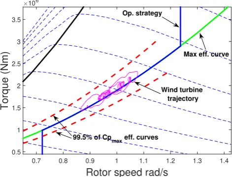
[image:3.595.173.409.162.342.2]Wind turbine trajectory
Figure 2. Wind turbine torque-speed diagram including maximum efficiency curve, design
operational strategy, 99.5% efficiency curves and a sample simulated trajectory of the wind turbine model. The dashed blue lines are constant wind speed curves and the solid black line indicates beginning of stall.
3. Deriving the Regression Equation
To recap, in below rated operation, and when away from transitional operating states, a wind turbine control system is attempting to track the maximum efficiency curve of the wind
turbine [6]. This corresponds to keeping the tip-speed ratio at λmax, the tip-speed ratio which
corresponds to Cp,max. No matter how sophisticated the control system, there will always be
some error when attempting to trackCp,max, with the true value of λvarying about λmax. For
example, this can be seen in the sample trajectory of Figure 2. Thus at each time step,
λ=λmax+ζλ, (2)
with error term ζλ. The aerodynamic torque, Qaer, is given by [3],
Qaer=
1
2ρARv
2CP(λ)
λ . (3)
Balancing torque terms gives that the above expression for aerodymanic torque will also be equal to,
Qaer=NQˆg+Jω˙ˆr+L(ˆωr), (4)
where the losses function L accounts for drivetrain torque losses; J is rotor inertia, Qaer and
Qg aerodynamic and generator torques respectively, ωr is generator speed and N the gearbox
ratio (the caret symbol is being used to indicate measured values). Manipulation of the
approximated as a polynomial regression equation involving Cp,max and the drivetrain losses;
ˆ
G := N1Qˆg+Jω˙ˆr
2ρAR3ωˆr2
(5)
(from Equations 3 and 4) = λ−3C
P(λ) +L∗(ˆωr) (6)
(Taylor exp. about λ=λmax) ≈ λ−max3 Cp,max+L∗(ˆωr) +δ, (7)
where L∗=−L/1
2ρAR 3ωˆ2
r and we have assumedζλ is small enough to allow us to approximate
the aerodynamic term λ−3CP(λ) (via a first order Taylor expansion about λ=λ
max) as being
the constant λ−3
maxCp,max plus an error term δ = mζλ with m = dλd λ−3CP(λ)
λ=λmax
. It is
further assumed that ζλ, and hence δ, is a noise term. Letting Φ denote the constant term
λ−3
maxCp,max, our measured data is then of the form,
ˆ
G= Φ +L∗(ˆω
r) +δ. (8)
Assuming torque losses increase linearly with rotational speed (torque losses have been shown to increase with what is essentially linear behaviour in the literature, for example see the loss
versus rotational speed diagrams in [5]) it follows that L∗ is quadratic in ˆω−1
r (with no constant
term).
Identification of Φ andL∗ in this case then allows for the losses, L, and the value of Cp,max
to be estimated and hence the identification of these terms has been formed into a polynomial regression problem, with all required data coming from information which is available to a wind
turbine controller. In order to form the regression measurements ˆG for a given wind turbine it
follows, from Equation 5, that the required data is: torque demand, rotational speed, gearbox ratio, rotor inertia and rotor radius.
4. Gaussian Processes
Gaussian process machine learning was initially developed in the early nineties after GPs were found to be the natural limit of some types of neural networks as the number of nodes tended towards infinity [7]. Modelling a function as a GP involves building multivariate Gaussian distributions between all possible subsets of function outputs across the functional domain [11].
Assuming a prior mean of zero, this amounts to determining a prior covariance function, k,
between any two outputs of the given function. Covariances between a function’s outputs are generally modelled as being a function of the input variables for each pair of output points [11].
Thus for a function, f(x) say, being modelled as a zero prior mean GP then the covariance
between function valuesf(x1) and f(x2) will be modelled as,
cov(f(x1), f(x2)) =k(x1, x2), (9)
for some covariance function k.
Probably the most commonly used covariance function is thesquared-exponential covariance
function,
k(x1, x2) =aexp
−d
2(x1−x2)
2
. (10)
Note that the parameters a and d determine the amplitude and lengthscale of the covariance
function respectively.
the correct covariance function. A polynomial covariance function can be readily derived by assuming that the polynomial coefficients are zero mean, independent random variables, this
results in the covariance function shown in Equation 11 [12], wheredis the degree the polynomial
and the parameters γk are the variances of the corresponding polynomial coefficients.
kP(x1, x2) = d X
k=0
γkxk1xk2. (11)
The γk parameters are determined prior to making predictions using the measured regression
data in a standard maximum-likelihood optimisation procedure [11], the measured data is
assumed to be corrupted by independent Gaussian noise and the variance, ξ, of this noise is
determined in this same optimisation procedure.
Once this GP prior has been determined, regression is performed by conditioning the prior on the measurements via the Gaussian conditional distribution [11, 12].
5. Simulation and Data Collection
The above derivations have been investigated using simulated data from the Supergen Exemplar 5MW wind turbine model, full details of which can be found in [6]. Summary data for this model is given in Table 1. Both the power curve and torque-speed diagrams, along with the sample trajectory, in Figures 1 and 2 were produced using this model. Simulations were run over a range of wind conditions with mean wind speeds between 5 and 8 m/s, turbulence intensities of between 5 and 20% and a power law shear exponent of 0.2. The relevant data, i.e. that
required to determine ˆGin Equation 5, was extracted from the model. The turbine simulations
[image:5.595.170.432.479.589.2]were performed in Simulink software and then GP regression and results analysis was done using Matlab.
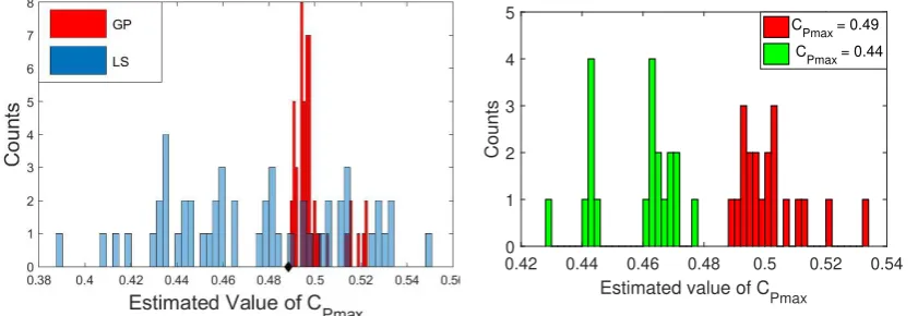
Table 1. Data for simulated wind turbine.
Rated power 5 MW
Rotor diameter 126 m
Blade number 3
Hub height 90 m
Aerodynamic control Pitch
Fixed/Variable speed Variable
Pitch Controller PI with low pass filter
Below Rated Torque Control Closed loop
As can be seen in the sample trajectory of Figure 2, correlations exists for short time-scales
in the turbine measurements. Autocorrelation investigations of the measured values, ˆG, have
shown 20s to be a suitable sampling time in order to avoid having correlated measurements for the current model. Hence, data points were extracted at intervals of 20s during simulation.
Polynomial regression was then performed on these measured values using GP machine learning. For the current case we are performing a quadratic polynomial regression, hence the GP covariance function is,
kP(x1, x2) =γ2x21x 2
2+γ1x1x2+γ0. (12)
In order to provide a benchmark, standard least-squares (LS) polynomial regression is also
regression techniques were extracted the given estimates of theCp,maxvalue and drivetrain-losses
function. This is done by scaling the given coefficients by the appropriate terms, for example, in
order to obtain theCp,maxestimate from the constant coefficient Φ, as determined by regression,
one simply multiplies byλ3
max.
6. Results
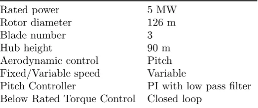
This regression problems was found to require a robust (in the statistical sense) method for its solution. This is due to the characteristics of the measured data which have been found to contain outliers, has heavy tails and the noise term present is strongly non-Gaussian; all factors which make finding accurate solutions more difficult. Figures 3 and 5 show the values
ofCp,maxand the drivetrain loss functions respectively predicted by both LS and GP regression
techniques. Each prediction is from a dataset containing 500 points, corresponding to roughly 3 hours of realtime operation.
Figure 3. Cp,max estimates from both GP
and LS. The true value is given by the black diamond.
0.42 0.44 0.46 0.48 0.5 0.52 0.54
Estimated value of C
Pmax 0
1 2 3 4 5
Counts
C
[image:6.595.97.518.309.454.2]Pmax = 0.49 CPmax = 0.44
Figure 4. Cp,max estimates from datasets
with two different values of maximum efficiency.
In Figure 3 it is clear that the GP approach is superior to using LS. While the GP predictions
are clustered close to the true value of Cp,max, with some amount of positive bias, the LS results
on the other hand are spread almost uniformly across the range of probable values. Based on
the GP clustering, one would expect a shift inCp,maxby some small amount to be detectable. In
order to test this hypothesis, regression was performed on a dataset generated with allCpvalues
reduced by 0.05 and compared to regression on the original data. Cp,max estimates from these
two cases are shown in Figure 4 where the sets of prediction clusters are clearly separate, and hence the GP predictions are indeed able to detect this shift in aerodynamic efficiency. Note that the positive bias in the GP predictions appears to be from the noise distribution being non-symmetrical.
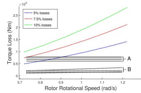
Similar results are then observed for the drivetrain loss predictions in Figure 5 where the true losses in the model are shown along with various GP and LS regression predictions. Again, the GP predictions are much more tightly clustered and, while they do show a bias, GP regression here can be seen to give both more accurate and more consistent predictions of the losses in the drivetrain.
Rotor Rotational Speed (rad/s)
0.7 0.8 0.9 1 1.1 1.2 1.3
Torque Loss (Nm)
×105
-4 -3 -2 -1 0 1 2 3
5% losses 7.5% losses 10% losses True losses
}- GP
[image:7.595.86.311.114.288.2]}- LS
Figure 5. Drivetrain loss predictions along with loss contours (percentages in terms of design power values at each rotational speed).
Rotor Rotational Speed (rad/s)
0.7 0.8 0.9 1 1.1 1.2
Torque Loss (Nm)
×105
0 0.5 1 1.5 2
2.5 5% losses
7.5% losses 10% losses
}- A
[image:7.595.311.553.131.290.2]}- B
Figure 6. Drivetrain loss predictions along with loss contours for two different loss function cases.
obtained by shifting the left hand value of the original loss function down by 2.5%. This second set of predictions is labelled cluster B. It can be seen that these two clusters are clearly separate and so this shift in losses is detectable when using the GP regression approach.
7. Discussion
The results presented here first demonstrate that GP is superior to LS in this case, with LS results being so scattered as to make them effectively useless. The GP results, while more tightly clustered, do suffer from a bias which appears to be due to assymetrical noise being present. However, as discussed in Section 1, the identification of a turbine’s maximum efficiency coefficient and drivetrain losses in below rated operation is being developed primarily for turbine monitoring
and O&M purposes; for this type of application it is the ability to detectchanges in these values,
rather than the exact values themselves, which is key to forewarning of potential issues. Hence, for the desired application these offsets do not pose a significant problem. Nevertheless, in future
work attempts to remove these biases will be made, focussing on the λ terms which will vary
asymmetrically with wind speed and hence may be a strong source of bias here. If this is found to be the case then it may be possible to reformulate the regression problem in order to account for the bias term.
When considering GP predictions of bothCp,max and drivetrain losses, the current work has
demonstrated that GP regression is sensitive enough to detect changes in these values. The next stage in developing this method will therefore be to devise an automated strategy for determining when perceived changes in predictions are deemed to be significant. This will most likely be done by implementing the probabilistic aspects of GP models in order to give confidence intervals for the predictions and so probabilistic thresholds can be used to indicate when a likely shift in value has been detected.
8. Conclusions
The identification of a wind turbine’s Cp,max value and drivetrain-losses was formulated as
useful and inexpensive tool for detecting changes in wind turbine dynamics for monitoring and O&M purposes. This method is also attractive because it does not require any new sensors to be installed, since all required data is already available to the wind turbine controller. Future work on this method will focus on removing the prediction biases and validating the results seen here using real turbine data.
References
[1] Wang X, Bibeau E, and Naterer G 2007Experimental investigation of energy losses due to icing of a wind turbine, International Conference on Power Engineering, Hangzhou, China
[2] Sareen A, Sapre C and Selig M 2014Effects of leading edge erosion on wind turbine blade performance, Wind Energ. 17:15311542
[3] Burton T, Jenkins N, Sharpe D and Bossanyi E 2011 The Wind Energy Handbook, Second Edition, John Wiley & Sons
[4] Bianchi F, Battista H and Mantz R 2007 Wind Turbine Control Systems, Advances in Industrial Control, Springer-Verlag London
[5] Martins R, Fernandes C, Seabra J 2015Evaluation of bearing, gears and gearboxes performance with different wind turbine gear oils, Friction 3(4): 275286
[6] Stock A 2016, Augmented control for flexible operation of wind turbines, PhD Thesis, EEE, University of Strathclyde, Glasgow
[7] Neil R 1994Priors for infinte networks, Technical Report CRG-TR-94-1, University of Toronto, Canada [8] Chen N, Qian Z, Nabney I and Meng X 2014Wind power forecasts using gaussian processes and numerical
weather prediction, IEEE Trans. Pow. Sys. 29-2
[9] Papatheou E, Dervilis N, Maguire E and Worden K 2014 Wind turbine structural health monitoring: a short investigation based on SCADA data, 7th European Workshop on Structural Health Monitoring, Jul 2014 [10] Seng K 2008, Non-Linear Dynamics Identification Using Gaussian Process Prior Models Within a Bayesian
Context, PhD Thesis, Hamilton Institute, National University of Ireland
[11] Rasmussen C E and Williams C 2006,Gaussian Processes for Machine Learning, MIT Press