Convolution-based classification of audio and symbolic representations of music

City, University of London Institutional Repository

Citation

:

10.1080/09298215.2018.1458885

This is the accepted version of the paper.

This version of the publication may differ from the final published

version.

Permanent repository link: http://openaccess.city.ac.uk/id/eprint/19768/

Link to published version

:

Copyright and reuse:

City Research Online aims to make research

outputs of City, University of London available to a wider audience.

Copyright and Moral Rights remain with the author(s) and/or copyright

holders. URLs from City Research Online may be freely distributed and

linked to.

City Research Online: http://openaccess.city.ac.uk/ [email protected]

Convolution-based Classification of Audio and Symbolic

Representations of Music

Gissel Velarde∗1_{, Carlos Cancino Chac´on}2_{, David Meredith}1_{, Tillman Weyde}3 _{and Maarten}

Grachten2

1_{Aalborg University, Denmark}

2_{The Austrian Research Institute for Artificial Intelligence, Austria} 3_{City, University of London, United Kingdom}

Abstract

We present a novel convolution-based method for classification of audio and symbolic

repre-sentations of music, which we apply to classification of music by style. Pieces of music are first

sampled to pitch–time representations (spectrograms or piano-rolls), and then convolved with a

Gaussian filter, before being classified by a support vector machine or by k-nearest neighbours

in an ensemble of classifiers. On the well-studied task of discriminating between string quartet

movements by Haydn and Mozart we obtain accuracies that equal the state of the art on two

datasets. However, in multi-class composer identification, methods specialized for classifying

symbolic representations of music are more effective. We also performed experiments on

sym-bolic representations, synthetic audio and two different recordings ofThe Well-Tempered Clavier

by J. S. Bach to study the method’s capacity to distinguish preludes from fugues. Our

experi-mental results show that our approach performs similarly on symbolic representations, synthetic

audio and audio recordings, setting our method apart from most previous studies that have been

designed for use with either audio or symbolic data, but not both.

Index terms—Classification algorithms, composer classification, genre classification, convolution, filtering, audio music classification, symbolic music classification

∗

Correspondence: Gissel Velarde, Aalborg University, Department of Architecture, Design and Media Technology, Rendsburggade 14, Building: 6-314, 9000 Aalborg, Denmark. Email: [email protected]

1

Introduction

Methods modelling style recognition are of interest in music information retrieval for their ap-plicability in, e.g., music indexing, recommendation systems, and music generation, as well as in systematic musicology where they can foster the understanding of music. From the computational perspective taken in this study, style can be seen as a set of distinctive features shared among the instances of a style. Perceptually, style is a phenomenon that lets us characterize artists, genres, periods of composition, etc., on the basis of distinguishing salient features of works, despite variation or evolution over time (Paul & Kaufman, 2014; Rush & Sabers, 1981).

Most methods for classifying musical works have been specialized for use with either symbolic representations or digital audio files, but not both; and considerably more effort has been devoted to classification of music audio data. Most work in the audio domain builds models of timbre and instrumentation (Sturm, 2014b), while approaches in the symbolic domain are based on higher level musical descriptors derived from pitch–time structure.

The motivation for developing a method that can be applied in both domains stems from the successful use of visual representations of music in classification (Costa, Oliveira, Koerich, Gouyon, & Martins, 2012; Lidy & Schindler, 2016; Velarde, Weyde, Cancino Chac´on, Meredith, & Grachten, 2016; Wu et al., 2011) and the fact that both audio and symbolic music representations can be cast as images on a pitch–time plane. Spectrograms resemble noisy piano-roll representations, so intuitively one would think that a method that works well on a piano-roll representation might also work on a spectrogram. We expect some musical features to be useful for style recognition independently of representation (symbolic or audio), at least for music where timbral features are not required to distinguish a style. Having a single method that works equally well on both audio and symbolic data is interesting if one wants to index large heterogeneous multimedia music collections containing both score encodings and recordings, see for example the International Music Score Library Project (www.imslp.org) or the databases of IRCAM (http://ressources.ircam.fr).

3

computational methods proposed to date for discriminating between these two composers have been applied to symbolic representations of music, with accuracies above self-declared experts (Herlands, Der, Greenberg, & Levin, 2014; Hillewaere, Manderick, & Conklin, 2010; Hontanilla, P´erez-Sancho, & I˜nesta, 2013; van Kranenburg & Backer, 2004; Velarde et al., 2016). Most of these methods rely on features designed by experts, making them less general, and/or require each part or voice to be encoded separately. An exception is the model proposed by Velarde et al. (2016), which is based on classifying music from two-dimensional representations such as piano-rolls.

The method proposed by Velarde et al. (2016) learns to discriminate between classes of music by using filtered images of piano-roll excerpts to predict class labels, exploiting the images’ textures. However, local structures on the level of motifs prove to be very important in melodic similar-ity (van Kranenburg, Volk, & Wiering, 2013), and melodic segmentation using small time-scales has been shown to improve recognition in parent work identification (Velarde, Weyde, & Meredith, 2013). We hypothesize that style recognition requires the use of both large- and small-scale feature extraction mechanisms. Locality is desired to detect musical patterns even if translated in time and pitch. Therefore, in this study we extend the method of Velarde et al. (2016), introducing music segmentation, and test the effect of chunking pitch–time representations into small segments for classification. In this context, motifs are patterns at the level of a few notes—typically less than a bar. Local regularities in the form of reused patterns or motifs may be found by comparing segments at below the bar level. Finally, we experiment with combining classification strategies in ensembles.

In this paper we make the following contributions:

• We report experimental results matching state-of-the-art composer-identification results on

two different datasets of the Haydn and Mozart string quartets. We also report classification accuracies on multi-class composer recognition.

• We propose a new classification method which performs similarly well on both audio recordings

and symbolic representations of music.

• We report results of an experiment on discriminating between preludes and fugues from The Well-Tempered Clavier by J. S. Bach.

review of convolutional mechanisms. In section 2, we present the method and in section 3, we show the results of our experiments on composer recognition and genre classification. In section 4 we discuss our findings and we present our conclusions in section 5.

1.1 Computational approaches to music classification

There are only a few classification methods that have been designed for and evaluated on audioand

symbolic representations of music. For example, Tzanetakis, Ermolinskyi, and Cook (2003) demon-strated the use of pitch histograms for genre classification in both domains (audio and symbolic); and Cataltepe, Yaslan, and Sonmez (2007) and Lidy, Rauber, Pertusa, and I˜nesta (2007) combined symbolic and audio features to improve their classifiers on genre recognition. The classification accuracies reported by Tzanetakis et al. (2003) on a dataset containing electronica, classical, jazz, Irish folk and rock music, reached 50±7% on symbolic representations, 43±7% on synthetic audio, and 40±6% on recorded audio files. The classification accuracies reported by Lidy et al. (2007) on a dataset containing classical, pop and jazz music, reached 75% on symbolic representations, 86% on synthetic audio, and 93% when symbolic and synthetic audio representations were used in com-bination. While the approach by Cataltepe et al. (2007) seems to be more accurate using symbolic representations, the method by Lidy et al. (2007) works better on audio. Genres like classical, pop and jazz music typically use sets of instruments, and therefore, the use of timbre features appears to be relevant in the method by Lidy et al. (2007).

5

The second method evaluated at the MIREX (Lidy & Schindler, 2016), transforms the input to MFCC images, and aims to learn temporal and timbral features by means of a parallel single layer convolutional neural network. The classification accuracy obtained by this method on classical composer and latin genre classification reached 67.6% and 69.5% respectively.1 Both methods use a combined strategy of image processing and timbre feature extraction.

In the symbolic domain, most computational methods rely on the separate encoding of each part or voice, and in most cases use a predefined set of musical features (e.g., contrapuntal characteristics) before applying ak-Nearest Neighbour algorithm (k-NN), an SVM,n−grams, neural networks or Bayesian classifiers (Herlands et al., 2014; Hillewaere et al., 2010; Hontanilla et al., 2013; Ogihara & Li, 2008; van Kranenburg & Backer, 2004). On recognizing works by Bach, Handel, Telemann, Haydn and Mozart, van Kranenburg and Backer (2004) report a classification accuracy of 80.1%, with a method based on style markers and k-NN classification. Hontanilla et al. (2013) report an accuracy of 78.8% based on a 4-gram model on the same dataset. In this context we aimed to design a method that does not require hand-coded feature extraction and is applicable to audio and symbolic data.

1.2 Convolution mechanisms

It is well established that filtering (and convolution in particular) is ubiquitous in the perceptual systems of animals (Snowden, Thompson, & Troscianko, 2012). Local processing aspects of visual perception can be effectively described as a form of filtering or convolution (Murdock Jr., 1979; Pribram, 1986). In experiments involving functional neuroimaging, Gabor filters have been used to identify natural images from activity in the visual cortex (Kay, Naselaris, Prenger, & Gallant, 2008). Audition has been modeled with bandpass filters (Daubechies & Maes, 1996; Karmakar, Kumar, & Patney, 2011). Machine learning approaches use filtering combined with SVMs or neural networks for image classification tasks (Bengio, Courville, & Vincent, 2013; LeCun, Kavukcuoglu, & Farabet, 2010; Tuia, Volpi, Mura, Rakotomamonjy, & Flamary, 2014). These techniques help to enhance the relationships between pixels in the image, e.g. by highlighting edges or smoothing out local varia-tions. In music classification, filtering has been shown to significantly improve recognition (Velarde et al., 2016).

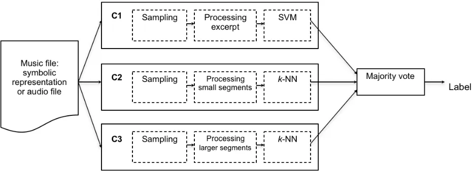
Figure 1: Diagram of the proposed method for music classification of symbolic or audio representations. The method receives a piece of music and outputs its computed class label. This method consists of an ensemble of three classifiers denoted by C1, C2 and C3, more specifically C1A, C2A and C3A for audio and C1S, C2S and C3S for symbolic music representation. Details on the configurations for each classifier are given in Table 1.

2

Method

An overview of the proposed method is presented in the diagram in Figure 1. The system receives a piece of music as input and computes its class label as output. It consists of an ensemble of three classifiers, denoted by C1, C2 and C3. We use classifiers with audio-specific input processing, henceforth denoted by C1A, C2A and C3A, or classifiers for symbolic music representations, denoted by C1S, C2S and C3S. Each classifier consists of a sampling, a processing and a classification phase. The predictions of the three classifiers are combined by majority vote (Kuncheva, 2004) to predict the final class label. In the multi-class case, if each classifier votes for a different class, the class assigned is the one whose numeric label is least.

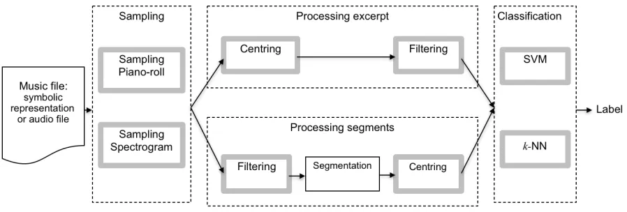
Figure 2 shows in more detail the possible configurations of the individual classifiers. In each classifier, a piece of music is first sampled to a two dimensional (2D) piano-roll image if the input is a symbolic representation of music (e.g., MIDI file), or to a 2D magnitude spectrogram image if the input is an audio file (e.g., WAV file). After sampling this 2D image, either theprocessing excerpt

or theprocessing segments phase follows. The main difference between the two processing phases is their output: the processing excerpt phase has one output per piece, while theprocessing segments

7

Figure 2: Diagram of the possible configurations of individual classifiers. An individual classifier receives a piece of music, which is first sampled, processed and finally classified. Modules represented by boxes with thick grey borders are optional processing steps. In thesampling andclassificationphases, vertically aligned boxes are exclusive processing steps, such that only one module can be activated. A piece is either processed in processing excerpt or in processing segments. In theprocessing excerpt phase both modules are optional, while in theprocessing segments phase, thesegmentation module is always activated.

onsets, while segments correspond to shorter units of about 1 to 2 quarter notes. Finally, there is a

classification phase employing an SVM or ak-NN algorithm. For pieces that follow the processing segments phase, the class label of a piece of music is the most frequently predicted class of its segments. Modules represented in Figure 2 by boxes with thick grey borders are optional processing steps. Details of each phase are given below.

2.1 Sampling

A symbolic music encoding format is one that provides information similar to that given in a score and in which the atomic component is typically a note; whereas a PCM audio file represents the sound of a specific performance of a piece in terms of a sampled waveform. The sampling phase prepares the input so that music is similarly represented as a 2D pitch–time representation regardless of whether it is a symbolic encoding or an audio recording. Symbolic representations of music are sampled to piano-roll images, while audio files are transformed into spectrograms.

2.1.1 Piano-rolls

of such an image by P and its width by T. The piano-rolls are sampled using each note’s pitch, onset, and duration. Onset and duration are encoded in quarter notes (qn). Chromatic pitch is represented by MIDI Note Number (MNN). MNN represents pitch as integer numbers from 0 to 127, C4 is mapped to MNN 60. Alternatively, pitch is encoded as morphetic pitch (Meredith, 2006, p. 127), which is a function only of the vertical position of the note-head of a note on a staff and the clef in operation on the staff at the position where the note occurs. We compute morphetic pitch from MIDI files using a pitch spelling algorithm called PS13s1 that requires parameters for defining a context window around the note to be spelt (Meredith, 2006). Thepre-context parameter is set to 10 notes and post-context is set to 42 notes, as these values performed best in Meredith’s (2006) evaluation using a dataset of baroque and classical music, the type of music used in this study. Morphetic pitch intervals are invariant to transposition within the scale, while chromatic pitch intervals are not (cf. Velarde et al., 2016). The sampling rate for piano-rolls of full-length pieces, denotedpf l, is 8 samples (i.e., pixels) per qn. Piano-rolls denoted byp400nrepresent the first

400 notes of each piece. p400n piano-rolls are first sampled with a sampling rate of 8 samples per

qn and then resized by nearest-neighbour interpolation (de Boor, 1978) to reach the size of P×T

pixels. In this case, the sampling rate might vary for each image.

2.1.2 Spectrograms

Spectrograms are used to present spectral information over time and have previously been used successfully for music classification (Costa et al., 2012; Wu et al., 2011). We use 2D greyscale images of spectrograms, generated from mono audio signals. Spectrograms are images of sizeP×T

pixels taking values from the interval [0,1]. The audio signals we use are either recordings of human performances or synthesized from symbolic representations. The synthetic audio files are generated from the first 400 notes of each piece encoded in symbolic format, using either a horn sound or a string sound. The horn and string sounds were approximated by frequency modulation synthesis and sample-based synthesis, respectively.2 The horn and string sounds were sampled at 22.05kHz

2

9

and 44.1kHz, respectively. The audio recordings correspond to excerpts of 30 seconds. The stereo recordings are converted to mono by taking the average of the left and right channels.

Spectrograms are obtained using the short-time Fourier transform (STFT) or the variable-Q transform (VQT) (Sch¨orkhuber, Klapuri, Holighaus, & D¨orfler, 2014).3 STFT spectrograms are computed with a Hamming window of size 1024 samples and 50% overlap, as in (Wu et al., 2011). VQT spectrograms are computed with 48 frequency bins per octave and the parameter γ = 20, which is used to increase the time resolution in the lower frequency range (Sch¨orkhuber et al., 2014).

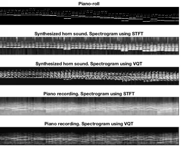
Figure 3 shows examples of the types of pitch–time representation that we use, including a piano-roll sampled from an excerpt of a MIDI file, along with spectrograms of recorded and synthesized audio. As the MNN is logarithmic with respect to frequency, both STFT and VQT spectrograms are plotted with a logarithmic scale for frequency.

2.1.3 Size of images

The piano-roll images of excerpts p400n are all 56×560 pixels. The size of piano-rolls of

full-length pieces (pf l) varies along the time axis according to the length of each piece. In audio,

we use only spectrograms of excerpts of music, denoted by sp400n. Due to the spectral content

in spectrograms, we use a higher resolution than piano-rolls, i.e., 150 pixels on the pitch axis. To approximately preserve the same amount of information as piano-rolls, we reduce the temporal resolution of spectrograms, downsampling them to 200 pixels, such that all spectrograms have a size of 150×200 pixels. STFT spectrograms were downsampled from 344×398 pixels to 150×200 pixels using bicubic interpolation (Keys, 1981). VQT spectrograms were generated using the resolution of 150×200 pixels.

2.2 Processing phase

Once the piece is sampled, it can be processed as an excerpt or as segments as seen in Figure 2. Only one of the two processing phases is used in any one classifier. The input for the processing phases is a 2D pitch–time image of size P ×T, either a piano-roll or a spectrogram as described above.

3

11

2.2.1 Processing excerpt

The processing excerpt phase has two modules, first centring (2.2.2.3) and then filtering (2.2.2.1), see Figure 2. Each of these two modules can be activated or deactivated in a configuration. All pitch–time images entering this phase have the same input size of P ×T pixels, and correspond to excerpts of music consisting of either the first 400 notes of a piece, if the input is symbolic or synthesized representations, or excerpts of 30 seconds in the case of audio recordings.

2.2.2 Processing segments

Theprocessing segments phase uses three modules in the following order: filtering (2.2.2.1), segmen-tation (2.2.2.2) and centring (2.2.2.3) as seen in Figure 2. Unlike the processing excerpt phase, the segmentation module is always active in this processing phase. If thecentring module is active, each segment is centred individually. The processing segments phase outputs several segments, which are sent to the classification phase (2.3).

2.2.2.1 Filtering

For the filtering module of the processing phase, we convolve pitch–time images with a rotationally symmetric Gaussian filterg:

g(x, y) =e

−(x2+y2)

2σ2 ₍₁₎

where (x, y) is the position of a point. We use a Gaussian filter of size 9×9 pixels and the standard deviation of the Gaussian distribution σ = 3 (as in Velarde et al., 2016). This filter is relatively small to keep the blurring localised.

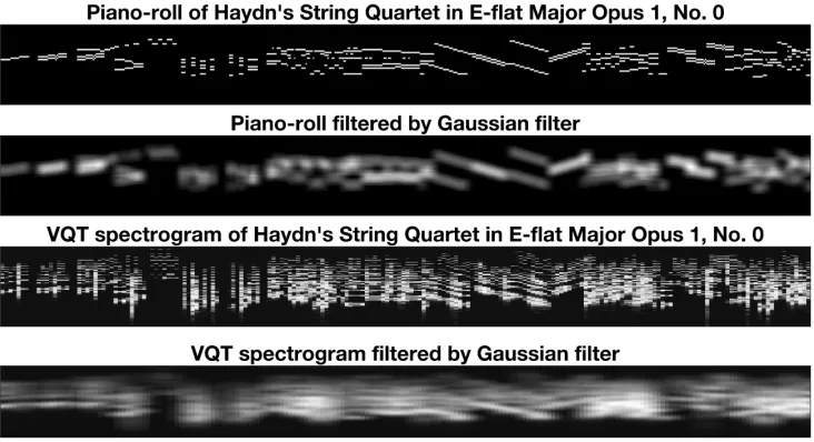
Figure 4: Excerpt of Haydn’s String Quartet in E-flat Major Opus 1, No. 0, in four pitch–time representations, from the top to the bottom: Piano-roll (p400n) morphetic pitch representation, followed by its convolution

with a Gaussian filter (second image), VQT spectrogram of the same excerpt synthesized with a horn sound (third image), and finally the filtered version of the VQT spectrogram (fourth image).

2.2.2.2 Segmentation

We introduce asegmentationphase, as local processing has been found to be important in modelling melodic similarity for music classification (van Kranenburg et al., 2013; Velarde et al., 2013). We use constant-length segmentation, which chunks each image into segments of equal length. Given a pitch–time image of size P ×T pixels, this image is segmented along the time dimension into segments with a constant length of Lpixels into segments of sizeP×Lpixels. IfT modL6= 0, the width of the last segment is padded on the left to reach width L. Letn =dT /Le. Depending on the amount of overlap between the paddednth segment and the (n−1)th segment, we replace the (n−1)th segment with the nth segment using the following procedure: if T modL 6 0.3L, then thenth segment replaces the (n−1)th segment.

2.2.2.3 Centring

13

2.3 Classification

The input to the classification phase can be one sample if it comes from the processing excerpt

phase, or several samples (processed segments) if they come from theprocessing segments phase. In the latter case, the predicted class label of a piece of music is the most frequently predicted class of its segments. In theclassification phase we restricted ourselves to using an SVM ork-NN as shown in Figure 2. Other classification algorithms could be used, too, such as decision trees or logistic regression.

We train SVMs with the one-versus-one coding design, based on error-correcting output codes (All-wein, Schapire, & Singer, 2000). We use linear kernels with Sequential Minimal Optimization (SMO) and Karush–Kuhn–Tucker conditions set to 0.001, with samples normalized around the mean, and scaled to have unit standard deviation.

Thek-NN classifier is used with Euclidean distance and the next nearest point to break ties. The Davies and Bouldin (1979) criterion is used to select the numberk with the smallest dispersion of clusters and the centroids’ distances, from a set of odd numbers in the range 3 to 21. k-means cluster-ing is applied to segments with squared Euclidean distance and the k-means++ algorithm (Arthur & Vassilvitskii, 2007) for cluster centre initialization. If a cluster loses all its member observations, a new cluster is created from the furthest point from its centroid. The maximum number of iterations is set to 100.

2.4 The ensemble of classifiers

In the design of the ensemble, our goal is to have the same structure of individual classifiers for audio and symbolic representations: one classifier extracting features at large scale (C1), and two classifiers extracting local features at two small time scales (C2 and C3), as seen in Figure 1. Correspondingly, C1A, C2A and C3A are used for audio. We use different configurations for each classifier expecting to have diversity in their predictions when ensembled. Details on the configurations of each classifier are given in Table 1.

Classifier Representation Sampling Processing Filter Centring Classification C1S p400n Morphetic Excerpt Gaussian No SVM

C2S pf l or p400n Morphetic

Segments,

L= 8 pixels Gaussian Pitch range

k-NN

C3S pf l or p400n MNN

Segments,

L= 16 pixels Gaussian No

k-NN

C1A sp400 or sp30s VQT Excerpt Gaussian No SVM

C2A sp400 or sp30s STFT

Segments,

L= 4 pixels Gaussian No

k-NN

C3A sp400 or sp30s STFT

Segments,

L= 8 pixels Gaussian No

k-NN

Table 1: Details of the configurations of individual classifiers. Classifiers C1S, C2S and C3S are used for symbolic representations of music. C1A, C2A and C3A are used for audio files.

not obtain results for using different values of k in our k-NN classifier when using the processing excerpt phase. We intend to explore this in future work.

For symbolic representations we used morphetic pitch or MNN, while in audio, morphetic encod-ing would have required the system to have some kind of transcription module, which we avoided. Instead, we used two sampling methods VQT and STFT. As the time dimension of spectrograms was downsampled to almost half the size of the piano-roll time dimension, the segment length of C2A is half that in C2S. The same holds for classifiers C3A and C3S. None of the classifiers used for audio included centring when processing because of performance reasons. We used centring for classifier C2S, but not for C2A as it had a negative effect on its performance. In piano-rolls, the top and bottom regions are very uniform (mostly pixels with value 0), such that shifting bounding boxes up or down does not cause much change in the texture at the periphery. However, in spectrograms this is not the case, and we did not apply a technique to preserve the texture at the top and bottom of the images after centring.

3

Experiments

We present three experiments: two experiments evaluate the performance of our method on com-poser recognition, while one experiment shows results on genre classification. In all cases, we used both audio and symbolic representations of music. In the tasks addressed, there is no consistent “timbre” difference between the classes, as pieces in all classes have the same instrumentation.

15

Mozart. This task has been extensively studied on symbolic representations of music (Herlands et al., 2014; Hillewaere et al., 2010; Hontanilla et al., 2013; van Kranenburg & Backer, 2004; Velarde et al., 2016), which enables us to benchmark our proposed method for composer classification. The second experiment on genre classification focuses on discriminating between preludes and fugues from The Well-Tempered Clavier by J. S. Bach. We could not find any relevant previous work on this task.

The datasets of the first and second experiments were selected so that the first contained pieces in the same genre by different composers, while the second contained pieces in different genres by the same composer. By doing so we can test the two aspects independently.

The third experiment addresses multi-class composer classification. The dataset contains works by Bach, Handel, Telemann, and also includes the string quartets by Haydn and Mozart. This dataset has also been studied previously by Hontanilla et al. (2013); van Kranenburg and Backer (2004).

We perform five-fold cross-validation with a partitioning scheme of 80% for training and 20% for testing. Moreover, we also perform leave-one-out cross-validation on the string quartet movement classification task, to compare our methods with the state-of-the-art approaches (Hillewaere et al., 2010; van Kranenburg & Backer, 2004) that use this validation strategy.

3.1 Experiment 1: Classifying string quartet movements by Haydn and Mozart

3.1.1 Dataset

A string quartet is a multi-movement work for two violins, viola and cello. The earliest string quartets were written in the 1760s by composers such as Joseph Haydn and Franz Xaver Richter, with Wolfgang Amadeus Mozart writing his earliest quartets during the 1770s. The number of movements in early quartets varied and it was only with Haydn’s op.9 (1769–1770) that a standard four-movement scheme became established, consisting typically of a sonata-form movement, an adagio, a dance-like movement (often a minuet and trio), and a lively finale (Eisen, Baldassarre, & Griffiths, n.d.).

Kranen-burg and Backer (2004), Hillewaere et al. (2010) and Herlands et al. (2014). For our experiment, we used the two datasets available to us, which we denote by HM107 and HM207:

• HM107. This dataset, introduced by van Kranenburg and Backer (2004), consists of 107

movements: 54 string quartet movements by Haydn and 53 movements by Mozart, encoded as **kern files.4

• HM207. This dataset, introduced by Hillewaere et al. (2010), extends the HM107 dataset

to 207 movements consisting of 112 string quartet movements by Haydn and 95 string quartet movements by Mozart, encoded as MIDI files.

For the experiments on audio data, datasets HM107 and HM207 were rendered to WAV format, synthesized as described in section 2.1.2.

We decided against using recordings of human performances of the string quartet movements as we could not find recordings of both the Haydn and the Mozart quartet movements performed by the same performers under similar conditions. We wanted to avoid using a collection of audio files where the Haydn movements could be distinguished from the Mozart movements by audio features that were not relevant to the movement’s authorship (e.g., different performers, acoustic environments, recording conditions, mixing styles etc.). One possibility might have been to select a set of recordings for each composer such that the range of different recording conditions was approximately equally broad and diverse for each composer. However, we did not explore this possibility in this study.

3.1.2 Classification results

Table 2 presents classification accuracies in five-fold cross-validation of the classifiers shown in Table 1. In block (I), it can be seen that the standard deviation of each classifier over the five folds is below 10%. For this experiment, we observe that ensembling has a positive effect, and makes the predictions more consistent across datasets. We then evaluated whether classifiers C2S and C3S would perform differently with less information, such that instead of processing full-length pieces, they would be given excerpts of music. At the 5% significance level, we found no significant difference between the performance of C2S and C3S, on either dataset (HM107 and HM207), when

17

(I) Symbolic representations (full length).

Classifiers

C1S-p400n C2S-pf l C3S-pf l Ensemble

HM107 Mean 0.710 0.663 0.693 0.728 SD 0.092 0.050 0.086 0.091 HM207 Mean 0.662 0.734 0.681 0.739

SD 0.044 0.078 0.045 0.068

(II) Symbolic representations (excerpts).

Classifiers

C1S-p400n C2S-p400n C3S-p400n Ensemble

HM107 Mean 0.710 0.686 0.702 0.722

SD 0.092 0.137 0.090 0.112 HM207 Mean 0.662 0.623 0.686 0.686

SD 0.044 0.063 0.037 0.034

(III) Synthetic audio files: horn sound (excerpts).

Classifiers

C1A-sp400n C2A-sp400n C3A-sp400n Ensemble

HM107 Mean 0.654 0.627 0.682 0.682 SD 0.069 0.067 0.088 0.057 HM207 Mean 0.691 0.677 0.642 0.715

SD 0.105 0.053 0.064 0.052

(IV) Synthetic audio files: string sound (excerpts).

Classifiers

C1A-sp400n C2A-sp400n C3A-sp400n Ensemble

HM107 Mean 0.559 0.571 0.623 0.624 SD 0.109 0.066 0.103 0.108 HM207 Mean 0.570 0.643 0.614 0.667

SD 0.050 0.043 0.031 0.017

Classifiers

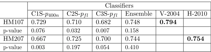
C1S-p400n C2S-pf l C3S-pf l Ensemble V-2004 H-2010

HM107 0.729 0.710 0.682 0.748 0.794

p-value 0.076 0.032 0.007 0.158

HM207 0.667 0.725 0.700 0.744 0.754

p-value 0.003 0.197 0.054 0.410

Table 3: Haydn and Mozart String Quartet classification accuracies in leave-one-out cross-validation. The ta-ble presents the classification accuracies of each individual classifier C1S-p400n, C2S-pf land C3S-pf land their

ensemble. It also shows the accuracies reported by van Kranenburg and Backer (2004) (V-2004), and Hille-waere et al. (2010) (H-2010). The highest accuracies per dataset are highlighted in bold type. Additionally, the table presents one-tailed binomial test p-values related to the differences between the proposed models and V-2004 and H-2010 on the respective datasets. We tested the hypotheses that the accuracies obtained by the methods proposed by van Kranenburg and Backer (2004) and Hillewaere et al. (2010) are higher that those obtained by each classifier. In both datasets, those accuracies are not significantly higher than the accuracies obtained by the proposed ensemble of classifiers.

less information was used (Wilcoxon signed rank = 89.5, z = 0.616, p = 0.538, n = 20), see blocks (I) and (II) for classifiers C2S and C3S in Table 2. The test statistic is computed as the sum of the positive ranks (Gibbons & Chakraborti, 2011). Then, we evaluated the performance of ensembles on symbolic representations and audio. On the results of both datasets HM107 and HM207, we found no significant difference in the performance of the ensembles when classifying music represented symbolically or as audio files synthesized with horn sound (Wilcoxon signed rank = 19.5, p = 0.875, n = 10), see blocks (II) and (III) in Table 2. There was also no significant difference between the accuracies obtained with symbolic representations and synthetic renderings of string sound (Wilcoxon signed rank = 30.5, p = 0.086, n = 10), see blocks (II) and (IV) in Table 2

19

C1S-p400n C2S-pf l C3S-pf l

HM107 0.378 0.230 0.087 HM207 0.007 0.296 0.097

Table 4: One-tailed, binomial testp-values testing the hypotheses that the accuracies (see Table 3) obtained by the ensemble in leave-one-out cross-validation are higher that those obtained by each individual classifier on both datasets (HM107 & HM207) of the Haydn and Mozart string quartets.

We tested the differences in accuracies achieved by our proposed classifiers and the previous approaches of van Kranenburg and Backer (2004), and Hillewaere et al. (2010) for statistical signifi-cance with a one-tailed binomial test. From thep-values in Table 3, we observe that the classification accuracies of van Kranenburg and Backer (2004) and Hillewaere et al. (2010) are not significantly better than the accuracy of our proposed ensemble of classifiers, which can therefore be claimed to have reached state-of-the-art performance on both datasets. Note that Hillewaere et al. (2010) only evaluated their method on the HM207 dataset, which is an extended version of the HM107 dataset. Finally, we tested the differences between our ensemble of classifiers and each of the individual classifiers in the ensemble using a one-sided binomial test. Thep-values are shown in Table 4. They show that the ensemble is only in some cases significantly better than the individual classifiers (i.e.,

p <0.05).

3.2 Experiment 2: Classifying preludes and fugues by J.S. Bach

3.2.1 Dataset

The Well-Tempered Clavier by J. S. Bach consists of two books (published in 1722 and 1742), each containing 24 preludes and fugues, one in each of the 12 major and 12 minor keys. According to Stein’s (1979) analysis, preludes elaborate around a short motivic subject through harmonic exploration, but are heterogeneous in form. Some preludes are imitative and sectional in Invention

subject stated in one or more voices, alternating with episodes in which motivic material derived from the subject and countersubject is developed.

For this experiment we used three datasets, which we called JSB, JSB-H and JSB-B:

• JSB This dataset consists of MIDI encodings of all 48 preludes and 48 fugues from Bach’s

Well-Tempered Clavier, Books I and II, provided in the MuseData collection.5 For experiments on audio, JSB was rendered to WAV format, synthesized with horn sound as described in section 2.1.2.

• JSB-H This dataset consists of 48 preludes and 48 fugues from Bach’s The Well-Tempered

Clavier in MP3 format (Bach, 1742a), performed by pianist Angela Hewitt.

• JSB-B This dataset consists of 48 preludes and 48 fugues from Bach’s The Well-Tempered

Clavier in MP3 format (Bach, 1742b), performed by harpsichordist Pieter-Jan Belder. .

In a fugue, the voices enter one after the other over the course of the exposition, which imparts a highly distinctive textural character to the beginnings of these pieces. We assumed that this feature (the initial texture) could be used to reliably distinguish a fugue from a prelude. In order to avoid reporting less generalizable results, and to avoid the problem of the “horse” system (Sturm, 2014a), we tested the effect of including and removing the initial section of all images.

3.2.2 Classification results

Table 5 presents the accuracies when the initial section is included, and Table 6 presents the ac-curacies when the initial section is excluded. For piano rolls, we removed the initial 60 pixels. For spectrograms of synthetic audio files, we removed the initial 20 pixels. It can be observed that the classification accuracies when including the initial notes are higher than those when removing the initial notes, compare Table 5 and Table 6. The difference in classification accuracy when including and excluding the initial notes is larger for C1, which extracts features at the large scale, than for C2 and C3.

For the piano and harpsichord audio recordings of theThe Well-Tempered Clavier, we removed the first 10 seconds of all audio recordings such that the spectrograms were generated from signals

21

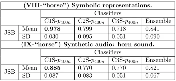
(VIII-“horse”) Symbolic representations.

Classifiers

C1S-p400n C2S-p400n C3S-p400n Ensemble

JSB Mean 0.978 0.799 0.718 0.841

SD 0.030 0.095 0.051 0.090

(IX-“horse”) Synthetic audio: horn sound.

Classifiers

C1S-p400n C2S-p400n C3S-p400n Ensemble

JSB Mean 0.885 0.770 0.770 0.821

SD 0.087 0.083 0.051 0.067

Table 5: Classification accuracies for discrimination between preludes and fugues from The Well-Tempered Clavier by J. S. Bach using symbolic and synthetic audio files, initial notes included. Each classifier’s mean and standard deviation (SD) are reported over the five folds of the cross-validation.

of 30 seconds, starting at second 10, i.e., not including the first 10 seconds, see Table 6, blocks X and XI. In Table 6, we observe that the single C1 classifier performs sometimes better than the ensemble. It could be possible that the texture of preludes and fugues at the large scale is more relevant for discrimination than the texture at the small scale. It is also possible that a more sophisticated ensemble method could achieve better results here.

We found no significant difference in the performance of the ensembles when classifying music represented symbolically or as synthetic audio files (Wilcoxon signed rank = 1, p = 1,n = 5), see blocks VIII and IX. When comparing the performance of the ensemble on symbolic representations and piano recordings, we found no significant difference (Wilcoxon signed rank = 15, p = 0.063,

n= 5), see blocks VIII and X. Finally, we found no significant difference between the performance of the ensemble on symbolic representations and harpsichord recordings (Wilcoxon signed rank = 8.5,

p= 0.375, n= 5), see blocks VIII and XI.

3.3 Experiment 3: Multi-class composer classification

3.3.1 Dataset

In this experiment, we study the ability of the method on multi-class classification, using the following dataset:

• BHTHM. This dataset, introduced by van Kranenburg and Backer (2004), consists of works

by Bach, Handel, Telemann, Haydn and Mozart. The files are encoded as **kern files:6

(VIII) Symbolic representations.

Classifiers

C1S-p400n C2S-p400n C3S-p400n Ensemble

JSB Mean 0.770 0.687 0.729 0.740

SD 0.051 0.072 0.019 0.035

(IX) Synthetic audio: horn sound.

Classifiers

C1S-p400n C2S-p400n C3S-p400n Ensemble

JSB Mean 0.729 0.749 0.709 0.760 SD 0.120 0.062 0.053 0.047

(X) Audio recordings by pianist Angela Hewitt.

Classifiers

C1A-sp30s C2A-sp30s C3A-sp30s Ensemble

JSB-H Mean 0.700 0.616 0.554 0.618 SD 0.090 0.044 0.062 0.092

(XI) Audio recordings by harpsichordist Pieter-Jan Belder.

Classifiers

C1A-sp30s C2A-sp30s C3A-sp30s Ensemble

JSB-B Mean 0.718 0.616 0.616 0.658 SD 0.089 0.095 0.104 0.132

23

– J. S. Bach: 40 cantata movements, 33 fugues from the Well-Tempered Clavier, 11 move-ments from The Art of Fugue, 8 movements from the violin concertos, and 9 fugues for organ.

– G. F. Handel: 39 movements from the Concerti Grossi op 6, and 14 movements from the trio sonatas op. 2 and op. 5.

– G. Ph. Telemann: 30 movements from the church cantates, and 24 movements from the

Musique de table

– F. J. Haydn: 54 movements from the string quartets.

– W. A. Mozart: 53 movements from the string quartets.

Audio files were rendered to WAV format, synthesized with horn sound as described in sec-tion 2.1.2. This dataset is a superset of the Haydn and Mozart string quartet movementsHM107. The dataset BHTHMcontains 9 fugues for organ by Bach instead of 14 as described by van Kra-nenburg and Backer (2004). When reconstructing the dataset, we excluded the pieces marked as being possibly by Wilhelm Friedemann Bach.

3.3.2 Classification results

The classification results of the multi-class recognition task are presented in Table 7. As in previous experiments, the recognition rates between symbolic and audio representation are similar. However, there is a notable difference between the classification accuracies obtained in Experiment 1, on discriminating Haydn from Mozart, and the accuracies obtained on discriminating Bach, Handel, Telemann, Haydn and Mozart, see Table 2, blocks (II) and (III) and Table 7, blocks (V) and (VI). It seems possible that the drop in classification accuracy reported in this experiment on discriminating between five composers is due to the greater number of classes and a class imbalance, as about half of the number of samples is of the class Bach.

(V) Symbolic representations (excerpts).

Classifiers

C1S-p400n C2S-p400n C3S-p400n Ensemble

BHTHM. Mean 0.584 0.607 0.492 0.565 SD 0.028 0.050 0.021 0.033

(VI) Synthetic audio (excerpts).

Classifiers

C1S-sp400n C2S-sp400n C3S-sp400n Ensemble

BHTHM. Mean 0.615 0.623 0.601 0.623 SD 0.052 0.048 0.071 0.054

Table 7: Classification accuracies on multi-class composer recognition for dataset introduced by van Kranen-burg and Backer (2004) using symbolic representations of music and synthetic audio files. Each classifier’s mean and standard deviation (SD) are reported over the five folds of the cross-validation.

the results of our method and those of van Kranenburg and Backer (2004) and Hontanilla et al. (2013), as there is an evident difference in the classification accuracies, and the datasets used on each study are slightly different, as mentioned in section 3.3.1.

4

Discussion

In this study, our aim was to design a general method for music classification applicable to symbolic representations and audio recordings. We have shown that the performance of individual classifiers based on excerpts of music is comparable to the performance of individual classifiers using small time-scale segments. However, the ensemble was not more accurate than individual classifiers. Possibly, we would need to exchange one of the k-NN based classifiers with another algorithm or use a more sophisticated ensemble method.

Our approach was evaluated on datasets where discriminative features do not rely on timbre information. For our method to be competitive on datasets where timbre is a relevant style descrip-tor, we might need to incorporate strategies to extract timbre features. On the other hand, since the proposed method is image-based, and does not use timbral information for its predictions, it can potentially be extended to deal with graphical notation systems, e.g., scores, tablature, neumatic notation, etc.

25

a deep convolutional neural network. This is also appealing, as it may lead to musical insight by inspecting the learnt filters.

5

Conclusions

We have introduced a general convolution-based method on pitch–time representations for classifica-tion of symbolic and audio representaclassifica-tions of music. Our evaluaclassifica-tions were carried out using datasets of baroque and classical music, where timbre might not play a relevant role in style discrimination. Our ensemble classifier performs at a level comparable to state-of-the-art methods (Hillewaere et al., 2010; van Kranenburg & Backer, 2004), when evaluated on two datasets of the Haydn and Mozart string quartets. We have shown that the performance of individual classifiers based on excerpts of music is comparable to the performance of individual classifiers using small time-scale segments, and that their outputs can be complementary for ensembling. However, in multi-class composer recognition, methods specialized for classifying symbolic representations of music (Hontanilla et al., 2013; van Kranenburg & Backer, 2004) are more accurate than our proposed method. Additionally, we evaluated our proposed classifiers on symbolic representations, synthetic audio and two different recordings of The Well-Tempered Clavier by J.S Bach, demonstrating the versatility and effec-tiveness of our method. We found no significant difference between the accuracies obtained using symbolic representations, synthetic audio and recorded audio. Our experiments were conducted on baroque and classical music, but we expect our classifiers to generalize to other styles of music and periods of time, where timbre is not an important style discriminator. The proposed method could potentially be extended to deal with music represented in a variety of graphical notation systems such as scores, tablature, neumatic notation, etc.

preliminary experiments with small (two-layered) CNNs. Preliminary investigation of the filters learned by these networks suggests that these filters may correspond to distinctive pitch and rhyth-mic patterns. Nevertheless, more systematic experiments with these networks are required before drawing stronger conclusions. An interesting approach would be to use techniques such as differ-ential saliency maps (Schl¨uter, 2016), which help to visualize which inputs of a neural network lead to a particular prediction, to analyze musical characteristics of pieces in the same style or by the same composer (or to determine which characteristics of a piece lead to its misclassification). In our future work, we also intend to explore more complex deep learning architectures for style recognition.

6

Acknowledgments

The work for this paper carried out by G. Velarde, D. Meredith, C. Cancino Chac´on and M. Grachten was done as part of the EC-funded collaborative project, “Learning to Create” (Lrn2Cre8). The project Lrn2Cre8 acknowledges the financial support of the Future and Emerging Technologies (FET) programme within the Seventh Framework Programme for Research of the European Com-mission, under FET grant number 610859. G. Velarde is also supported by a PhD fellowship from the Department of Architecture, Design and Media Technology, Aalborg University. C. Can-cino Chac´on and M. Grachten have also been funded by the European Research Council (ERC) under the EU?s Horizon 2020 Framework Programme (ERC Grant Agreement number 670035, project CON ESPRESSIONE). The authors would like to thank Peter van Kranenburg and Ruben Hillewaere for sharing with us the Haydn and Mozart string quartet datasets; and the anonymous reviewers for their insightful comments.

References

Allwein, E. L., Schapire, R. E., & Singer, Y. (2000). Reducing multiclass to binary: A unifying approach for

margin classifiers. Journal of Machine Learning Research,1(Dec), 113–141.

Arthur, D., & Vassilvitskii, S. (2007). K-means++: The advantages of careful seeding. Proceedings of the

27

Bach, J. S. (1742a). The Well-Tempered Clavier, BWV 846-893. (Recorded by Angela Hewitt. Bach: The

Well-Tempered Clavier [Audio CD]. HYPERION (2009))

Bach, J. S. (1742b). The Well-Tempered Clavier, BWV 846-893. (Recorded by Pieter-Jan Belder. Bach:

The Well-Tempered Clavier [Audio CD]. Brilliant Classics (2009))

Bengio, Y., Courville, A., & Vincent, P. (2013). Representation learning: A review and new perspectives.

IEEE Transactions on Pattern Analysis and Machine Intelligence, 35(8), 1798-1828. doi: 10.1109/

TPAMI.2013.50

Cataltepe, Z., Yaslan, Y., & Sonmez, A. (2007). Music genre classification using MIDI and audio features.

EURASIP Journal on Advances in Signal Processing,2007(1), 1–8.

Choi, K., Fazekas, G., Sandler, M. B., & Cho, K. (2017). Transfer learning for music classification

and regression tasks. In Proceedings of the 18th international society for music information

re-trieval conference, ISMIR 2017, suzhou, china, october 23-27, 2017 (pp. 141–149). Retrieved from

https://ismir2017.smcnus.org/wp-content/uploads/2017/10/12 Paper.pdf

Costa, Y. M., Oliveira, L., Koerich, A. L., Gouyon, F., & Martins, J. (2012). Music genre classification using

LBP textural features. Signal Processing,92(11), 2723–2737.

Daubechies, I., & Maes, S. (1996). A nonlinear squeezing of the continuous wavelet transform based on

auditory nerve models. In A. Aldroubi & M. Unser (Eds.), Wavelets in medicine and biology (pp.

527–546). Boca Raton, FL: CRS Press.

Davies, D. L., & Bouldin, D. W. (1979, April). A cluster separation measure.IEEE Transactions on Pattern

Analysis and Machine Intelligence,PAMI-1(2), 224-227. doi: 10.1109/TPAMI.1979.4766909

de Boor, C. (1978). A practical guide to splines. Now York: Springer-Verlag.

Eerola, T., & Toiviainen, P. (2003). MIDI toolbox: Matlab tools for music research. Jyv¨askyl¨a,

Fin-land: University of Jyv¨askyl¨a. (http://www.jyu.fi/hum/laitokset/musiikki/en/research/coe/

materials/miditoolbox/)

Eisen, C., Baldassarre, A., & Griffiths, P. (n.d.). String quartet. http://www.oxfordmusiconline.com

.zorac.aub.aau.dk/subscriber/article/grove/music/40899. Oxford University Press. (Accessed

9-Oct-2015)

Foleiss, J. H., & Tavares, T. (2016). A spectral bandwise feature-based system for the mirex 2016 train/test

task. Submission to Audio Classification (Train/Test) Tasks of MIREX,2016.

Gibbons, J. D., & Chakraborti, S. (2011). Nonparametric statistical inference. InInternational encyclopedia

of statistical science (pp. 977–979). Springer.

Herlands, W., Der, R., Greenberg, Y., & Levin, S. (2014). A machine learning approach to musically

meaningful homogeneous style classification. In Proceedings of the Twenty-Eighth AAAI Conference

from http://www.aaai.org/ocs/index.php/AAAI/AAAI14/paper/view/8314

Hillewaere, R., Manderick, B., & Conklin, D. (2010). String quartet classification with monophonic models.

In J. S. Downie & R. C. Veltkamp (Eds.), Proceedings of the 11th International Society for Music

Information Retrieval Conference, ISMIR 2010, Utrecht, Netherlands, August 9-13, 2010 (pp. 537–

542). International Society for Music Information Retrieval. Retrieved fromhttp://ismir2010.ismir

.net/proceedings/ismir2010-91.pdf

Hontanilla, M., P´erez-Sancho, C., & I˜nesta, J. M. (2013). Modeling musical style with language models

for composer recognition. In J. M. Sanches, L. Mic´o, & J. S. Cardoso (Eds.), Pattern Recognition

and Image Analysis: 6th Iberian Conference, IbPRIA 2013, Funchal, Madeira, Portugal, June 5-7,

2013. Proceedings (pp. 740–748). Berlin, Heidelberg: Springer Berlin Heidelberg. Retrieved from

http://dx.doi.org/10.1007/978-3-642-38628-2 88 doi: 10.1007/978-3-642-38628-2 88

Karmakar, A., Kumar, A., & Patney, R. (2011). Synthesis of an optimal wavelet based on auditory perception

criterion. EURASIP Journal on Advances in Signal Processing,2011(1), 1–13.

Kay, K. N., Naselaris, T., Prenger, R. J., & Gallant, J. L. (2008). Identifying natural images from human

brain activity. Nature, 452(7185), 352–355.

Keys, R. (1981). Cubic convolution interpolation for digital image processing. IEEE Transactions on

Acoustics, Speech, and Signal Processing,29(6), 1153-1160. doi: 10.1109/TASSP.1981.1163711

Kuncheva, L. I. (2004). Combining pattern classifiers: methods and algorithms. John Wiley & Sons.

LeCun, Y., Kavukcuoglu, K., & Farabet, C. (2010, May). Convolutional networks and applications in vision.

In Proceedings of 2010 IEEE International Symposium on Circuits and Systems (pp. 253–256). doi:

10.1109/ISCAS.2010.5537907

Lidy, T., Rauber, A., Pertusa, A., & I˜nesta, J. M. (2007). Improving genre classification by combination of

audio and symbolic descriptors using a transcription systems. In S. Dixon, D. Bainbridge, & R. Typke

(Eds.),Proceedings of the 8th International Conference on Music Information Retrieval, ISMIR 2007,

Vienna, Austria, September 23-27, 2007 (pp. 61–66). Austrian Computer Society. Retrieved from

http://ismir2007.ismir.net/proceedings/ISMIR2007 p061 lidy.pdf

Lidy, T., & Schindler, A. (2016). Parallel convolutional neural networks for music genre and mood

classifi-cation. MIREX2016.

Mandel, M. I., Devaney, J., Turnbull, D., & Tzanetakis, G. (Eds.). (2016). Proceedings of the 17th

inter-national society for music information retrieval conference, ISMIR 2016, new york city, united states,

august 7-11, 2016.

Meredith, D. (2006). The ps13 pitch spelling algorithm. Journal of New Music Research, 35(2), 121–159.

Retrieved fromhttp://dx.doi.org/10.1080/09298210600834961 doi: 10.1080/09298210600834961

29

Perspectives on Learning and Memory (pp. 105–119). Hillsdale, NJ: Erlbaum.

Ogihara, M., & Li, T. (2008). N-gram chord profiles for composer style representation. InProceedings of the

9th international conference on music information retrieval (ismir 2008)(pp. 671–676). Philadelphia,

PA..

Oramas, S., Nieto, O., Barbieri, F., & Serra, X. (2017). Multi-label music genre classification from audio, text

and images using deep features. InProceedings of the 18th international society for music information

retrieval conference, ISMIR 2017, suzhou, china, october 23-27, 2017 (pp. 23–30). Retrieved from

https://ismir2017.smcnus.org/wp-content/uploads/2017/10/126 Paper.pdf

Paul, E. S., & Kaufman, S. B. (2014). The philosophy of creativity: New essays. Oxford University Press.

Pons, J., Lidy, T., & Serra, X. (2016). Experimenting with musically motivated convolutional neural

networks. InProceedings of the 14th International Workshop on Content-Based Multimedia Indexing

(CBMI 2016). Bucharest, Romania.

Pribram, K. H. (1986). Convolution and matrix systems as content addressible distributed brain processes

in perception and memory. Journal of Neurolinguistics, 2(1), 349–364.

Rush, J. C., & Sabers, D. L. (1981). The perception of artistic style.Studies in Art Education,23(1), 24–32.

Sapp, C., & Liu, Y.-W. (2015). The Haydn/Mozart String Quartet Quiz. (http://qq.themefinder.org

(Accessed 26-Dec-2015))

Schl¨uter, J. (2016). Learning to pinpoint singing voice from weakly labeled examples. In M. I. Mandel,

J. Devaney, D. Turnbull, & G. Tzanetakis (Eds.), Proceedings of the 17th international society for

music information retrieval conference, ISMIR 2016, new york city, united states, august 7-11, 2016

(pp. 44–50). Retrieved from https://wp.nyu.edu/ismir2016/wp-content/uploads/sites/2294/

2016/07/315 Paper.pdf

Sch¨orkhuber, C., Klapuri, A., Holighaus, N., & D¨orfler, M. (2014). A Matlab toolbox for efficient perfect

reconstruction time-frequency transforms with log-frequency resolution. InAudio Engineering Society

Conference: 53rd International Conference: Semantic Audio. London, UK.

Snowden, R. J., Thompson, P., & Troscianko, T. (2012). Basic vision: An introduction to visual perception.

Oxford: Oxford University Press.

Stein, L. (1979). Structure & style: the study and analysis of musical forms. Summy-Birchard Music.

Sturm, B. L. (2014a). A simple method to determine if a music information retrieval system is a “horse”.

IEEE Transactions on Multimedia,16(6), 1636–1644.

Sturm, B. L. (2014b). A survey of evaluation in music genre recognition. InAdaptive multimedia retrieval:

Semantics, context, and adaptation (pp. 29–66). Springer.

Tuia, D., Volpi, M., Mura, M. D., Rakotomamonjy, A., & Flamary, R. (2014). Automatic feature learning for

Sensing,52(10), 6062-6074. doi: 10.1109/TGRS.2013.2294724

Tzanetakis, G., Ermolinskyi, A., & Cook, P. (2003). Pitch histograms in audio and symbolic music

informa-tion retrieval. Journal of New Music Research,32(2), 143–152.

van Kranenburg, P., & Backer, E. (2004). Musical style recognition—a quantitative approach. In R. Parncutt,

A. Kessler, & F. Zimmer (Eds.),Proceedings of the Conference on Interdisciplinary Musicology (CIM04)

Graz, Austria, April 15-18, 2004 (pp. 106–107).

van Kranenburg, P., Volk, A., & Wiering, F. (2013). A comparison between global and local features

for computational classification of folk song melodies. Journal of New Music Research, 42(1), 1-18.

Retrieved from http://dx.doi.org/10.1080/09298215.2012.718790 doi: 10.1080/09298215.2012

.718790

Velarde, G., Weyde, T., Cancino Chac´on, C. E., Meredith, D., & Grachten, M. (2016). Composer recognition

based on 2d-filtered piano-rolls. In M. I. Mandel, J. Devaney, D. Turnbull, & G. Tzanetakis (Eds.),

Proceedings of the 17th International Society for Music Information Retrieval Conference, ISMIR 2016,

New York City, United States, August 7-11, 2016(pp. 115–121). Retrieved fromhttps://wp.nyu.edu/

ismir2016/wp-content/uploads/sites/2294/2016/07/063 Paper.pdf

Velarde, G., Weyde, T., & Meredith, D. (2013). An approach to melodic segmentation and classification

based on filtering with the haar-wavelet. Journal of New Music Research,42(4), 325–345. Retrieved

from http://dx.doi.org/10.1080/09298215.2013.841713 doi: 10.1080/09298215.2013.841713

Wu, M.-J., Chen, Z.-S., Jang, J.-S. R., Ren, J.-M., Li, Y.-H., & Lu, C.-H. (2011). Combining visual and

acoustic features for music genre classification. InMachine Learning and Applications and Workshops