New methods for automatic quantification of microstructural features using digital image processing

New methods for automatic quanti

fi

cation of microstructural features

using digital image processing

Andrew Campbell

⁎

, Paul Murray

, Evgenia Yakushina

, Stephen Marshall

, William Ion

a

Advanced Forming Research Centre (AFRC), Dept. of Design Manufacture and Engineering Management, University of Strathclyde, Glasgow, United Kingdom b_{Department of Eletronic and Electrical Engineering, University of Strathclyde, Glasgow, United Kingdom}

H I G H L I G H T S

•A fully automated procedure for micro-structural analysis is proposed. •Measurement accuracy is validated on

Ti6Al4V microstructures.

•Grain size measurements are consistent with results from existing procedures. •Much faster measurement times when

compared with manual procedures.

G R A P H I C A L A B S T R A C T

a b s t r a c t

a r t i c l e i n f o

Article history:

Received 27 October 2017

Received in revised form 14 December 2017 Accepted 26 December 2017

Available online 27 December 2017

Thermal and mechanical processes alter the microstructure of materials, which determines their mechanical properties. This makes reliable microstructural analysis important to the design and manufacture of components. However, the analysis of complex microstructures, such as Ti6Al4V, is difficult and typically requires expert ma-terials scientists to manually identify and measure microstructural features. This process is often slow, labour in-tensive and suffers from poor repeatability. This paper overcomes these challenges by proposing a new set of automated techniques for 2D microstructural analysis. Digital image processing algorithms are developed to iso-late individual microstructural features, such as grains and alpha lath colonies. A segmentation of the image is produced, where regions represent grains and colonies, from which morphological features such as; grain size, volume fraction of globular alpha grains and alpha colony size can be measured. The proposed measurement techniques are shown to obtain similar results to existing manual methods while drastically improving speed and repeatability. The benefits of the proposed approach when measuring complex microstructures are demon-strated by comparing it with existing analysis software. Using a few parameter changes, the proposed techniques are effective on a variety of microstructure types and both SEM and optical microscopy images.

© 2018 The Authors. Published by Elsevier Ltd. This is an open access article under the CC BY license (http:// creativecommons.org/licenses/by/4.0/). Keywords:

Microstructure analysis Segmentation Watershed algorithm Titanium alloy

1. Introduction

The microstructure of a metal often reveals important information about its mechanical properties, such as strength, ductility, yield stress, tensile strength, hardness and surface roughness among others[1,2]. In fact, the ability to control the microstructure of a manufactured part has ⁎ Corresponding author.

E-mail address:[email protected](A. Campbell).

https://doi.org/10.1016/j.matdes.2017.12.049

0264-1275/© 2018 The Authors. Published by Elsevier Ltd. This is an open access article under the CC BY license (http://creativecommons.org/licenses/by/4.0/).

Contents lists available atScienceDirect

Materials and Design

now become a key aspect of many manufacturing techniques[1]. Differ-ences in thermal and mechanical processing can produce different mi-crostructures and therefore components with different properties. Carefully controlling these factors allow material properties to be re-fined to best suit a specific application [3]. Development of new manufacturing processes or models, and the existing design and manufacturing of high value components, must consider the effect of the microstructure of the material. This makes microstructural analysis essential for many academic and industrial projects.

Microstructures can contain a variety of different features, each often requiring different analysis procedures to measure them. Several techniques have already been proposed to measure a range of micro-structural features, however, all have limitations that still need to be addressed.

The American Society for Testing and Materials (ASTM) produce in-dustrially recognised standards for the analysis of material microstruc-ture. The ASTM E112 standard describes streamlined methods for manually measuring average grain size based on linear intercepts of line segments[4]. A set of lines are overlaid on an image and marked at locations where they cross a boundary between grains. The mean dis-placement between these marks gives an approximation of the mean grain size of that microstructure. Typically, only a subset of grains is measured, with 300 measurements required for statistically valid re-sults. If the set of lines is placed randomly, then the result would be free from bias but the aspect ratio of grains could not be calculated. Manually selecting lines, so that they run the length and width of each grain, allows for more detailed measurement but at the cost of exposing the result to bias, as users can select which grains to measure. The ASTM E562 standard describes techniques to measure volume fraction based on point counting[5]. A set of points are distributed throughout an image and an expert then specifies which points lie within each phase. The percentage of points marked within a single phase gives the volume fraction of that phase.

Implementing these standards is very labour intensive, making them slow and inefficient. The E562 standard estimates a measurement time of 15 mins per image for an experienced user[5], and our experi-ments show similar times for the E112 standard. As defining the loca-tion of grain boundaries is often subjective, such methods are also prone to human error and poor repeatability. The latter is of particular concern in the E112 standard which estimates inter-operator repeat-ability at ±16% for measurements in micrometres[4]. This variability makes small microstructural changes difficult to detect and may misdi-rect research into new manufacturing processes or microstructural refinement.

The procedures described above are based on 2D imaging technolo-gies common in both industry and academia, however, there also exist methods to analyse materials in 3D. 3D techniques based on X-ray to-mography have been applied for the analysis of porosity in metal alloys

[6]and to measure grain orientation and position over time[7]. Similar techniques have been proposed using focus ion beam (FIB) or serial block face scanning electron microscopy (SBFSEM) to produce 3D scans of microstructure, using serial sectioning techniques[8]. As micro-structures are 3D micro-structures these techniques are potentially more accu-rate than 2D scans. However, many of these methods are not as readily available as traditional 2D microscopy. Furthermore, recent research shows that automated analysis of 3D microstructures can be achieved using techniques originally developed in the 2D domain[9]. We there-fore focus on automating procedures based on more ubiquitous 2D im-aging technologies as this is impactful now and is potentially still useful in the future, with opportunities to extend them to 3D.

Digital image processing techniques have been successfully applied to improve 2D analysis procedures in otherfields such as biology[10]

and geology[9,11]as well as to analyse the microstructure of non-me-tallic elements[12]. In recent years image processing techniques have also been proposed to improve microstructural analysis of metals by au-tomating some, or all, of the measurement process[13–17]. Collins et al.

and Tiley et al.[13,14]propose several stereology procedures that can be implemented in the Photoshop extension Fovea Pro. Tiley's work fo-cuses on beta processed lamellar microstructures and Collins extends this to measure bi-modal microstructures. The width of alpha laths is measured by applying a grid of lines at successive 10 degree increments. The length of any segment of these lines that can_fit within a lath is mea-sured and these lengths are used to approximate the average thickness of alpha laths. The volume fraction of alpha phase is found by using thresholding to separate the alpha from the beta phase and computing the percentage of light and dark pixels. Manual input remains necessary for measuring grain and colony size. Yang and Liu[15] also use thresholding for the separation of grain phases. Gaussianfiltering tech-niques are used to reduce the impact of image noise and the pixel values are used to estimate the depth below the machined surface. Zhe et al.

[16]present a method for separating touching globular and lamellar phase. The algorithm searches for concave regions in the alpha phase and splits objects where this concavity is significant. However, this ap-proach cannot split individual grains of the same type. Sosa et al.[17]

developed an automated software tool to measure a variety of micro-structural features such as grain size and volume fraction. Grain size is measured from a segmented image where each segment is assumed to be a grain. To compute this segmentation, adaptive thresholding is used to locate dark or light lines in the image, which are considered to represent grain boundaries. Automated algorithms then complete any gaps in the boundary to form a complete segmentation and the software then measures each region. Phase separation is performed in a similar way as other methods reviewed here. Additionally, the software can also compute the orientation of the image which can help identify lath colonies in microstructural images, although no fully automated method for computing their size is provided.

Some features, such as the volume fraction of alpha phase and width of alpha laths, can be measured relatively successfully by existing tech-niques, as a result these are not investigated further in this study. In-stead we focus on features for which the results of existing automated measurements are less reliable. Of the aforementioned techniques, only Sosa et al.[17]present automated methods for the analysis of alpha grains with all others still requiring manual input to measure this feature. However, the method proposed in[17]relies on boundaries presenting with a dark or light line at their boundary, which is not al-ways possible when imaging many microstructures. This affects the re-liability of measurements of alpha grain size and volume fraction of globular alpha. Measuring the size of alpha lath colonies also remains a manual task in these procedures. We found that, within both industry and academia, manual procedures are currently relied upon to measure the complex microstructures used in our study due to the lack of reliable techniques for identifying and measuring alpha grains.

It is clear that new data processing techniques are needed in order to reduce the time taken to perform microstructural analysis, reduce human error and give repeatable results. Digital image processing theo-retically offers a solution to all these problems. However, existing tech-niques fail to accurately identify many relevant microstructural features. This paper develops new techniques specifically designed to recognise these features. We apply our techniques to measure primary alpha grain size, the volume fraction of globular primary alpha and the size of alpha lath colonies.

2. Material and microstructure

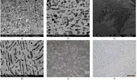
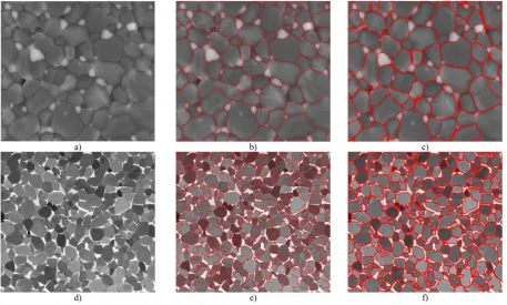
A material's microstructure depends on the type of material and manufacturing processes. A variety of different features may be visible, as indicated by the microstructures shown inFig. 1. For our study, we focus on the titanium alloy Ti6Al4V. The popularity of this alloy[1], par-ticularly within high value manufacturing sectors such as aerospace

techniques developed for this material will be applicable to the micro-structure of other materials.

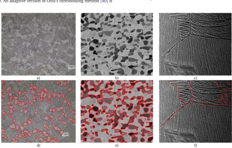
The microstructures were studied using the Quanta FEG 250 Scan-ning Electron Microscope (SEM) and the OM Leica DM12000M Optical Microscope. Ti6Al4V has a microstructure that consists of two distinct phases, an alpha and beta phase, which are distinguishable by image in-tensity. Alpha phase is light and beta phase is dark in optical images, shown inFig. 1e) and f), while the reverse is true in SEM images, shown in the remainder ofFig. 1. Alpha phase investigated in the paper consists of individual grains which can be categorised as either globular or lamellar, depending on their morphology. Investigated beta phase was represented either as a beta matrix,Fig. 1b) and d), or as a mixture of beta phase and alpha platelets, as shown inFig. 1c)_–f). These are sometimes referred to as martensite laths, and often exist in parallel groups separated by thin layers of beta phase. These parallel groups are known as colonies. The microstructure of this material can be categorised into three main types; globular, bimodal or fully lamellar

[1]. All of the aforementioned microstructure types are studied in this work to ensure the generalisation of our techniques. Different types of microstructure morphology were obtained after different thermo-me-chanical processes. Examples of the differences between our micro-structures are shown inFig. 1.

Existing research has identified the size of equiaxed alpha grains as a key factor in determining material properties, with yield strength in particular being directly related to mean grain size[19]. For example, the analysis of primary alpha phase is necessary for recent work aimed at creating ultrafine grained materials, where grain size and elon-gation are important[20,21]. Additionally, the volume fraction of glob-ular alpha, size of alpha lath colonies, volume fraction of alpha phase and width of alpha laths are all considered significant[13,14]. This paper focuses on approaches for calculating the mean size of primary alpha grains, the volume fraction of globular alpha and colony size as these morphological features are important and often currently require time consuming manual methods to measure.

3. Digital image analysis

A popular method of measuring image features is to use algorithms that automatically partition an image into a set of regions of interest. This process is commonly called Segmentation[22]. To measure grains in a microstructure, segmentation algorithms can be designed to locate grain boundaries and label all pixels within a single continuous bound-ary as belonging to one grain. From this segmentation a variety of mea-surements can be made using established methods[23]. A key benefit of this approach is in analysis time, with the application of automated image segmentation in otherfields producing measurements in sec-onds, or even milliseconds for small images[24]. Measurement by a predetermined software algorithm also allows results to be repeated without any inter-operator variation.

The key challenge when using automated segmentation algorithms is ensuring the segmentation produced accurately represents the fea-tures to be measured. This is widely considered the most difficult task in this type of image analysis and methods capable of segmenting im-ages for one application often do not work in others[22,25]. Image pro-cessing techniques such as the Watershed Algorithm[26], Active Contour Models[27], Hit-or-Miss transforms[28]and Clustering[29]

have all been applied to segment images in a range of applications, from microscopic cells to large sheets of ice[10,11,30,31]. Each method has its own advantages but none of the aforementioned techniques are able to reliably segment features of Ti6Al4V microstructures without substantial adjustments.

computing markers that estimate locations of alpha grains and colonies in a microstructural image and reduce over-segmentation.

4. Challenges when performing microstructural analysis

Microstructural images have a series of inherent properties that make analysis difficult for both automated and manual techniques. Any approach for measuring the size of grains or colonies relies on the ability to identify the boundaries of these features. Alpha and beta phase present as light and dark regions in an SEM image so the bound-aries between these are often quite clear. However, grains of the same phase are typically more difficult to distinguish. As an SEM gives a high contrast images, adjacent grains often differ in intensity, even when they are of the same phase. Optical microscopes provide lower contrast, so there is often no visible boundary between grains.Fig. 2

shows clusters of equiaxed grains imaged using each technology to il-lustrate this.

As well as visible contrast changes between grains the shape of the grain can also be used to locate boundaries. Grains are approximately el-liptical and do not normally feature any concave regions. Therefore, such concavities often indicate the presence of an overlap between two adjacent grains. These concavities are typically more distinct when circular grains overlap, compared to more elongated grains. Con-cavities are equally visible in both SEM and optical images.

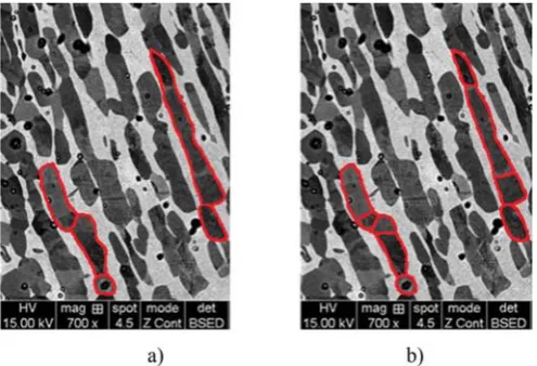
Deciding which contrast variations and concavities are sufficient to indicate a boundary is difficult, even for experienced materials scien-tists. Microscopic images often suffer from noise which can obscure grain boundaries or even create the appearance of boundaries that do not exist. This is particularly common in images produced using an SEM. Grain boundaries are also not perfectly smooth meaning deforma-tion or phase transformadeforma-tion could create concavities in a grain, but not indicate an overlap between adjacent grains. There is no explicit rule for

distinguishing between these noise sources and true boundaries, so manual processes rely on an operator's experience to make the decision. The subsequent measurements are therefore subjective and dif_ficult to repeat. This is demonstrated inFig. 3which shows a microstructure containing elongated alpha grains, with two regions manually seg-mented by different materials scientists. The result is very different with the same area divided into 5 grains by one user and 9 by the other. Further difficulties are produced by etching and polishing, which is usually required prior to microscopic analysis to ensure microstructural features are visible. This is a non-trivial task and can cause scratches or other artefacts to appear on the microstructural image, some of which can be seen inFig. 3. This rarely causes problems in manual analysis but could be more problematic for automated approaches as they need to be taught to distinguish this from useful information.

5. New microstructural analysis method

In this section we present innovative image processing techniques to automate the analysis of different morphological types of Ti6Al4V mi-crostructure. The methodology we use to detect and measure micro-structural features is shown in the block diagram inFig. 4. The same approach is used for both alpha grain and lath colony measurements, however, different modifications are made to the Watershed Algorithm in each case for correct operations. Where appropriate, the influence of different parameters in our algorithms is discussed to demonstrate how these methods can be adapted to suit different applications and datasets.

5.1. Filtering

The initial microstructural image isfirstfiltered to reduce noise while preserving intensity differences between adjacent grains. We found Gaussianfiltering[25]to be effective, in line with previous re-search[15], however thisfilter can also cause distortion. The size of thefilter determines the extent of both noise reduction and distortion, so should be adjusted depending on the application to ensure the best results. SEM images contain more noise than optical ones so require a largerfilter. Images showing thin laths would see these laths hidden by even a small amount of distortion, so smallerfilters are needed. For the Ti6Al4V microstructures in our dataset, the best results were achieved using a 5 × 5filter for SEM images and a 3 × 3filter for optical images or images where laths were present.

5.2. Watershed Transform

Image segmentation is performed using the Watershed Transform

[26]. This technique considers the image as a topographic surface[32]

andfloods this surface from local minima. Whenfloods from different sources meet, they are prevented from merging and these locations are marked as boundaries. The transform returns a uniquely labelled set of regions fully enclosed by these boundaries. If performed correctly on our dataset, each region in the segmented data will represent a single microstructural feature. We use a marker based Watershed Transform

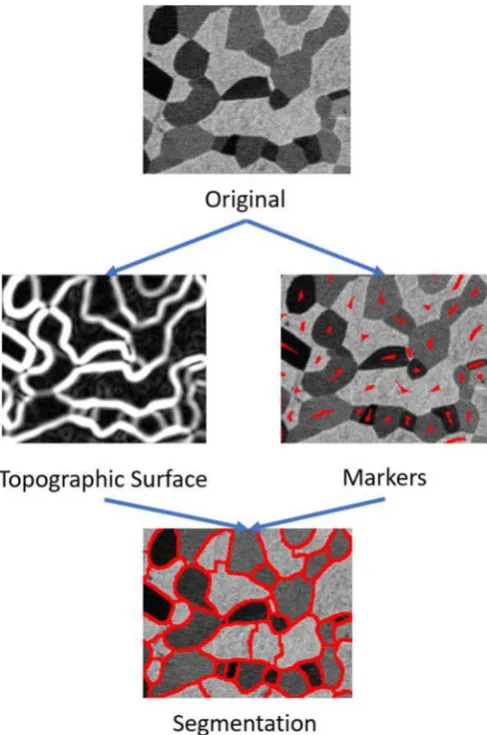
[26], whichfloods the image exclusively from pre-defined locations known as markers, rather than from all local minima. This has been shown to improve segmentation accuracy, particularly in reducing over-segmentation[33–35], making it ideally suited to segmenting mi-crostructural images. The marker based Watershed Transform requires two inputs, the topographic surface, estimating grain boundaries, and the markers, estimating grain locations. The transform uses these esti-mates tofind a complete image segmentation by placing boundaries on ridgelines of the topographic surface that are between adjacent markers. These ridgelines should correspond to the edges of segmented objects, as shown inFig. 5. Using a suitable topographic surface and set of markers are critical to the accuracy of segmentation. Computing ap-propriate markers is a difficult task and often requires bespoke Fig. 2.Difference between SEM and optical imaging technologies in terms of grain

boundary visibility and noise where a) is a cluster of alpha grains in an SEM images and b) is a similar cluster in an optical image.

techniques to be designed that are dependent on the feature being marked. We propose distinct, novel techniques to mark alpha grains and lath colonies. We also propose different methods for computing the topographic surface in each case.

5.2.1. Globular alpha segmentation

To segment alpha grains, we use the gradient magnitude function as the topographic surface[25]. This is an image transform where the value of each pixel in the output image corresponds to the change in intensity at that location in the original image. Using the output of this function as the topographic surface will result in boundaries being placed where the most significant intensity changes exist between markers.

For alpha grains, edge detection[22]is used tofind areas in the image where significant variations in intensity occur. The sensitivity of this edge detection,Es, determines the magnitude of intensity change in the image that suggests the presence of a grain boundary. We then

place a marker in the centre of areas which are at least partially enclosed by these edges. Doing so takes account of both image intensity and ob-ject shape, making our approach effective for optical and SEM images. In a similar way, we also set constraints on the Watershed so thatfloods cannot pass from one phase of material to another. Edge detection, with lower sensitivity, is used to locate only large intensity changes which typically indicate boundaries between alpha and beta phases with the Watershed being forbidden to allow any region to cross this boundary. This helps to ensure that each identified grain exists in only one phase of the material.

5.2.2. Lath colony segmentation

For segmenting colonies we use the gradient orientation of the image as the topographic surface, computed using Sobel Filters[22]. The gradient orientation is the orientation of greatest intensity change for a given image location. This is measured counter clockwise from the positive x-axis. Using the gradient orientation as the topographic surface results in boundaries placed where laths are closest to being perpendicular.

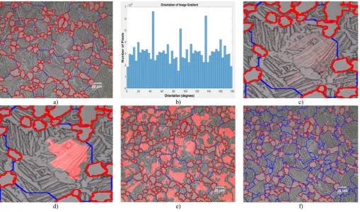
If each lath was marked by the method described for alpha grain analysis, it would be possible to segment them and compute the angle of orientation of individual laths[36]. Laths at similar orientations could then be grouped to mark colonies. However, as laths are often ex-tremely thin and have unclear boundaries compared to equiaxed alpha grains, we are unable to segment and study individual laths. To over-come this challenge, we use the gradient orientation to assess each pixel, rather than computing orientation per lath. Pixels with similar orientation values are then grouped to mark colonies. The laths in Ti6Al4V are separated by thin layers of beta phase. As alpha laths and beta phase have significantly different intensity in microstructural im-ages, the greatest gradient will typically occur perpendicular to the ori-entation of the lath. For fully lamellar microstructures containing only a few colonies this technique can be applied directly. However, in bi-modal microstructures many colonies of laths are typically visible, mak-ing common orientations difficult to identify. To solve this an unmodi-fied Watershed Transform[26]is applied to the inverse of the alpha grain segmentation, to split the laths into smaller regions, as shown in

Fig. 6a). The smaller number of colonies that exist in each region makes the dominant lath directions easier to identify. Due to noise in the image, a wide variety of angles are recorded, however, values representing the orientation of the laths will occur more frequently. A histogram, shown inFig. 6b), can be used to identify the most common angles that occur in the image. Pixels at a peak angle, +/−a constant,Ar, are then isolated, as shown inFig. 6c). Mathematical morphology[25]is used to group pixels that are within a spacing factor,Ls, of each other into a single marker representing the colony, shown inFig. 6d).Aris used to account for both errors in orientation measurement and the fact that laths are not always aligned perfectly within the colony, so is typically set relatively high at around 15°.Lsis the distance between laths at the same angle that are considered to be within the same col-ony. The best value is usually the same as the width of the widest lath in the image.Fig. 6e) shows the complete set of markers for laths in the microstructural image andFig. 6f) shows the resulting segmenta-tion of the image into separate colonies using these markers.

Fig. 4.Flow chart of main steps in algorithm for measuring the size of microstructural features.

5.3. Region merging

We propose a new approach to reduce over-segmentation errors produced by the Watershed Transform by merging adjacent regions whose properties suggest they belong to the same feature. Similar ap-proaches have been applied successfully in other image segmentation methods[37,38].

Our approach uses a region adjacency graph[39]. This is a graph,G = (V,E), where each vertex,V, is a region of the image and edges,E_⊂ Vi×Vj, connect vertices only when the regions share a common bound-ary, as illustrated inFig. 7a) with vertices in blue and edges in green. For each edge, a weight,wij, is typically computed based on the similarity of the regions (vertices) it connects. When the weight of this edge exceeds a predetermined threshold, edges are removed from the graph such that only edges between similar regions remain, as shown inFig. 7b). Any

internal boundaries between regions connected by an edge are then re-moved and the encapsulated region is categorised as a single grain. The updated segmentation is shown inFig. 7c).

Determining suitable edge weights and merging thresholds is criti-cal to the success of the proposed region merging method. The more ac-curately the properties of objects can be predicted in advance the more precisely these can be set and the more effective this technique is. In mi-crostructural analysis, it is often difficult to predict grain properties and, therefore, selection of these weights and thresholds is difficult. To deal with this we define 3 separate weights and thresholds to enable each pair of regions to be examined by 3 separate criteria.

We based edge weights on; the length of boundaries,B, the mean in-tensity of pixels in the region,I, and region size,S. Thefirst weight,w1ij ¼ Bc

minðBi;BjÞ, is the percentage of the boundary of the smaller grain that is Fig. 6.Analysis of optical image where a) segmentation of non-equiaxed alpha regions (blue) based on equiaxed alpha grain segmentation (red), b) histogram of gradient orientation measured counter clockwise from the positive x-axis, c) locations where peak gradient value x is returned, d) markers for a lath of orientation x, e) complete set of markers for the entire image and f) segmentation of alpha lath colonies. (For interpretation of the references to colour in thisfigure legend, the reader is referred to the web version of this article.)

a common boundary,Bc, with the adjacent grain. The second weight, w2ij=Ii−Ij, is the difference in intensity between each grain. The third weight,w3ij= min (Si,Sj), is the size of the smaller of the two re-gions. We use the mean diameter of the regions as the size but other metrics could also be used. Thresholds,TB,TI,TS, are then used to judge each of these weights and the merge test,M, is positive when regions should merge.TBshould be set as the maximum amount of boundary that is expected to be shared between grains,TIset as the maximum in-tensity difference expect between regions of the same grain andTSset as the smallest possible grain size expected in the microstructure. Regions are set to merge either when one region is very small, indicating it is probably caused by an artefact, or when regions share both a large com-mon boundary and a similar intensity.

M¼ 1 ifw1ijNTB; w2ijNTIorw3ijbTS

0 otherwise

ð1Þ

Although it is difficult to refine the optimum parameters to correct general segmentation errors due to variations in grain properties, region merging still offers a powerful method to reduce the impact of scratches and artefacts on the images as their features are typically distinct from regular grains. Thresholds could be set in Eq.(1)that would merge arte-facts, and regions split by a scratch, to an adjacent grain without signif-icantly affecting the rest of the segmentation. In cases where more specific properties of microstructural features are known in advance, a more extensive merging criterion could be used to obtain more accurate results.

5.4. Phase separation

The Watershed Transform produces a complete segmentation of the image, including all phases of material. Before measurements can be taken we must distinguish which regions are alpha phase and which are beta phase. Thresholding the original image provides an estimate of phase separation, as each phase normally is of signi_ficantly different intensity. An adaptive version of Otsu's thresholding method[40]is

used to automatically select a suitable threshold for each region of each image. This prevents inconsistency in illumination from causing phases to be misidenti_fied. The user must indicate to the software whether images are from SEM or optical microscopes, since alpha phase is dark in the former and light in the latter. For measurements of primary alpha grains, a morphological opening[25]is used to remove any coarse alpha platelets, such as shown inFig. 1e), so that these are not categorised as primary alpha.

Due to noise in the images, each grain will contain some pixels marked as alpha and some that are marked as beta. A threshold is set to determine if a grain belongs to a particular phase. If set too high then some grains would be ignored from measurement. We normally set the threshold high for alpha grain measurements as measuring fewer grains is preferable to measuring grains incorrectly.

5.5. Measurement

After phase separation, each grain is represented by a single group of pixels where each pixel is adjacent to at least one other pixel in the group. This configuration is called a connected component (CC) and several techniques have been defined to measure their properties[36]. Wefit an ellipse to this region to measure the length, L, and width, D, for each grain. These values are used to compute the mean grain size, GS, and globular volume fraction,VFG, using Eqs.(2) and (3)wheren is the number of grains measured.

GS_¼X n

1 LnþDn

2 ð2Þ

VFG¼ ∑n

1 1 if Ln DnN

2 0 otherwise 8

< :

n ð3Þ

6. Experimental results

In this section we evaluate the performance of our proposed analysis techniques by comparing the automatically produced measurements with those from existing manual procedures. Average alpha grain size, colony size and volume fraction of globular alpha phase are all consid-ered using globular, bi-modal and fully lamellar microstructures. We also compare our method against an existing analysis technique used in MiPar software[17], to further demonstrate the benefits of our approach.

6.1. Dataset and experimental procedure

A variety of Ti6Al4V samples were produced, each using different thermal and mechanical processes to ensure a varied dataset. For each sample, up to 5 microstructural images were taken using either an SEM or optical microscope. Measurements were taken on a sample by sample basis with metallurgists permitted to select the images from each sample they felt were most suitable to measure. To keep our com-parison consistent the software was set to only measure the same im-ages selected by the metallurgist, rather than all imim-ages in the sample. In total 26 different material samples and around 100 images were used in this study. We elected to measure both equiaxed alpha grains and colony sizes by manually drawing lines across the length and width of each grain rather than using grid based methods as this allowed the aspect ratio of each grain to be measured. Globular volume fraction was computed from the same set of measurements by dividing the number of grains with an aspect ratiob2 by the total number of grains measured. For each sample, a minimum of 300 measurements were taken when assessing mean alpha grain size. For our fully lamellar microstructures, the number of visible colonies wasb300 so all colonies were measured. Of the 26 samples produced 16 were bimodal, 6 were globular and 4 were lamellar. 2 of the 16 bimodal microstructures contained measurable lath colonies. Examples of each microstructure type are shown inFig. 1. For each type of microstructure all relevant properties were assessed.

The automated procedures were implemented in a software package built using the MATLAB programming language. Unlike manual methods the software measured every grain in each image rather than a subset of 300, leading to more grain measurements per image. The software allows an image to be produced, showing where it has de-tected grain boundaries, examples of which are shown inFig. 8. This it-self indicates how likely the result is to be accurate and provides feedback, allowing the user to decide if any parameters need to be ad-justed. For alpha grain analysis, the_first image from each sample was used to set parameter, Es, by adjusting this parameter tofind a suitable looking segmentation. The user did not know any numerical results at this stage and the parameter remained unchanged for all other images in that sample. Parameters were set for lath analysis in the same way with Ls being adjusted for each sample and Arbeing set at 15° through-out. For all samples, the merging parameters Bc= 0.4, Ti= 10 and TG=

1 were chosen by manual visual inspection of a few microstructures. These values reduced the effects of scratches and artefacts but, for gen-erality purposes this was not re_fined to suit any particular microstruc-ture type in our study.

When comparing the results, it is important to remember that man-ual measurements cannot be taken as the absolute truth, due to subjec-tivity, bias and human error. As such errors are difficult to quantify, we use the expected inter-operator variation defined in industrially recognised standards[4,5]as an indicator of accuracy. For volume frac-tion, inter-user repeatability of ±10% is expected[5]while grain size standards expect a variation of ±0.5 G between measurement by differ-ent operators[4], which equates to ±16% in micrometres. As previously described, subjectivity is greater when elongated grains exist so less variation would be expected in more globular microstructures. The dif-ference between measurements is recorded inTables 1–4and colour coded with green indicating a close match, red indicating disagreement beyond what would reasonably be expected and amber indicating a dif-ference in measurement that is on the limit of expected inter-operator variations.Table 5gives summary statistics for each feature measured and microstructure type, to illustrate where our methods are most effective.

6.2. Comparison with manual procedures

6.2.1. Grain size

Overall, there is a good correlation in grain size measurements be-tween existing manual procedures and our automated analysis ap-proach. For fully globular microstructures, grain size measurements were typically within 0.3_μm for 4_–5_μm grains, as shown inTable 1. The greatest difference between measurements was 0.41μm, which is still comfortably within the expected inter-operator variation. This is a very positive result, particularly given that grains are tightly packed in our microstructure, which often makes automatic segmentation more difficult. For bi-modal microstructures most measurements also closely matched the manual results, with grain sizes of around 10μm and dis-agreement between results under 0.5μm in most microstructures,

Table 1

Grain size measurements of fully globular microstructure.

Sample Grain size (µm)

Manual Auto Difference

1 4.72±0.76 4.51 −0.21

2 5.01±0.80 5.04 +0.03

3 4.86±0.78 4.62 −0.24

4 5.42±0.87 5.14 −0.28

5 4.18±0.67 4.59 +0.41

6 4.82±0.77 4.62 −0.2

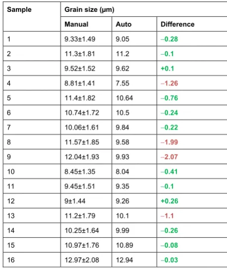
Table 2

Size and Volume Fraction Measurements of Bi-Modal Microstructures.

Sample Grain size (µm)

Manual Auto Difference

1 9.33±1.49 9.05 −0.28

2 11.3±1.81 11.2 −0.1

3 9.52±1.52 9.62 +0.1

4 8.81±1.41 7.55 −1.26

5 11.4±1.82 10.64 −0.76

6 10.74±1.72 10.5 −0.24

7 10.06±1.61 9.84 −0.22

8 11.57±1.85 9.58 −1.99

9 12.04±1.93 9.93 −2.07

10 8.45±1.35 8.04 −0.41

11 9.45±1.51 9.35 −0.1

12 9±1.44 9.26 +0.26

13 11.2±1.79 10.1 −1.1

14 10.25±1.64 9.99 −0.26

15 10.97±1.76 10.89 −0.08

shown inTable 2. However, there are several cases where results did not match as closely as they did for the globular microstructures. One possi-ble reason for this is that many of the bi-modal microstructures in this study contained more elongated primary alpha than was seen in the fully globular microstructures. The boundaries of these grains are less clear so subjectivity is expected to cause wider variations in these cases, as was illustrated inFig. 3. Microstructures in samples 8 and 9 ap-pear to have large numbers of elongated grains and also exhibit the larg-est difference between results. Despite this, no measurement lies significantly outside the expected inter-operator variation.

The time taken to produce these results is drastically reduced com-pared to manual methods. A typical image containing approximately 150 grains, as shown inFig. 8b), was measured by our software in 3.79 s while it took a materials scientist approximately 15 min to accu-rately measure the same image. Similar differences in time were found for all images in our study. In the microstructure, shown inFig. 1a), where a far larger number of grains are visible, the measurement time was 20.19 s. However, as our software measures every grain in the image, 4000 grains were measured in this time, far more than in manual methods.

6.2.2. Volume fraction of globular alpha

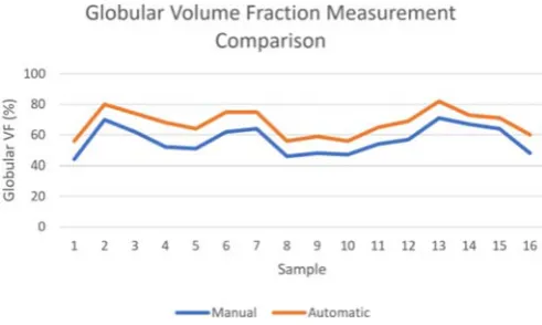
Globular volume fraction is calculated based on the same segmenta-tion used to measure grain size, so can typically be computed in less than a second once grain sizes are already known. The automated mea-surements of the volume fraction of globular alpha initially appeared to be inaccurate, with almost all measurements falling outside the ±10% variation expected, as shown inTable 3. However, on closer inspection the discrepancy between manual and automated measurement was found to be very consistent, with the automated techniques always measuring globular volume fraction higher than the manual methods and this difference usually being approximately 10%. It is also observed that, subsequently, variations in volume fraction between each sample are approximately the same regardless of the measurement techniques being used, as shown inFig. 9. This suggests both manual and auto-mated measurements give meaningful information about the micro-structure but that some form of bias is causing measurements to disagree. A likely cause of this is the difference in how the length and width of grains are selected for measuring aspect ratio. The software fits an ellipse to the grain giving a length and width that are perpendic-ular to each other, with the width representing the widest part of the grain. In manual approaches placing the length and width is done sub-jectively, therefore, length and width may not be perfectly perpendicu-lar and the width measurement may be taken at a narrower section of the grain. This would result in higher aspect ratios for manual measure-ments and a lower percentage of grains being classed as globular, which is what our results show.

Further experiments would be required to investigate this and de-termine which method of measurement gives the true globular volume fraction. However, for developing an automated tool for analysing mi-crostructures the ability to measure the same differences in volume fraction between microstructures as an expert materials scientist would measure is suf_ficient to show our technique provides useful in-formation. Furthermore, due to the predictable effect of bias we can cal-ibrate the software, by reducing all automated measurements taken by 10%, to give results that are consistent between each measurement ap-proach. This allows measurements from manual and automated methods to be compared without the effect of bias. We calibrate the software, rather than the manual measurements, so that all measure-ments are consistent with what would be achieved by an expert mate-rials scientist. However, the subjective nature of manual techniques means we do not know if this is the absolute truth. Further investigation is also required when applying such calibrations in practice, as the ap-propriate calibration level may differ for other datasets. With this cali-bration applied all results are within the expected inter-operator variation, showing the software is capable of matching the measure-ment of expert materials scientists.

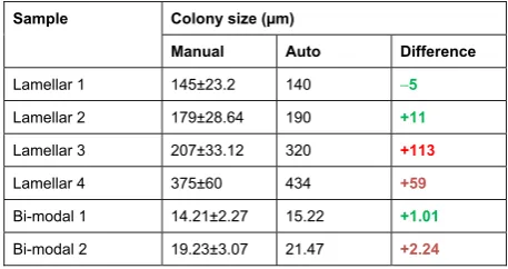
6.2.3. Colony size

Colony size was measured for both lamellar and bi-modal micro-structures and results are shown inTable 4. As manual measurements were taken using linear intercept methods the inter-user variation would be expected to be similar to those for alpha grain sizes. For bi-modal microstructures the variation between measurements was around 1–2μm for 15–20μm colony sizes. This suggests these are also positive results although the disagreement is greater than typically seen for alpha grain measurements. However, for fully lamellar micro-structures the variation ranged from being 5μm for a 145μm colony, to a 133μm difference in a grain manually measured at 207μm. The in-consistency between results is likely because the fully lamellar micro-structures in our dataset contained only a few colonies per image, so any error will have a significant effect on results. Fully lamellar micro-structures quite often contain only a few colonies, and taking hundreds of scans with an SEM is not always practical, so this inconsistency is likely to persist in real world applications of this technique. Therefore, to apply this technique in its current form we must use the visual repre-sentation of segmentation, shown in Fig. 8, to check if colony Table 3

Volume Fraction Measurements of Bi-Modal Microstructures.

Sample Volume fraction of globular alpha (%)

Manual Auto Auto-10%

calibration

Difference

1 44±4.4 56 46 +2

2 70±7 80 70 0

3 62±6.2 74 64 +2

4 52±5.2 68 58 +6

5 51±5.1 64 54 +3

6 62±6.2 75 65 +3

7 64±6.4 75 65 +1

8 46±4.6 56 46 0

9 48±4.8 59 49 +1

10 47±4.7 56 46 −1

11 54±5.4 65 55 +1

12 57±5.7 69 59 +2

13 71±7.1 82 72 +1

14 67±6.7 73 63 −4

15 64±6.4 71 61 −3

16 48±4.8 60 50 +2

Table 4

Colony Size Measurement in Lamellar and Bi-Modal Microstructures.

Sample Colony size (µm)

Manual Auto Difference

Lamellar 1 145±23.2 140 −5

Lamellar 2 179±28.64 190 +11

Lamellar 3 207±33.12 320 +113

Lamellar 4 375±60 434 +59

Bi-modal 1 14.21±2.27 15.22 +1.01

identification is correct. As there are only a few colonies per image it should be easy to spot errors large enough to cause significant problems, and discount or re-measure these images manually. This would not be necessary for our bi-modal microstructures as the larger number of col-onies reduce the statistical significance of errors. Ultimately, however, this is not ideal and these results suggest there are still challenges asso-ciated with colony identi_fication that need to be overcome.

Measurement time for colonies was slower than the methods for globular alpha grains but is still significantly faster than manual mea-surements. The fully lamellar microstructure shown inFig. 8c) was measured in 11.32 s, with similar times required to measure all fully la-mellar microstructures. The measurement time for bi-modal micro-structures was higher with the microstructure shown inFig. 8 a) taking 7 min and 11 s to measure the number of colonies. The significant differences observed in measurement time between fully lamellar and bi-modal microstructures is partly because there were more colonies to detect in the bi-modal microstructures, but also because markers are computed byfirst segmenting the image into a set of smaller gions. This means the algorithm for computing colony markers is re-peated for every region rather than operating once on the full image. This initial segmentation of bi-modal microstructures provides an esti-mate of colony boundaries prior to identifying laths, which is unavail-able in lamellar microstructures. However, the accuracy of these initial boundaries is questionable so it is unclear what benefit this information provides.

Despite the analysis of colonies not obtaining the same standard of results as alpha grain measurement techniques, the techniques can still be used as long as care is taken to visually inspect the segmentation to check they are suitable. Future research will aim to refine this tech-nique to improve its efficiency and reliability. Although we only discuss colony size, it is worth noting that our segmentation also provides infor-mation about the angle of each lath within it. This inforinfor-mation could be used to direct existing techniques for measuring lath widths[13], so that measurements are taken only at angles perpendicular to lath orien-tation rather than at random angles. This could potentially remove lim-itations with these methods, where measurements are only accurate for laths with a high aspect ratio.

6.3. Comparison with existing techniques

We further demonstrate the benefits of our approach by comparing our techniques with the MiPar software developed by Sosa et al.[17]. This software was selected for comparison as, to the authors' knowl-edge, it has the best existing tool for automatically detecting and mea-suring alpha grains in titanium alloys. Colony measurements are not compared here as we know of no existing fully automated approach for this measurement, although some orientation based measurements are possible with the MiPar software. Both MiPar and our techniques were tested on images from our own dataset and images from the dataset provided with the MiPar software. For both techniques, the available parameters were set to give what the operator perceived to be the best result. We found that the MiPar software worked best on Sosa’s microstructures and our methods worked best on our own data, which is unsurprising since each algorithm was design specifically for those datasets. However, some of the microstructures in our study are particularly complex and boundaries are less clearly visible than those in the microstructures MiPar is designed to work with. Segmentation results and subsequent grain measurements for such a microstructure are shown inFig. 10andTable 6respectively. The grain segmentation al-gorithm implemented in MiPar searches for dark pixels in the image which in their data indicates boundaries. However, in our data, dark pixels do not indicate boundaries, therefore, the software will predom-inantly detect noise, causing over-segmentation. Our algorithm mean-while searches not for dark lines but instead for regions of high intensity variations, with the shape of these regions then used to esti-mate grain locations. These features are present in microstructures from both datasets and results in our approach achieving a better result on Sosa_’s microstructures than the MiPar software achieves on ours. This suggests the methods we propose in this paper are more generic and better suited to measuring different types of microstructure, partic-ularly when boundaries are unclear. It should be noted that the MiPar software itself is designed to allow different algorithms to be created and added over time. This test does not represent the ultimate potential of the MiPar software environment but rather the best alpha grain seg-mentation procedure provided at the time of writing1_.

7. Conclusions

We have proposed a new set of image processing techniques capable of automating the measurement of microstructural images. These tech-niques are particularly effective for measuring alpha grain features. In most cases the difference between manual and automated measure-ments using our techniques wasb0.5μm, a particularly strong result given the varied dataset. Measurement of globular volume fraction is also possible, using our techniques. Some calibration was required to give matching results, however, the same difference in globular volume fraction between microstructures was found with or without this. The measurement time for either feature is significantly reduced, from around 15 min per image to a few seconds. Not only will this save money and free up skilled materials scientists to focus on other work, but the time saving is large enough that it would allow larger micro-structural datasets to be analysed than would have previously been Table 5

Summary of measurement accuracy of different features and microstructure.

Grain size Volume fraction of globular alpha Colony size

Good OK Bad Good OK Bad Good OK Bad

Fully globular 100 0 0 – – – – – –

Bi-modal 75 25 0 93 7 0 50 25 25

Lamellar – – – – – – 50 50 0

Fig. 9.Graph showing variations in manual and automatic measurements of globular volume fraction.

1

practical to measure. The automated nature of this approach also means repeatability is achievable, so long as no parameters within the software are changed. Furthermore, the software does not sub-sample grains in the image which typically results in far more grains being measured than using manual approaches, which increases the statistical reliability of results and prevents any potential bias effecting which grains are in-cluded in the sample. These benefits are critical in industry where mate-rials manufacturers require fast results from analysis and for results to be independent from the operator performing the analysis.

Challenges remain with the segmentation of lath colonies. In bi-modal microstructures automated measurements were generally simi-lar to those produced by manual methods, however, were not as good as was achieved for alpha grains. Measurement time was also signifi -cantly longer than for alpha grains, although still faster than manual ap-proaches. Fully lamellar microstructures had inconsistent results with some microstructures achieving accurate measurements and others showing substantial errors. The visualisation of grain boundaries pro-duced by the software should allow for incorrectly measured images to be easily identified and discounted, however, this is not an ideal solu-tion. Further research is currently underway to fully evaluate and im-prove lath segmentation.

Ensuring automated techniques are accurate and robust to varia-tions in microstructure is challenging. We tested our methods on micro-structural images produced by different imaging technologies and of multiple microstructure types, subjected to a variety of thermal and me-chanical processes. The results were mostly positive, confirming our techniques to be capable of measuring a wide variety of microstruc-tures. Comparisons between our techniques and a recent automated

analysis procedure further demonstrated the superior generalisation of our approach. Although tested on microstructures of Ti6Al4V, this generality should allow our method to be applied to a range of different microstructures by changing only a few parameters.

Acknowledgements

This work was supported by Engineering and Physical Sciences Re-search Council through grant EP/I015698/1.

References

[1] G. Lutjering, J.C. Williams, Titanium, Second ed. Springer, 2007.

[2] A. Rosochowski, L. Olejnik, Severe plastic deformation for grain refinement and en-hancement of properties, Microstruct. Evol. Met. Form. Process. (2012) 144. [3] P. Erdely, et al., Design and control of microstructure and texture by

thermomechanical processing of a multi-phase TiAl alloy, Mater. Des. 131 (Oct. 2017) 286–296.

[4] ASTM,“E112 standard test method for determining average grain size.”, 2013. [5] ASTM,“E562 standard test method for determining volume fraction by systematic

manual point cloud.”, 2011.

[6] S.K. Dinda, J.M. Warnett, M.A. Williams, G.G. Roy, P. Srirangam, 3D imaging and quantification of porosity in electron beam welded dissimilar steel to Fe-Al alloy joints by X-ray tomography, Mater. Des. 96 (Apr. 2016) 224–231.

[7] S.A. McDonald, et al., Non-destructive mapping of grain orientations in 3D by labo-ratory X-ray microscopy, Sci. Rep. 5 (1) (Dec. 2015) 14665.

[8] T. Hashimoto, G.E. Thompson, X. Zhou, P.J. Withers, 3D imaging by serial block face scanning electron microscopy for materials science using ultramicrotomy, Ultramicroscopy 163 (Apr. 2016) 6–18.

[9] L. Gillibert, D. Jeulin, 3D Reconstruction and analysis of the fragmented grains in a composite material, Image Anal. Stereol. 32 (2) (Jun. 2013) 107.

[10]Y. Al-Kofahi, W. Lassoued, W. Lee, B. Roysam, Improved automatic detection and segmentation of cell nuclei in histopathology images, IEEE Trans. Biomed. Eng. 57 (4) (Apr. 2010) 841–852.

[11] Q. Zhang, R. Skjetne, Image processing for identification of sea-icefloes and thefloe size distributions, IEEE Trans. Geosci. Remote Sens. 53 (5) (May 2015) 2913–2924. [12]K.H. Moon, A.C. Falchetto, J.H. Jeong, Microstructural Analysis of Asphalt Mixtures

Using Digital Image Processing Techniques, 2013.

[13] P. Collins, B. Welk, T. Searles, J. Tiley, J. Russ, Development of methods for the quan-tification of microstructural features inα+β-processedα/βtitanium alloys, Mater. Sci. Eng. A 508 (1) (2009) 174–182.

[14]J. Tiley, T. Searles, E. Lee, S. Kar, R. Banerjee, Quantification of microstructural fea-tures inα/βtitanium alloys, Mater. Sci. Eng. A 372 (1) (2004) 191–198. Fig. 10.Segmentation comparison between our methods and MiPar software where a) and d) are an original image from each dataset, b) and e) is the segmentation by MiPar and c) and f) is the segmentation by our method. (For interpretation of the references to colour in thisfigure legend, the reader is referred to the web version of this article.)

Table 6

Comparison between MiPar and our technique.

Manual measurement

MiPar measurement

Our measurement

[15] D. Yang, Z. Liu, Quantification of microstructural features and prediction of mechan-ical properties of a dual-phase Ti-6Al-4V alloy, Materials (Basel) 9 (8) (2016) 1–14. [16] J. Zhe, Y. He, H. Li, X. Fan, A new method for separating complex touching equiaxed and lamellar alpha phases in microstructure of titanium alloy, Trans. Nonferrous Metals Soc. China 23 (8) (2013) 2265–2269.

[17]J. Sosa, D. Huber, B. Welk, H. Fraser, Development and application of MIPAR™: a novel software package for two-and three-dimensional microstructural characteri-zation, Integr. Mater. Manuf. Innov. 3 (1) (2014) 10.

[18] I. Polmear, Light Alloys; From Traditional Alloys to Nanocrystals, Butterworth-Heinemann, 2005.

[19]A. Chokshi, A. Rosen, J. Karch, H. Gleiter, On the validity of the hall-petch relation-ship in nanocrystalline materials, Scr. Metall. 23 (10) (1989) 1679–1683. [20] H. Liu, H. Sun, B. Liu, D. Li, F. Sun, X. Jin, An ultrahigh strength steel with ultrafi

ne-grained microstructure produced through intercritical deformation and partitioning process, Mater. Des. 83 (Oct. 2015) 760–767.

[21] L. Liu, et al., Ultrafine grained Ti-based composites with ultrahigh strength and duc-tility achieved by equiaxing microstructure, Mater. Des. 79 (Aug. 2015) 1–5. [22] C.R. Gonzalez, R. Woods, Digital Image Processing, Pearson Educ., 2002

[23] P. Salembier, J. Serra, Flat zonesfiltering, connected operators, andfilters by recon-struction, IEEE Trans. Image Process. 4 (8) (1995) 1153–1160.

[24] H. Sun, J. Yang, M. Ren, A fast watershed algorithm based on chain code and its ap-plication in image segmentation, Pattern Recogn. Lett. 26 (9) (Jul. 2005) 1266–1274. [25] P. Soille, Morphological Image Analysis: Principles and Applications, 2013. [26] S. Beucher, F. Meyer, The Morphological Approach to Segmentation: The Watershed

Transformation, Opt. Eng. York-Marcel, 1992.

[27]M. Kass, A. Witkin, D. Terzopoulos, Snakes: active contour models, Int. J. Comput. Vis. 1 (4) (1988) 321–331.

[28] J. Serra, Introduction to mathematical morphology, Comput. Vis. Graph. Image Pro-cess. 35 (3) (1986) 283–305.

[29] G. Coleman, H. Andrews, Image segmentation by clustering, Proc. IEEE 67 (5) (1979) 773–785.

[30]P. Murray, S. Marshall, A new design tool for feature extraction in noisy images based on grayscale hit-or-miss transforms, IEEE Trans. Image Process. 20 (7) (Jul. 2011) 1938–1948.

[31]Y. Zheng, B. Jeon, D. Xu, Q. Wu, Image segmentation by generalized hierarchical fuzzy C-means algorithm, J. Intell. Fuzzy Syst. 28 (2) (2015) 961–973.

[32] F. Meyer, Topographic distance and watershed lines, Signal Process. 38 (1) (1994) 113–125.

[33]P. Singhai, S. Ladhake, Brain tumor detection using marker based watershed seg-mentation from digital mr images, International Journal of Innovative Technology and Exploring Engineering (IJITEE) ISSN 2013, pp. 2278–3075.

[34]X. Zhang, F. Jia, S. Luo, G. Liu, Q. Hu, A marker-based watershed method for X-ray image segmentation, Comput. Methods Prog. Biomed. 113 (3) (2014) 894–903. [35] D. Li, G. Zhang, Z. Wu, L. Yi, An edge embedded marker-based watershed algorithm

for high spatial resolution remote sensing image segmentation, IEEE Trans. Image Process. 19 (10) (2010) 2781–2787.

[36]E. Breen, R. Jones, Attribute openings, thinnings, and granulometries, Comput. Vis. Image Underst. 64 (3) (1996) 377–389.

[37] L. Li, J. Yao, J. Tu, X. Lu, K. Li, Y. Liu, Edge-based split-and-merge superpixel segmen-tation, Autom. IEEE International Conference on 2015 Aug 8, pp. 970–975 IEEE. [38]I. Manousakas, P. Undrill, G. Cameron, Split-and-merge segmentation of magnetic

resonance medical images: performance evaluation and extension to three dimen-sions, Comput. Biomed. Res. 31 (6) (1998) 393–412.

[39] D. Ballard, CM Brown Computer Vision, NY Prentice Hill, 1982.