Mean flow evolution of saturated forced shear flows in polytropic atmospheres

City, University of London Institutional Repository

Citation

:

Witzke, V. and Silvers, L. J. (2019). Mean flow evolution of saturated forced

shear flows in polytropic atmospheres. EAS Publications Series, 82, pp. 259-269. doi:

10.1051/eas/1982026

This is the accepted version of the paper.

This version of the publication may differ from the final published

version.

Permanent repository link:

http://openaccess.city.ac.uk/id/eprint/16002/

Link to published version

:

http://dx.doi.org/10.1051/eas/1982026

Copyright and reuse:

City Research Online aims to make research

outputs of City, University of London available to a wider audience.

Copyright and Moral Rights remain with the author(s) and/or copyright

holders. URLs from City Research Online may be freely distributed and

linked to.

City Research Online:

http://openaccess.city.ac.uk/

[email protected]

arXiv:1611.10131v1 [astro-ph.SR] 30 Nov 2016

EAS Publications Series, Vol. ?, 2016

MEAN FLOW EVOLUTION OF SATURATED FORCED

SHEAR FLOWS IN POLYTROPIC ATMOSPHERES

V. Witzke

and L. J. Silvers

Abstract. In stellar interiors shear flows play an important role in many physical processes. So far helioseismology provides only large-scale measurements, and so the small-scale dynamics remains insufficiently understood. To draw a connection between observations and three-dimensional DNS of shear driven turbulence, we investigate horizon-tally averaged profiles of the numerically obtained mean state. We fo-cus here on just one of the possible methods that can maintain a shear flow, namely the average relaxation method. We show that although some systems saturate by restoring linear marginal stability this is not a general trend. Finally, we discuss the reason that the results are more complex than expected.

1

Introduction

The complex gas dynamics present in stellar interiors is important for many stel-lar process, such as mixing behaviour (see e.g. Zahn, 1974; Schatzman, 1977) and magnetic field generation (e.g. Miesch and Toomre, 2009; Jones et al., 2010). The tachocline, which is located at the base of the convection zone, is believed to play a crucial role in these processes. This thin region with a strong radial shear flow was theoretically predicted (Spiegel and Zahn, 1992) and subsequently confirmed by helioseismic observations (e.g. Kosovichev, 1996).

Velocity measurements obtained by helioseismology suggest a hydrodynami-cally stable tachocline (Miesch, 2007) i.e. the approximated Richardson number is significantly greater than the theoretical stability threshold of 1/4 (Miles, 1961). However, helioseismology is restricted to large-scale time-averaged measurements (Christensen-Dalsgaard and Thompson, 2007), such that turbulent motions can still be present on small length- and time-scales. Such a scenario, where a hy-drodynamically unstable system appears stable on large scales was, for example,

1

Department of Mathematics, City University of London, Northampton Square, London, EC1V 0HB, UK

c

2 Title : will be set by the publisher

suggested by Vasil and Brummell (2009) and remains to be investigated.

Due to the inability of observing most astrophysical shear regions in detail, ana-lytical and numerical techniques have to be used to investigate the motions present in such regions. Most local numerical studies of shear flows that lead to turbulence exploit an unforced flow (e.g. Caulfield and Peltier, 2000; Smyth and Winters, 2003), which results in a finite lifetime of an initially unstable background state. However, astrophysical shear flows can be either transient features or be sustained over very long time-scales. Thus investigations of astrophysical shear flows use different methods to reach a sustained flow. While we previously have compared various methods to sustain large-scale shear flows during the saturated phase (see Witzke et al., 2016) here we concentrate on just one method. The method se-lected, the relaxation method, is suitable for modelling a target flow in the satu-rated phase. This method allows the time-scale on which the system is driven to the initial shear flow to be adjusted. Through our investigations we shed light on the question of how likely it is that an initially unstable shear flow will result in global flow profiles that suggest a stable system. We analyse the saturated regime of two differently stratified systems in terms of their horizontally averaged profiles and the resulting effective Richardson number.

2

Model

We consider a three-dimensional domain of depth d, bounded by two horizontal planes located at z = 0 and z = 1, and periodic in both horizontal directions. The fluid is assumed to be an ideal monatomic gas with the adiabatic index

γ = cp/cv = 5/3 and constant transport coefficients. The set of dimensionless equations describing the problem and the forcing method used to sustain an ini-tial velocity,u0= (u0(z),0,0)T, are exactly the same as described in Witzke et al.

(2016).

In order to investigate whether an initially unstable system can reach a sat-urated state where the horizontally averaged profiles, associated with large-scale averaged measurements, suggest a stable system we focus on two differently strat-ified cases. Case I is strongly stratstrat-ified, but the polytropic index is chosen such that it is not far from being unstable to convection. This case was investigated in Witzke et al. (2016), where different forcings were compared. Here rather than focusing on the different forcing methods we will instead examine the horizontally averaged profiles during the saturated regime in order to understand if it suggests a stable or unstable system. Case II is weakly stratified, but has a large polytropic index to ensure that the system is far from the onset of convection. The Prandtl number is takenσ = 0.1 for both cases, as σ <1 is more relevant for stellar in-teriors. All relevant parameters are summarised in Table 1. Using the relaxation method we consider different relaxation times,τ0, in order to investigate how

Table 1.Parameters for the investigated cases, where the resolution of the domain is given by Nx, Ny and Nz. The dynamical viscosity is Ckσ, where Ck is the thermal

diffusivity and σ the Prandtl number. The temperature gradient is denoted by θ and the polytropic index is m. For the initial velocity profile the shear amplitude isU0 and

the shear width is controlled byL_{u. The resulting minimum Richardson number,}Ri_{, is}

calculated for the initial state.

Case Ckσ θ m U0 1/Lu Nx Ny Nz Ri Case I 10−4 5 1.6 0.2 80 256 256 360 0.003

Case II 10−5 0.25 4 0.05 40 256 64 384 0.07

3

Results

During the evolution of an unstable shear flow the horizontally averaged density, temperature and velocity profiles are modified. Therefore, the effective minimalRi

number of the system changes. In stratified systems this modification comes from two sources: The change in the Brunt-V¨ais¨al¨a frequency, due to changes in the averaged density and temperature profiles, and the change in turnover rate of the shear. For both cases we consider the first contribution remains small compared with the latter one. The minimal effective Richardson number is calculated from the horizontally averaged profiles as follows,

minRief f = min   

−θ(m+ 1)

_∂u¯(z) ∂z

2 _γ

−1

¯

ρ(z)

∂ρ¯(z)

∂z + γ

¯

T(z)

∂T¯(z)

∂z

 

, (3.1)

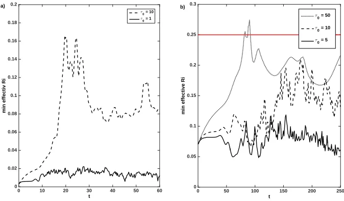
where horizontally averaged quantities are denoted by an overbar. This quantity is compared to the initial minimal Ri in order to study the change to the system. InvestigatingRief f for case I (see Fig. 1 (a)), we find that it increases significantly and reaches a maximum when the instability saturates. Afterwards,Rief f fluctu-ates around a value, and this value increases asτ0 increases. The late time values

are Rief f ≈ 0.09 for the relaxation method withτ0 = 10 andRief f ≈0.01 for

τ0= 1.0. For both runs of case I,Rief f obtained in the statistically steady state is one order of magnitude greater than the initialRi= 0.003 number.

For case II, see Fig. 1 (b), the system is initially closer to the stability threshold. Varying the relaxation time gives rise to a similar trend as in case I, where the ef-fective Richardson number during the quasi-static regime increases asτ0increases.

4 Title : will be set by the publisher

0 10 20 30 40 50 60

t

0 0.02 0.04 0.06 0.08 0.1 0.12 0.14 0.16 0.18 0.2

min effectiv Ri

a)

τ

0 = 10

τ

0 = 1

0 50 100 150 200 250

t

0 0.05 0.1 0.15 0.2 0.25 0.3

min effective Ri

b)

τ

0 = 50

τ

0 = 10

τ

0 = 5

Fig. 1.The minimal effective Richardson number obtained from the horizontally aver-aged profiles as in Equation (3.1) with time for each of the two cases we consider. a) case I using two different relaxations timesτ0is displayed. b) case II with three different

relaxation timesτ0 is shown. The red line indicates the 1/4 stability threshold.

4

Conclusions

Investigating a shear flow instability after the system starts saturating reveals a significant increase in the minimal Ri obtained from horizontally averaged pro-files. It becomes evident that the relaxation time used in the forcing method has a significant effect on the resulting minimalRief f during the steady state. Starting with an initially unstable configuration close to the stability threshold can lead to a transient phase where the effective Ri number becomes greater than 1/4. However, the minimal Rief f decreases notably below the stability threshold at later times. It is therefore difficult to achieve a turbulent flow that looks stable in a pure hydrodynamical system with a connectively stable stratification when starting from an initially unstable configuration.

Acknowledgements

References

Caulfield, C. P. and Peltier, W. R.: 2000, J. Fluid Mech.413, 1

Christensen-Dalsgaard, J. and Thompson, M. J.: 2007, in D. W. Hughes, R. Rosner, and N. O. Weiss (eds.), The Solar Tachocline, pp 53–86, Cambridge University Press

Jones, C. A., Thompson, M. J., and Tobias, S. M.: 2010, Space Sci. Rev. 152(1-4), 591

Kosovichev, A. G.: 1996, ApJL 469, L61

Miesch, M. S.: 2007, in D. W. Hughes, R. Rosner, and N. O. Weiss (eds.), The Solar Tachocline, pp 109–128, Cambridge University Press

Miesch, M. S. and Toomre, J.: 2009, Annu. Rev. Fluid Mech.41, 317

Miles, J. W.: 1961, J. Fluid Mech.10, 496

Prat, V. and Ligni`eres, F.: 2014, A&A 566, A110

Schatzman, E.: 1977, A&A 56, 211

Smyth, W. D. and Winters, K. B.: 2003, J. Phys. Oceanogr. 33, 694

Spiegel, E. A. and Zahn, J.-P.: 1992, A&A 265, 106

Vasil, G. M. and Brummell, N. H.: 2009, ApJ 690, 783

Witzke, V., Silvers, L. J., and Favier, B.: 2016, MNRAS 463, 282

Zahn, J.-P.: 1974, in P. Ledoux, A. Noels, A. Rodgers, I. A. Union, I. A. U. C. 27, and I. A. U. C. 35 (eds.),Stellar Instability and Evolution, Springer