Abstract: Choice set generation is a challenging aspect of disaggregate level residential location choice modelling due to the large number of candidate alternatives in the universal choice set (hundreds to hundreds of thousands). The classical Manski method (Manski, 1977) is infea-sible here because of the explosion of the number of posinfea-sible choice sets with the increase in the number of alternatives. Several alternative ap-proaches have been proposed in recent years to deal with this issue, but these have limitations alongside strengths. For example, the Constrained Multinomial Logit (CMNL) model (Martínez et al., 2009) offers gains in efficiency and improvements in model fit but has weaknesses in terms of replicating the Manski model parameters. The rth-order Constrained Multinomial Logit (rCMNL) model (Paleti, 2015) performs better than the CMNL model in producing results consistent with the Manski model, but the benefits disappear when the number of alternatives in the universal choice set increases. In this study, we propose an improved CMNL model (referred to as Improved Constrained Multinomial Logit Model, ICMNL) with a higher order formulation of the CMNL penalty term that does not depend on the number of alternatives in the choice set. Therefore, it is expected to result in better model fit compared to the CMNL and the rCMNL model in cases with large universal choice sets. The performance of the ICMNL model against the CMNL and the rCMNL model is evaluated in an empirical study of residential location choices of households living in the Greater London Area. Zone level models are estimated for residential ownership and renting decisions where the number of alternatives in the universal choice set is 498 in each case. The performance of the models is examined both on the esti-mation sample and the holdout sample used for validation. The results of both ownership and renting models indicate that the ICMNL model performs considerably better compared to the CMNL and the rCMNL model for both the estimation and validation samples. The ICMNL model can thus help transport and urban planners in developing better prediction tools.
Keywords: Choice set generation, Manski model, constrained multi-nomial logit model, Greater London
Modelling residential location choices with implicit availability of
alternatives
Article history:
Received: August 16, 2018 Received in revised form: January 14, 2019
Accepted: March 3, 2019 Available online: July 24, 2019
Copyright 2019 Md Bashirul Haque, Charisma Choudhury, & Stephane Hess
http://dx.doi.org/10.5198/jtlu.2019.1450
ISSN: 1938-7849 |Licensed under the Creative Commons Attribution – Noncommercial License 4.0
The Journal of Transport and Land Use is the official journal of the World Society for Transport and Land Use (WSTLUR) and is published and sponsored by the University of Minnesota Center for Transportation Studies.
Md Bashirul Haque University of Leeds [email protected] and
Shahjalal University of Science and Technology
Charisma Choudhury University of Leeds
1
Introduction
Home location and urban environment determine the activities and travel patterns of individual house-hold members. For example, househouse-holds living in inner-city areas with closer proximity to facilities tend to travel shorter distances, make more non-motorized trips and are found to be less car-dependent for local transport than suburbanites (Næss, 2009). These prevailing dynamics and interactions among resi-dential location, urban form and travel behaviour are at the heart of integrated land use and transport planning. Therefore, modelling residential location choice is a key component of integrated planning.
Modelling of residential location choices has numerous challenges from both a methodological and empirical standpoint. A key issue in this regard is choice set formulation, which has a substantial effect on the model outputs (Swait, 2001; Bell, 2007). In a standard choice model, an analyst needs to specify all the alternatives considered by the decision makers. However, in the context of residential location choice modelling, typically the individual-level choice set is unknown to the analyst and the universal choice set is very large – hundreds in case of zone level to hundreds of thousands in the case of dwelling level models. A review of the literature reveals several residential location choice models where the uni-versal choice set has been used as the individual choice set (e.g., Bhat & Guo, 2004; Zolfaghari, 2013; Haque, Choudhury, & Hess, 2018).
Considering the universal choice set for individuals is however also behaviourally unrealistic, as in the real world, households are neither aware of the full set of alternatives nor consider all alternatives they are aware of. Different households might thus have different consideration sets based on household preferences and sociodemographic characteristics, as well as their knowledge of available alternatives. For example, a household may not consider an alternative if they do not have enough knowledge about it or if the alternative is very far from the workplace of a household member. Therefore, it is expected that better ways to model the choice set will make the models behaviourally more representative. This, in turn, will lead to more accurate models for planning and policy making.
Modelling of individual choice sets from a large universal choice set (e.g., disaggregate level resi-dential location choice modelling) using the two-stage probabilistic approach (e.g., Manski 1977; Swait & Ben-Akiva, 1987, etc.) is infeasible due to the explosion of estimation complexity with increasing numbers of alternatives in the universal choice set. Therefore, a two-stage deterministic approach has been used in several studies where a limited set of alternatives have been screened from a universal choice set for each individual based on some behavioural rules (e.g., Farooq & Miller, 2012; Rashidi, Auld, & Mohammadian, 2012; Zolfaghari, 2013, etc.). However, this technique has a high risk of excluding potentially viable alternatives from the individual choice set and including irrelevant alternatives. The performance of the deterministic choice set generation approaches has been evaluated and criticized in the literature (Zolfaghari, 2013). A single-stage semi-compensatory technique (e.g., Cascetta & Papola, 2001, 2009: Murtinez, Aguila, & Hurtubia, 2009; Paleti, 2015) provides an alternative approach to avoiding the risk of screening of alternatives in the two-stage deterministic approaches. This approach captures the individual choice set implicitly through a form of utility penalization and is computation-ally feasible in the case of large universal choice sets. However, semi-compensatory methods also have limitations in their ability to reproduce the true parameters in estimation (Bierlaire, Hurtubia, & Flöt-teröd, 2010).
Motivated by these points, the specific objectives of this study are as follows:
• to evaluate the performance of state-of-the-art semi-compensatory choice set generation tech-niques in the context of residential location choice modelling;
• to investigate the potential to improve choice set generation techniques without compromising computational tractability; and
• to investigate the existence of underlying heterogeneity in the choice set of long-term and medi-um-term residential location choices (residential ownership and renting respectively).
In the next two sections, we review the choice set generation techniques in further detail and pro-pose an improved choice set generation technique. The data for our empirical example is presented next followed by the estimation and the validation results. We conclude with a summary of the findings and directions for future research.
2
Review of choice set generation techniques
The two-stage probabilistic approach proposed by Manski (1977) is a classical solution for modelling individual choice sets. This method requires the estimation of probabilities of all possible choice sets in the first stage and the conditional probabilities of alternatives across all choice sets in the second stage. Both stages are estimated simultaneously. The number of possible choice sets explodes with the number of alternatives in the universal choice set. For J alternatives, the number of possible choice sets is 2J-1. Therefore, this method is computationally infeasible for a medium to large choice set (e.g., residential location choice, route choice, destination choice, etc.).
The unconditional probability of choosing an alternative by a decision maker in the Manski meth-od is the prmeth-oduct of the conditional probability of the alternative (given the choice set) and the prob-ability of the choice set. The probprob-ability can be presented as follows:
Pin (C)=∑Cs∊C Pn (i/Cs )×P(Cs ) (1)
where Pin (C) is the unconditional probability of choosing alternative i by individual n from universal set C, Pn (i/Cs ) is the conditional probability of choosing alternative i from the choice set Cs (Cs∊C) and
P(Cs ) is the probability of the choice set being Cs . We thus have a sum across all the possible choice sets. Other probabilistic approaches proposed in the literature as alternatives to the Manski method (e.g., Swait & Ben-Akiva, 1987; Swait, 2001; Kaplan, Bekhor, & Shiftan, 2011; Zolfaghari, 2013; Bhat, 2015, etc.) also have computational issues for large numbers of alternatives.
The typical approach in the literature for modelling with large universal choice sets is random selec-tion of a subset of alternatives from the universal choice set (Bhat & Guo, 2007; Habib & Miller, 2009; Lee & Waddell, 2010; Guevara, 2010). This approach reduces the computational burden substantially and can also produce consistent parameters in estimation if households consider all alternatives in the universal choice set (McFadden, 1978). This is, however, a poor assumption in the case of disaggre-gate level residential location choice modelling. Rather, it seems more reasonable that households apply behavioural process heuristics for screening of the alternatives (Bhat, 2015). Ignoring this underlying search mechanism can potentially lead to inaccurate parameter estimation, wrong model forecasts and inappropriate policy implications (Kwan & Hong, 1998; Arentze & Timmermans, 2005).
the individual choice set when certain attributes of an alternative exceed exogenous thresholds. These exogenous thresholds can be either imposed deterministically based on insights from the data (Farooq & Miller, 2012) or can be computed (Zolfaghari, 2013). Importance sampling techniques have also been used in the context of residential location choice modelling (e.g., Rashidi et. Al, 2012; Zolfaghari, 2013, etc.). These techniques are similar to the deterministic constraint-based approaches but allow propor-tional sampling of alternatives from within and outside the threshold zone. For example, Farooq and Miller (2012) applied importance sampling to construct individual choice sets for residential location choice modelling by taking 75% of alternatives within 15 km of the past location and the remaining 25% from outside the threshold. Since these techniques are based on assumptions made by the analyst, there is a high risk of choice set misspecification and consequently, poor model fit and biased parameter estimation.
Heuristic-based semi-compensatory approaches can avoid the combinatorial number of choice sets in the probabilistic approach and the risk of elimination by aspect approaches (e.g., ignoring alternatives that have non-zero choice probabilities), and therefore become appealing in case of modelling with a large universal choice set. The basic principle of these methods is the adjustment of systematic utility based on the probability of an alternative being in the individual choice set. A penalty term is introduced in the utility equation for the adjustment. Therefore, the utility function for alternative i and person n can be defined as follows:
Uin= Vin+ln(ϕin )+ɛin where 0≤ϕin≤1 (2)
where ϕin is the probability of alternative i being in the choice set of individual n, Vin is the deterministic utility of the alternative i for individual n and ɛin is the usual identically and independently distributed (iid) extreme value error term. If there is a full probability of an alternative being in the individual choice set, the penalty term becomes zero (i.e., no adjustment is required).
Different functional forms of ϕin have been used in different semi-compensatory approaches. ϕin is expressed as a binary logit function of attributes related to choice set formation in the Implicit Avail-ability Perception Random Utility (IAPRU) model proposed by Cascetta and Papola (2001). The math-ematical expression of ϕin is as follows:
(3)
where zik is a parameter associated with attribute k and alternative i and µk is the scale parameter. Second order utility penalization is also proposed based on the Taylor series expansion for further utility cut-off of less attractive alternatives (Cascetta & Papola, 2001). This method, however, leads to estimation difficulties in complex specifications with multiple constraints. Moreover, second order utility penaliza-tion has convergence issues if a chosen alternative is subjected to an extreme penalty. For example, if commute distance is considered as an availability/perception attribute (k) in residential location choice modelling and the penalty parameter (µk ) is 0.8, the utility cut-off for an alternative 10 km away from the individual workplace is 1498 units, leading to a choice probability close to zero. If that alternative is chosen by anyone (which is possible in reality if the alternative is attractive in terms of all other at-tributes), it can lead to estimation problems.
or multiple attributes). An alternative j is worse than i if quality attributes Qi (i.e., attributes with posi-tive coefficients) are smaller in j than in i and cost attributes Ci (i.e., attributes with negative coefficients) are larger in j than in i, with at least one inequality strictly satisfied. This framework, however, does not account for how worse one alternative is compared to another alternative. The rule of dominance can be expressed as follows:
(4)
indicates that alternative j is dominated by alternative i for individual n if inequality criteria is satisfied for at least one attribute. The penalty term can be expressed as follows:
(5)
The constrained multinomial logit model (CMNL) proposed by Martínez et al. (2009) has greater flexibility to accommodate multiple constraints with exogenous bounds (both upper and lower) to simulate the individual choice set implicitly. A binary logit functional form is also considered here to es-timate the probability of alternatives being in the individual choice set (ϕin). The binary logit functional form of ϕin with an upper threshold tnk on a constrained attribute k can be presented as follows:
(6)
(7)
where zik is the value of constrained attribute k, tnk is the threshold of attributes k for individual n, ηk is the cut off tolerance (proportion of decision makers violating the threshold) and µk is the scale pa-rameters (µk>0). ϕink collapses to 1 and ηk under the conditions (zik-tnk)=-∞ and zik=tnk, respectively. If a constraint is applied on multiple attributes, the total penalty term becomes
(8)
Paleti (2015) proposed the rth-order CMNL model (called rCMNL) where the complexity is linear
with the size of the choice set. A higher order functional form of the CMNL penalty term (ϕin) is pro-posed in this regard. The rth-order penalty in rCMNL is the natural logarithm of the following rth- order
expressions.
(9)
(10)
(11)
(12)
Where is is the probability of choosing alternative i from the full choice set without any penalization. (13)
Using synthetic data and real-world data, the author demonstrates that higher order penalization performs considerably better than the CMNL model in terms of replicating the Manski model pa-rameters. However, in both examples, the number of alternatives in the universal choice sets was very limited (three and five alternatives, respectively). If the number of alternatives in the choice increases, the probability of each alternative is likely to go down. For a very large universal choice set (hundreds to thousands of alternatives), will be too small and (i.e., the model collapses to the first order CMNL).
3
Improved constrained multinomial logit model (ICMNL)
Though the complexity of the CMNL model remains linear with an increase in the number of alterna-tives in the choice set, it struggles to replicate the outcomes of the Manski method (Bierlaire, Hurtubia, & Flötteröd, 2010). The penalty term considered in the CMNL model is a first order penalty derived from the attributes that influence individual choice sets. The higher order utility penalization proposed in the rCMNL model can minimize the error in the CMNL model outcomes when the size of the uni-versal choice set is small. In case of a large uniuni-versal choice set, the higher order penalty in the rCMNL model collapses to the first order CMNL penalty and cannot offer any further improvement. This is due to the fact that the rCMNL penalty depends on the probability of choosing alternatives from the uni-versal choice set which is likely to be very small for large uniuni-versal choice sets. We therefore propose an alternate formulation of higher order approximation of the availability term (ϕin) in the CMNL model based of the concept of a Taylor series expansion which is independent of the number of alternatives in the universal choice set. This is motivated by the application of Taylor series expansion in the context of the Implicit Availability Perception (IAP) logit model (see Cascetta & Papola, 2001, for details). The basic utility equation with implicit availability of alternatives can be expressed as follows: (14)re-searcher’s assumptions, the estimated value of the implicit availability term (ϕin) is unlikely to be the true value. Therefore, in the ICMNL model, we have decomposed the availability into expected availability and an error term. Thus, the true penalty can be expressed as ln(ϕin)=E( ln(ϕin))+δin where δin is the er-ror term (divergence between true and expected penalty). The utility equation can be revised as follows
(15)
For simplicity, the total error (τin) is assumed to be independently and identically distributed (IID). Based on the 2nd order Taylor series expansion, the expected penalty can be expressed as below
(16)
Since the distribution of ϕin is unknown, the variance of ϕin is also unknown. Considering the variance of the Bernoulli distribution, Var (ϕin )=ϕin (1-ϕin) , the equation (16) can be modified as follows
(17)
The utility equation (15) can be presented as follows
(18)
is the second order utility penalty where
(19)
The average availability ϕin can be estimated implicitly using the mathematical formulation proposed in the CMNL model (see equation 6). A constraint is applied to the attributes related to the alternative to estimate the choice set probability of the alternative. If the constraint is applied on multiple attributes, the total penalty becomes:
(20)
(21)
and the log likelihood function is
(22)
where yin = 1 if alternative i is chosen by household n and yin = 0 for all nonchosen alternatives. The maxi-mum likelihood estimates of the model parameters are found by maximizing this function. Functional forms used in different methods are explained in the following sections.
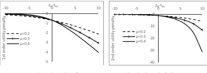
If the attributes move away from the bound, the rate of increment of 2nd order penalties in ICMNL
become considerably stronger than the 1st order penalty. For example, for µ=0.4, if the value of (zik - tnk) moves from 5 to 10, the increment of the first-order penalty is 2 units which is 25 units for second order penalty (Figure 1). Therefore, the first order penalty is considered as a soft penalty and the second order penalty is considered as a hard penalty. The scale parameter also determines the size of the penalty.
[image:8.612.99.512.304.451.2](a) 1st order penalty (soft) (b) 2nd order penalty (hard)
Figure 1. Penalization of the utility function
Due to applying hard penalties on those alternatives that are unlikely to be in the individual choice set, the choice probabilities of these alternatives tend to zero which is behaviourally reasonable. There-fore, the ICMNL model is expected to be a better approximation of the Manski formulation. The performance of the ICMNL is first evaluated here with a simple analysis (similar to that in Bierlaire, Hurtubia, & Flötteröd, 2010). For this analysis, only two alternatives are considered where alternative 1 is always available in the choice set (ϕ1=1) and alternative 2 has a probability of being in the choice set (ϕ2≤1). This hypothesis is similar to the CMNL concept where alternatives within a threshold are always available in the choice set and choice set membership probabilities are assigned for those alternatives that are outside the threshold zone. In the CMNL, rCMNL, and ICMNL, the probability of choosing alternative 1 is as follows:
(23)
where V1 and V2 are the systematic utilities of alternatives 1 and 2, respectively.
The mathematical formulation of penalty terms in the CMNL, rCMNL and ICMNL models can thus be summarized as follows:
(25)
(26)
(27)
The probability of choosing alternative 1 based on the Manski formulation is as follows:
(28)
where P(C[1]) and P(C[1,2]) are the probabilities of choice sets containing alternative 1 only and both of the alternatives (1 and 2), respectively. The probability of a given choice set can be expressed as follows (Bierlaire, Hurtubia, & Flötteröd 2010).
(29)
(30)
(31)
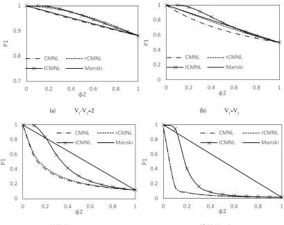
The choice probability of alternative 1 (P1) is calculated for different values of ϕ2 (probability of alternative 2 being in the choice set) under different conditions using the CMNL, rCMNL, ICMNL and Manski formulation presented above. The results are plotted in Figure 2.
• Under condition (a) when the utility of alternative 1 (V1) is larger than the utility of alternative 2, the semi-compensatory approaches (CMNL, rCMNL and ICMNL model) can replicate the Manski model probability quite well though the CMNL model gives the best fit (Figure 2a). • Under condition (b) when the utility of both of the alternatives is the same or close to each
other, CMNL, rCMNL and ICMNL model can still offer a close approximation to the Manski method though rCMNL model results in the best fit (Figure 2b).
• The main concerns are conditions (c) and (d), when the utility of alternative 1 is smaller than alternative 2. In these cases, the semi-compensatory approaches cannot reproduce the Manski model results and the error produced by the semi-compensatory approaches becomes larger with the decrease of the utility of alternative 1 (also demonstrated by Bierlaire, Hurtubia, & Flötteröd, 2010). However, the ICMNL model can considerably reduce the error between the Manski and the CMNL model (Figures 2c and 2d).1,2
1 ICMNL model has asymmetric domains of under-estimating and over-estimating the Manski model probabilities. The
asym-metric property of under and overestimation depends on the differences in the utility of the alternatives. Since the ICMNL model can reduce the error considerably compared to the CMNL and the rCMNL models (Figure 2c and 2d), this asymmetric property is unlikely to affect the model performance.
(a) V1-V2=2 (b) V1=V2
[image:10.612.100.509.85.409.2](c) V1-V2=-2 (d) V1-V2=-4
Figure 2. Choice probability of alternative 1 for different utility differences
4
Data analysis and variable specification
The London Household Survey Data (LHSD) collected in 2002 is considered as the primary data source for this study. This dataset contains detailed information about the socio-demographic character-istics (household size, income, etc), dwelling charactercharacter-istics (tenure type, size, price/rent, etc.), employ-ment status, home and work location, car ownership, etc of 8,158 households from the Greater London Area (GLA). The dataset contains information of 4,491 households living in occupier-owned houses, 2,489 households living in houses rented from councils or housing authorities, 1,087 households living in privately rented houses and 91 households living in shared accommodation. Since this study only considered households that live in owned or privately rented houses, have at least one working member and had at least one residential move within the GLA, the final dataset contains information from 1,875 owners and 382 renters.
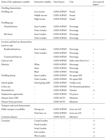
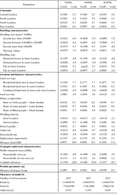
Table 1. Parameters considered for this study
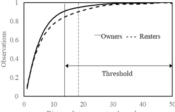
Not surprisingly, statistical analysis of the data shows that households are inclined to choose residential location alternatives close to their current home. However, owners’ preferences to relocate near to their current home are found to be stronger than those of renters (Figure 3). For example, 90% owners chose their new locations within 14 km of their past homes and for the remaining 10%, they are spread be-tween 14 and 50km whereas 90% renters chose their new locations within 18 km of their past homes
Name of the explanatory variables Interaction variables Data Sources Unit Anticipated impact Dwelling characteristics
Dwelling cost Low income LHSD &WAD Pound
-Middle income LHSD &WAD Pound
-High income LHSD &WAD Pound
-Dwelling type
Detached house Inner London LHSD &WAD Percentage
-Outer London LHSD &WAD Percentage
Flat house Inner London LHSD &WAD Percentage +
Outer London LHSD &WAD Percentage
-Location and land use characteristics Land use type
Residential land use Inner London LHSD &WAD Percentage +
Outer London LHSD &WAD Percentage +
Commercial land use - LHSD &WAD Percentage
-Land use mix - LHSD &WAD Index varies from 0 to 1 +
Ethnicity White LHSD &WAD Percentage +
Asian LHSD &WAD Percentage +
Black LHSD &WAD Percentage +
Dwelling density Inner London LHSD &WAD Per square KM
-Outer London LHSD &WAD Per square KM -School quality School going child LHSD &WAD Unitless score +
Crime rate - LHSD &WAD Per thousand population
-Household size - LHSD &WAD Number
+/-Employment opportunity - LHSD &WAD Per person +
Distance from CBD - LHSD <S Kilometre +
Distance from past home - LHSD <S Kilometre
-Transport and travel characteristics
Public transport accessibility Having cars LHSD &WAD Score out of 8 +/-Don’t have car LHSD &WAD Score out of 8 +
Commute distance - LHSD <S Kilometre
-Constants Central London - -
+/-North London - -
+/-South London - -
+/-East London - -
+/-and the remaining 10% are spread between 18 +/-and 50km. Sharp slope changes of the curves at a certain point in Figure 3 indicate the possible threshold effects of choice set consideration. Since most of the households chose their new locations close to their past home (e.g., 90% owners chose within 14 km of past home), it is unlikely that they considered the alternatives far from their past home (outside a threshold zone).
Figure 3. Distance between past and new home
5
Estimation results
Residential location choices of owners and renters are modelled in this study using the existing (CMNL and rCMNL models) and proposed (ICMNL model) semi-compensatory approaches where choice sets are simulated implicitly based on exogenous constraints on attributes. Although the choice set of an individual is likely to be influenced by a set of parameters (e.g., commute distance, distance of alterna-tives from the past home, distance of alternaalterna-tives from the CBD, housing cost, etc.), households are found to have strong preferences to the alternatives close to their past home locations and work locations based on statistical analysis of the data. Therefore, we have explicitly tested the influence of distance of alternatives from the past home location and commute distance on individual choice sets. Only distance from the past home is found to have a significant influence on household choice set consideration. An exogenous threshold is applied to the parameter of past home distance to simulate the choice set. Dif-ferent thresholds are tested in the models and the threshold value resulting in the maximum likelihood is considered for the final model.
are statistically significant in at least one of the models.3 Several higher order approximations of the
rC-MNL model were tested in this study and the 3rd order approximation was found to give stable results in terms of improvement in model fit. The performance of the models estimated using the CMNL, rCMNL and ICMNL techniques was analysed based on the improvement of log-likelihood in the esti-mation sample.4
5.1 Ownership
The estimated parameters of the ownership models are presented in Table 2. It is observed that the ICMNL model shows significant improvement in log likelihood over the CMNL (146 units) and the rCMNL models (143.6 units). However, the improvement of the rCMNL model over the CMNL model is insignificant (only 2.4 units). This is due to the fact we alluded to in the earlier section in that the rCMNL model is equivalent to the CMNL model when the size of the universal choice set is large. Estimated parameters are found to be stable across the models estimated using different techniques.
All the parameters considered in the models have the expected signs and most of them are found to be statistically significant. Household cost sensitivity is found to be heterogeneous across different income groups. For example, the lower income group is more price sensitive than the higher income group, as expected. Preferences for ethnic similarity (where a higher number of households come from the same ethnic group) are found to have a positive and statistically significant effect. Results also show that households dislike higher levels of dwelling density, commercial activities and crime in their residen-tial areas. Although households prefer to live in areas with higher residenresiden-tial activities, they also prefer ar-eas with more balanced land use patterns. Households do not prefer an area with a higher percentage of detached houses, this may be due to the excess price of detached houses in GLA, even after accounting for price in the model. However, households are found to be inclined to buy flats in inner London areas and seem to dislike buying flats in outer London areas, all else being equal. Households are also found to prefer areas having greater employment opportunities, good school facilities and those further from the central business district (CBD). The household size (absolute difference between individual household size and zonal average) parameter shows a negative effect on utility. Increases in public transport acces-sibility increase the utility of ‘car-less’ households but decrease the utility of ‘car-owning’ households. It is also observed that increased commute distance adds disutility to the residential location alternatives.
5.2 Renting
The goodness of fit of the proposed ICMNL model is found to be better than that of the CMNL model and the rCMNL model also in the renting dataset (Table 3). However, a loss of likelihood has been observed in the rCMNL model here compared to the CMNL model. In the rCMNL model, a larger penalty is applied to the alternatives having higher choice probabilities without the penalty term. There-fore, chosen alternatives outside the threshold zone are likely to be assigned a large penalty resulting in a decrease in the model fit.
3 For investigating the differences in the choice set consideration of both owners and renters, the same set of parameters are considered in the ownership and renting models although few of them are insignificant in one model but significant in another model. To check whether the insignificant parameters are affecting the results, we have estimated the models ignoring the insignificant parameters and found no significant differences in the estimation results.
All parameters in the renting models also obtain the expected sign. Some of the estimated parameters are found to be statistically insignificant but are retained in the models to ensure consistent parameter speci-fication in both ownership and renting models. Since the estimated parameters in the renting models give the same sign as the corresponding parameters estimated in ownership models, the interpretations are the same.
5.3 Contrast between ownership and renting
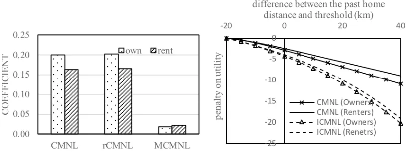
In terms of the penalty term in the models to simulate the choice set probability implicitly, our results show preferences consistent with the earlier statistical analysis (owners’ preference for alternatives close to the past home location is stronger than renters’ preference, Figure 1). The differences in the estimated values of the penalty term (µ) in ownership and renting models are found to be statistically significant (Figure 4a). Figure 4b also confirms that the penalty applied on owners’ utility due to the increase of distance of alternatives from their past home is always higher than that of renters. This means that alter-natives close to the current home have a higher probability to be included in the choice set of owners than renters. The direction of sensitivity (sign) of the explanatory parameters in the compensatory util-ity is found to be consistent both in the ownership and renting models but the sensitivutil-ity of several pa-rameters are found to be significantly different in both models (e.g., commute distance, distance from CBD, etc.).
[image:16.612.101.509.350.506.2](a) Estimated values of penalty parameters (b) Utility penalization
Figure 4. Impact of penalty terms on owners’ and renters’ choices
6
Validation results
Table 4. Final log-likelihood of models estimated for estimation subsets of owners data
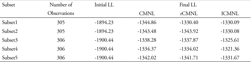
Table 5. Final log-likelihood of the models estimated for estimation subsets of renters data
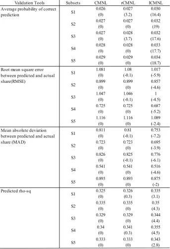
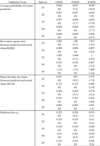
The five validation subsets (20% of the sample) are then used to validate the estimated model out-comes. The predictive power of each of the model is evaluated using both disaggregate level measures of fit (predictive rho-square and average probability of correct prediction) and aggregate level measures of fit (root mean square error and mean absolute deviation between predicted and actual share). Predictive measures of fit for all the models in different subsets are computed and summarized in Table 6 (owners subset) and Table 7 (renters subset) where the improvements in percentage over the CMNL model are presented in the parenthesis.
For owners, the ICMNL model shows improved performance over the CMNL and rCMNL mod-els in all subsets in terms of all measures of fit. However, the performance of the rCMNL model is same as the CMNL model performance in most of the subsets and marginally better in some cases in term of all measures of fit.
For renters, the ICMNL model performs better than the CMNL and the rCMNL models in all validation subsets in terms of the average probability of correct prediction and four out of five subsets (except subset 1) in terms of predicted rho-square. The ICMNL model performs worse than the CMNL and the rCMNL models in terms of root means square error and mean absolute deviation between actual and predicted share in one out of five subsets (subset S4). This is also likely due to the fact that this specific subset may contain a high concentration of observations where households have a lower preference for the alternatives close to their current homes.
Subset Number of
Observations Initial LL
Final LL
CMNL rCMNL ICMNL
Subset1 1500 -9315.90 -6173.75 -6173.42 -6048.39
Subset2 1500 -9315.90 -6207.40 -6207.11 -6091.69
Subset3 1500 -9315.90 -6195.84 -6195.24 -6079.12
Subset4 1500 -9315.90 -6224.88 -6224.35 -6107.48
Subset5 1500 -9315.90 -6183.15 -6182.45 -6065.08
Subset Number of
Observations
Initial LL Final LL
CMNL rCMNL ICMNL
Subset1 305 -1894.23 -1344.86 -1330.40 -1330.09
Subset2 305 -1894.23 -1343.48 -1343.92 -1330.08
Subset3 306 -1900.44 -1338.28 -1337.87 -1325.61
Subset4 306 -1900.44 -1334.37 -1334.02 -1321.36
[image:17.612.100.515.225.327.2]7
Conclusions
This study proposes an improvement of the existing CMNL model (called ICMNL model) for be-havioural choice set consideration with a better approximation to the classical Manski method. The proposed ICMNL model is evaluated in this study using simulated data and then applied to real-world residential location choice data. In both cases, better performance of the ICMNL model is observed compared to the existing CMNL and rCMNL model. Modelling of residential location choice with implicit choice set consideration also produces a behavioural difference in the choice set consideration of owners and renters.
Although the ICMNL model is found to outperform the CMNL and rCMNL models, it still has avenues for further improvements. The threshold effect considered in the model for utility penaliza-tion is exogenous and homogeneous across all respondents. The method can be improved by allowing individual specific threshold or threshold specific to the group of respondents belonging the same char-acteristics.
Further, the choice sets of all individuals in the proposed ICMNL model are constrained because utilities are penalized if alternatives do not meet the criteria of exogenous constraint. However, some individuals can have unconstrained choice sets in reality. Adopting latent classes in the ICMNL model could be a potential direction for further improvement of the proposed ICMNL model where the choice set of one class can be constrained and another class can be unconstrained. Considering the same attributes in the choice set part (in the penalty term) and in the systematic utility may result in an identification issue. The ICMNL model with latent classes for constrained and unconstrained choices set can avoid this issue. However, this technique cannot be applied in this study due to data limitation and could be a future direction of research.
Although the potential of the proposed method observed in this study to capture individual choice set is promising, more testing is recommended with other data sets as a topic of future research. Testing the validity of the findings in other contexts (e.g., route choice, destination choice, activity choice etc.) can also be an interesting direction for future research.
However, with better behavioural grounding (supported by the better model fit) as well as compu-tational tractability, the proposed ICMNL model can be an attractive option for modelling with a large universal choice set where the classical probabilistic approach is infeasible.
Acknowledgements
References
Arentze, T., & Timmermans, H. (2005). An analysis of context and constraints-dependent shopping behavior using qualitative decision principles. Urban Studies, 42(3), 435–448.
Bell, M. G. (2007). Mixed routing strategies for hazardous materials: Decision-making under complete uncertainty. International Journal of Sustainable Transportation, 1(2), 133–142.
Ben-Akiva, M., & Lerman, S. (1974). Some estimation results of a simultaneous model of auto owner-ship and mode choice to work. Transportation, 3, 357–376.
Bhat, C. R. (2015). A comprehensive dwelling unit choice model accommodating psychological con-structs within a search strategy for consideration set formation. Transportation Research Part B: Meth-odological, 79, 161–188.
Bhat, C. R., & Guo, J. (2004). A mixed spatially correlated logit model: Formulation and application to residential choice modelling. Transportation Research Part B: Methodological, 38(2), 147–168. Bhat, C. R., & Guo, J. Y. (2007). A comprehensive analysis of built environment characteristics on
household residential choice and auto ownership levels. Transportation Research Part B: Methodologi-cal, 41(5), 506–526.
Bierlaire, M., Hurtubia, R., & Flötteröd, G. (2010). Analysis of implicit choice set generation using a constrained multinomial logit model. Transportation Research Record: Journal of the Transportation Research Board, 2175, 92–97.
Caicedo, F., Lopez-Ospina, H., & Pablo-Malagrida, R. (2016). Environmental repercussions of park-ing demand management strategies uspark-ing a constrained logit model. Transportation Research Part D: Transport and Environment, 48, 125–140.
Cascetta, E., & Papola, A. (2001). Random utility models with implicit availability/perception of choice alternatives for the simulation of travel demand. Transportation Research Part C: Emerging Technolo-gies, 9(4), 249–263.
Cascetta, E., & Papola, A. (2009). Dominance among alternatives in random utility models. Transporta-tion Research Part A: Policy and Practice, 43(2), 170–179.
Castro, M., Martínez, F., & Munizaga, M. A. (2013). Estimation of a constrained multinomial logit model. Transportation, 40(3), 563–581.
Farooq, B., & Miller, E. J. (2012). Towards integrated land use and transportation: A dynamic disequi-librium-based microsimulation framework for built space markets. Transportation Research Part A: Policy and Practice, 46(7), 1030–1053.
Guevara, C. A. (2010). Endogeneity and sampling of alternatives in spatial choice models. (Unpublished doctoral dissertation) Department of Civil and Environmental Engineering, Massachusetts Institute of Technology, Cambridge, MA.
Habib, M., & Miller, E. (2009). Reference-dependent residential location choice model within a re-location context. Transportation Research Record: Journal of the Transportation Research Board, 2133, 92–99.
Haque, M. B., Choudhury, C., & Hess, S. (2018). Investigating the temporal dynamics of long-term and medium-term residential location choices: A case-study of London. Presented at the Transportation Re-search Board Annual Meeting, Washington, DC.
Kaplan, S., Bekhor, S., & Shiftan, Y. (2011). Development and estimation of a semi-compensatory residential choice model based on explicit choice protocols. The Annals of Regional Science, 47(1), 51–80.
Lee, B. H., & Waddell, P. (2010). Residential mobility and location choice: A nested logit model with sampling of alternatives. Transportation, 37(4), 587–601.
Manski, C. F. (1977). The structure of random utility models. Theory and Decision, 8(3), 22–254. Martínez, F., Aguila, F., & Hurtubia, R. (2009). The constrained multinomial logit: A
semi-compensa-tory choice model. Transportation Research Part B: Methodological, 43(3), 365–377.
Martínez, F., & Hurtubia, R. (2006). Dynamic model for the simulation of equilibrium status in the land use market. Networks and Spatial Economics, 6(1), 55–73.
Mcfadden, D. (1978). Modelling the choice of residential location. Transportation Research Record, 673, 72–77.
Næss, P. (2009). Residential self‐selection and appropriate control variables in land use: Travel studies. Transport Reviews, 29(3), 293–324.
Paleti, R. (2015). Implicit choice set generation in discrete choice models: Application to household auto ownership decisions. Transportation Research Part B: Methodological, 80, 132–149.
Rashidi, T. H., Auld, J., & Mohammadian, A. (2012). A behavioral housing search model: Two-stage hazard-based and multinomial logit approach to choice-set formation and location selection. Trans-portation Research Part A: Policy and Practice, 46(7), 1097–1107.
Scott, D. M. (2006). Constrained destination choice set generation: Comparison of GIS-based approaches. Presented at the Transportation Research Board 85th Annual Meeting, Washington, DC.
Swait, J. (2001). A non-compensatory choice model incorporating attribute cutoffs. Transportation Re-search Part B: Methodological, 35(10), 903–928.
Swait, J., & Ben-Akiva, M. (1987). Incorporating random constraints in discrete models of choice set generation. Transportation Research Part B: Methodological, 21(2), 91–102.
Termansen, M., McClean, C., & Skov-Petersen, H. (2004). Recreational site choice modelling using high-resolution spatial data. Environment and Planning B: Planning and Design, 36, 1085–1099. Zolfaghari, A. (2013). Methodological and empirical challenges in modelling residential location choices