Observing substructure in circumstellar discs around massive young stellar objects

young stellar objects

.

White Rose Research Online URL for this paper:

http://eprints.whiterose.ac.uk/137953/

Version: Accepted Version

Article:

Jankovic, MR, Haworth, TJ, Ilee, JD et al. (6 more authors) (2019) Observing substructure

in circumstellar discs around massive young stellar objects. Monthly Notices of the Royal

Astronomical Society, 482 (4). sty3038. pp. 4673-4686. ISSN 0035-8711

https://doi.org/10.1093/mnras/sty3038

© 2018 The Author(s) Published by Oxford University Press on behalf of the Royal

Astronomical Society. This is an author produced version of a paper published in Monthly

Notices of the Royal Astronomical Society. Uploaded in accordance with the publisher's

self-archiving policy.

[email protected]

https://eprints.whiterose.ac.uk/

Reuse

Items deposited in White Rose Research Online are protected by copyright, with all rights reserved unless

indicated otherwise. They may be downloaded and/or printed for private study, or other acts as permitted by

national copyright laws. The publisher or other rights holders may allow further reproduction and re-use of

the full text version. This is indicated by the licence information on the White Rose Research Online record

for the item.

Takedown

If you consider content in White Rose Research Online to be in breach of UK law, please notify us by

On Kelvin–Helmholtz and parametric instabilities driven

by coronal waves

Andrew Hillier

1

⋆

, Adrian Barker

2

, I˜

nigo Arregui

3

,

4

, Henrik Latter

5

1_{Department of Mathematics, CEMPS, University of Exeter, Exeter, EX4 4QF U.K.}

2_{Department of Applied Mathematics, School of Mathematics, University of Leeds, Leeds, LS2 9JT, U.K.} 3_{Instituto de Astrof´ısica de Canarias, V´ıa L´actea s/n, E-38205 La Laguna, Tenerife, Spain}

4_{Departamento de Astrof´ısica, Universidad de La Laguna, E-38206 La Laguna, Tenerife, Spain}

5_{Department of Applied Mathematics and Theoretical Physics, University of Cambridge, Wiberforce Road, CB3 0WA U.K.}

Accepted XXX. Received YYY; in original form ZZZ

ABSTRACT

The Kelvin–Helmholtz instability has been proposed as a mechanism to extract energy from mag-netohydrodynamic (MHD) kink waves in flux tubes, and to drive dissipation of this wave energy through turbulence. It is therefore a potentially important process in heating the solar corona. How-ever, it is unclear how the instability is influenced by the oscillatory shear flow associated with an MHD wave. We investigate the linear stability of a discontinuous oscillatory shear flow in the pres-ence of a horizontal magnetic field within a Cartesian framework that captures the essential features of MHD oscillations in flux tubes. We derive a Mathieu equation for the Lagrangian displacement of the interface and analyse its properties, identifying two different instabilities: a Kelvin–Helmholtz in-stability and a parametric inin-stability involving resonance between the oscillatory shear flow and two surface Alfv´en waves. The latter occurs when the system is Kelvin–Helmholtz stable, thus favouring modes that vary along the flux tube, and as a consequence provides an important and additional mechanism to extract energy. When applied to flows with the characteristic properties of kink waves in the solar corona, both instabilities can grow, with the parametric instability capable of gener-ating smaller scale disturbances along the magnetic field than possible via the Kelvin–Helmholtz

instability. The characteristic time-scale for these instabilities is∼100s, for wavelengths of200km.

The parametric instability is more likely to occur for smaller density contrasts and larger velocity shears, making its development more likely on coronal loops than on prominence threads.

Key words: instabilities — waves — Sun: corona – Sun: filaments, prominences —

Sun: magnetic fields

1 INTRODUCTION

Recent observations of oscillating prominence threads by the Interface Region Imaging Spectrometer (IRIS; De Pontieu et al. 2014) and the Hinode Solar Optical Tele-scope (Tsuneta et al. 2008) show that they can ‘fade out’

in cool lines (Caiiand Mgii) whilst simultaneously

emerg-ing in hotter lines (Siiv) (Okamoto et al. 2015). This could

be a signature of heating in these structures.Okamoto et al.

(2015) compared their oscillations in the plane-of-sky motion

(measured from Caiibroadband images) and in the

line-of-sight velocity field (from Dopplershifts in the Mgii K line

using spectra from IRIS); they found relative phase shifts of

these oscillations between90 degand180 deg. Forward

mod-elling of simulated data showed that these observed relative phase shifts are consistent with the resonant absorption of

⋆

E-mail: [email protected] (AH)

a magnetohydrodynamic (MHD) kink wave (Antolin et al. 2015).

A key component of the model ofAntolin et al.(2015)

is that the surface of an oscillating flux-tube can become un-stable to the Kelvin–Helmholtz (KH) instability (first seen associated with transverse kink waves in the simulations of Terradas et al. 2008), a shear-flow instability common in astrophysical systems. Instances of the occurrence of this instability include: the interaction of the solar wind with

the flanks of the magnetosphere (e.g.Hasegawa et al. 2004),

erupting regions (Ofman & Thompson 2011), the flanks

of coronal mass ejections (Foullon et al. 2011; M¨ostl et al.

2013), and where emerging magnetic flux interacts with

prominences (e.g. Berger et al. 2010; Ryutova et al. 2010;

Berger et al. 2017). The KH instability can drive turbu-lence and is a potential way to dissipate the energy of sur-face Alfv´en waves in magnetic flux tubes (Hollweg & Yang

1988;Ofman et al. 1994;Terradas et al. 2008;Antolin et al.

D

o

w

n

lo

a

d

e

d

fro

m

h

ttp

s:

//a

ca

d

e

mi

c.

o

u

p

.co

m/

mn

ra

s/

a

d

va

n

ce

-a

rt

icl

e

-a

b

st

ra

ct

/d

o

i/1

0

.1

0

9

3

/mn

ra

s/

st

y2

7

4

2

/5

1

2

4

4

0

0

b

y

U

n

ive

rsi

ty

o

f L

e

e

d

s

-

L

ib

ra

ry

u

se

r

o

n

2

6

O

ct

o

b

e

r

2

0

1

2015). So the key question is: How do these shear flows de-velop at the surface of an oscillating flux tube?

The existence of an unstable shear flow at the surface of a flux tube undergoing a transverse kink wave can be understood from the eigenfunction of the linear wave (e.g.

Sakurai et al. 1991;Goossens et al. 1992,2009). In the case

where the density is discontinuous at the surface of the tube, a discontinuous shear flow exists there, but this becomes

smooth for a continuous density profile (e.g.Goossens et al.

2009). However, for the smooth profile this shear flow can be enhanced by a process known as resonant absorption. First

proposed byIonson(1978), resonant absorption occurs

be-cause of a resonance between a kink wave travelling along a flux tube and an Alfv´en wave, which leads to a velocity singularity at the tube surface in ideal MHD (Sakurai et al.

1991;Goossens et al. 1992), though non-ideal effects make

this shear-flow velocity finite but large (Goossens et al. 1995). These small-scale flows enhance the dissipative

pro-cesses (Hollweg 1978;Wentzel 1974,1978,1979). Recent

the-oretical and numerical work has been devoted to transverse kink waves (Goossens et al. 2009), and has shown that their non-linear dynamics develop Kelvin–Helmholtz (KH)

unsta-ble flows (Terradas et al. 2008; Antolin et al. 2014, 2015,

2016,2017;Terradas et al. 2018). The instability acts to

ex-tract energy from the large-scale mode and to distribute it to smaller scales where dissipation can act effectively. The cause and nature of this eventual heating, however, is still under investigation (Magyar & Van Doorsselaere 2016;

Howson et al. 2017; Karampelas et al. 2017; Antolin et al.

2018). For a recent review of wave-based heating in the

so-lar atmosphere seeArregui(2015).

The general mechanism of the KH instability is that it breaks up the shear layer at the boundary between two flows by creating vortices (Chandrasekhar 1961). This may lead to turbulence via secondary 3D instabilities. For magneto-hydrodynamic flows, magnetic tension works to suppress the KH instability and favours unstable modes that do not vary along the field. To understand the growth of the magnetic

KH instability in coronal loops,Soler et al.(2010a)

investi-gated how it develops on the surface of a rotating flux tube. They found that the physics of the linear instability are not greatly altered by the change in geometry. However, the in-fluence of oscillations in the shear (as occurs in an MHD wave) on the growth of the instability is yet to be under-stood.

Oscillatory shear flows have been well studied in

hydro-dynamics. Kelley (1965) investigated the instability of an

oscillating shear flow including gravity and surface tension as suppression mechanisms for the classical KH instability. In the limit of zero-net shear flow (flow oscillating around a mean of zero), the instability can be described by a Math-ieu equation for the vertical displacement of the interface. This exhibits both a KH instability and a subharmonic para-metric instability driven by a resonance between the surface gravity waves and the oscillating shear flow, for different parameters.

Parametric instabilities occur in many circumstances when there is periodic forcing in a system that supports waves. If the wave has small amplitude, this instability is caused by the triadic interaction of the primary wave with a pair of (typically) smaller-scale daughter waves. For exam-ple, internal gravity waves in density stratified fluids, such as

the Earth’s oceans, are unstable to parametric instabilities that can transfer energy to smaller scales which are then

dis-sipated (McEwan & Robinson 1975;Drazin 1977). Another

example is that of rotating fluids with elliptical streamlines, which can be unstable to the elliptical instability, a para-metric instability involving the coupling of pairs of inertial waves with the elliptical deformation (Kerswell 2002). Of most relevance to this paper is the parametric instability of Alfv´en waves. This instability is believed to play a role in re-ducing the correlation between velocity and magnetic field fluctuations in the solar wind as the waves propagate out

into the heliosphere (e.g.Malara et al. 1996). The decay of

an Alfv´en wave via this instability has also been observed in experiments (Dorfman & Carter 2016).

An important extension to the work ofKelley (1965)

was performed by Roberts (1973). This work investigated

the development of the parametric instability in an oscil-lating MHD flow where the flow direction is aligned with the magnetic field. The magnetic field provides a tension that acts in a similar fashion to the surface tension treated

in Kelley (1965), working to suppress the KH

instabil-ity and enabling the existence of surface Alfv´en waves. If these waves are resonant with the oscillation frequency of the shear flow, they become parametrically unstable.

Zaqarashvili & Roberts (2002) extended this concept to

show that the parametric instability can drive the trans-fer of energy from fast magnetoacoustic waves into Alfv´en waves. One possible application of the MHD parametric in-stability has been the investigation of periodic gravitational forcing resulting in a field-aligned flow. Parametric growth of oscillations was found to result in an enhanced strength of a magnetic field through the parametric instability, with

application to the solar dynamo (Zaqarashvili 2000, 2001;

Zaqarashvili et al. 2002).

In this paper we investigate how the presence of an oscil-latory shear flow in the presence of a uniform magnetic field

perpendicular to the flow (i.e. the vorticity vector and the

magnetic field vector are aligned) can influence the develop-ment of the KH instability, or alternatively lead to paramet-ric instabilities. We analyse the simplest model possible: a discontinuous oscillatory shear flow in a local Cartesian do-main, and we derive the linear stability criteria analytically. We find that the oscillatory shear flow can be unstable to either the KH instability, or to a parametric instability in-volving the excitation of surface Alfv´en waves, depending on the parameters. Finally, we discuss the implications of our results for driving turbulence in the solar corona by kink waves.

2 MODEL AND LINEAR STABILITY

ANALYSIS

2.1 Model

Our motivation is to describe the development of the KH in-stability as this grows when driven by MHD oscillations in coronal flux tubes (an example of such a situation is shown

in Panel (a) of Fig.1). There are a number of possible flow

profiles associated with oscillations of a flux tube, two are

shown in the cross-sections shown in Panel (b) of Fig. 1.

However, this is a complicated configuration which would

D

o

w

n

lo

a

d

e

d

fro

m

h

ttp

s:

//a

ca

d

e

mi

c.

o

u

p

.co

m/

mn

ra

s/

a

d

va

n

ce

-a

rt

icl

e

-a

b

st

ra

ct

/d

o

i/1

0

.1

0

9

3

/mn

ra

s/

st

y2

7

4

2

/5

1

2

4

4

0

0

b

y

U

n

ive

rsi

ty

o

f L

e

e

d

s

-

L

ib

ra

ry

u

se

r

o

n

2

6

O

ct

o

b

e

r

2

0

1

[image:4.595.84.511.88.438.2]

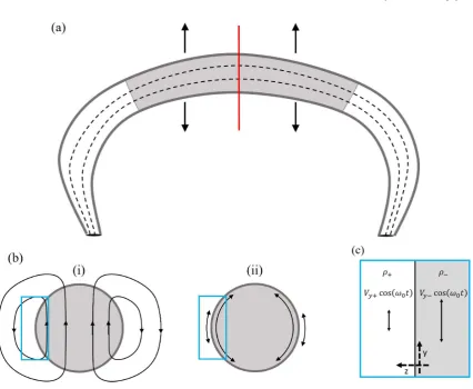
Figure 1.Panel (a): a large scale schematic diagram of an oscillating flux tube rooted in the solar photosphere. The black dashed lines show the magnetic field lines and the black arrows show the direction of oscillation. The shaded region represents dense material in the tube. The red line marks the position of the cross-section displayed in panel (b). Panel (b): image of the cross-section of the flux tube with flow patterns. The lines and arrows show: (i) a snapshot in time of the streamlines of the dipole flow formed around a kink-oscillating flux-tube (instability in this setting was investigated numerically by Terradas et al. 2008), note that the direction of the flow arrows will reverse periodically with the wave motion, and (ii) the shear-flow in a flux tube associated with surface Alfv´en waves (instability in this setting was investigated numerically byAntolin et al. 2015). The blue boxes show the local region modelled in this paper as shown in panel (c). Panel (c): diagram of the local Cartesian model investigated in this paper with different densities and magnitudes of the velocity field in the regions above and below the density jump. Both regions have a velocity field that oscillates in phase at the same frequency and have the same magnetic field strength, both in thex-direction.

be difficult to treat analytically. In this paper, we investi-gate a simpler problem that provides a good approximation to the relevant dynamics of this system. We perform a local Cartesian analysis looking at the apex of the flux tube, where the amplitude of the velocity shear driven by the fundamen-tal kink mode is largest, and the side of the flux tube with strong oscillatory shear flow with a setup shown in Fig. (1) panel (c). Thus in this model we have an oscillatory shear flow in the presence of a uniform horizontal magnetic field. Note that we neglect variations of the flow around and along the tube to allow us to make analytical progress. We also ne-glect the spatial and temporal variation of the magnetic field that would be associated with the magnetic oscillation. This is justified because the background flux tube is dominated by the axial component of the magnetic field.

The next approximation we make is that the oscillations in our model are driven by a periodic force in the momen-tum equation, not self-consistently via an MHD wave. As a result of our forcing there should be a pressure response in

the system, which we neglect because our focus is on incom-pressible disturbances (where the pressure response is small compared to the background pressure). This omission, how-ever, could be problematic when considering velocities com-parable with the fast-mode wave speed. We also neglect the magnetic field oscillations associated with the wave, as they are small in comparison to the background field along the flux tube, which should dominate the dynamics.

The equations governing our model are

∂ ρ

∂t +V· ∇ρ=0, (1)

ρ∂V

∂t +ρV· ∇V=− ∇P+J×B+F(z,t)ˆy, (2)

∂B

∂t =∇ ×(V×B), (3)

∇ ·V=0, (4)

∇ ·B=0, (5)

whereVis the velocity field,B is the magnetic field, ρthe

D

o

w

n

lo

a

d

e

d

fro

m

h

ttp

s:

//a

ca

d

e

mi

c.

o

u

p

.co

m/

mn

ra

s/

a

d

va

n

ce

-a

rt

icl

e

-a

b

st

ra

ct

/d

o

i/1

0

.1

0

9

3

/mn

ra

s/

st

y2

7

4

2

/5

1

2

4

4

0

0

b

y

U

n

ive

rsi

ty

o

f L

e

e

d

s

-

L

ib

ra

ry

u

se

r

o

n

2

6

O

ct

o

b

e

r

2

0

1

density,Pthe gas pressure,Jthe current density, andF(z,t)ˆy

is a forcing term that maintains an oscillatory shear flow of

frequencyω₀. We consider a shear flow in Cartesian

geome-try with the flow in they-direction, gradients in the flow in

the z-direction, and the magnetic field in thex-direction.

We take a uniform density in each layer, with the den-sity discontinuity aligned with that of the velocity, i.e. at

z=0. This is necessary for our basic oscillatory state to be

an exact solution of the governing equations. This state is described as follows:

ρ₀₌_



ρ₋ if z<0;

ρ₊ if z>0 , (6)

Vy,0=_



V₋cos(ω0t) ifz<0;

V₊cos(ω₀t) ifz>0 , (7)

Vx,0=Vz,0=0, (8)

P=P0, (9)

Bx,0=B, (10)

By,0=Bz,0=0. (11)

We also define the velocity difference∆V0=V₊−V₋. Here we

note that they-component of the background state equation

resulting from Eq. (2) is:

ρ0

∂Vy,0

∂t =F(z,t). (12)

The other equations are trivially satisfied by the background state.

2.2 Linear Analysis

Linearising about the basic state of an oscillatory shear flow

in the form G = G0+g, where G0 is a background state

variable andgis the corresponding linear perturbation, leads

to the following set of equations:

∂ ρ ∂t +Vy,0

∂ ρ ∂y +vz

∂ ρ₀

∂z =0, (13)

ρ0

∂v

∂t +ρ0Vy,0

∂v

∂y =− ∇p+j×B0, (14)

∂b

∂t =−Vy,0

∂b

∂y+ B∂v

∂x, (15)

∇ ·v₌0, (16)

∇ ·b₌0. (17)

Taking perturbations to be normal modes of the form

f(x,y,z,t)= f˜(z,t) exp(ikxx+ikyy) for the scalar quantities

andf(x,y,z,t)=˜f(z,t) exp(ikxx+ikyy) for vector quantities,

we may derive an equation for the temporal evolution of the

vertical Lagrangian displacement of the fluid (η˜z) which

re-lates to the z-component of the velocityv˜z=∂η˜z/∂t. Using

that the physical variables are constant in the regions both above and below the discontinuity and the requirement that

the perturbation decays to0at z=±∞in ideal MHD gives

the zdependence of the eigenfunction asexp(₋k_|z_|).

There-fore we can defineη˜z(z,t)=η(t) exp(−k|z|), and by matching

the solutions across the interface, the following equation for

ηis found:

d2η

dt2+2iky(α+V++α−V−)

dη

dt + "

iky α+ dV₊

dt +α− dV₋

dt !

(18)

−k2_y(α₊V₊2₊α₋V₋2)₊ k 2 xB2

2π(ρ₊₊ρ₋)

  η=0,

whereα_±=ρ_±/(ρ₊₊ρ₋). The derivation of this equation is

presented in AppendixA. If we setη=ηˆexp(−iky

R

α₊V₊+

α₋V₋dt), upon rearranging we get:

d2ηˆ dt2 +

  

k2xB2

2π(ρ₊₊ρ₋) −

1

2k

2

yα+α−∆V02(1+cos(2ω0t))

ηˆ=0. (19)

Using the Alfv´en speed in the ₊ region, i.e. V_{A+ =}

p B2_{/4π ρ}

+, and the wavenumber k0 we can determine the

following dimensionless quantities:

t= T

V_A+k₀, (20)

∆V ₌V_A+M_A, (21)

kx=k0Kx, (22)

ky=k0Ky, (23)

ˆ

η₌η′

k0

, (24)

whereT,∆V, Kx, Ky, andη′ are dimensionless and MA =

∆V/VA+is the Alfv´enic Mach number. For cases whereω0,0

we are free to selectk0 such thatω0=1, giving the

dimen-sionless equation:

d2η′ dT2 +

α₊

2 f

4K_x2−α₋K_y2M_A2(1₊cos(2T))gη′_{=0. (25)}

This is a Mathieu equation, which takes the general form:

d2f

dT2 +(a−2εcos(2T))f =0, (26)

where a and ε are constants. Eq. (25) is equivalent to

Eq. (26) if f =η′_{, and:}

a₌2α₊K2_x−1

2α+α−K

2

yMA2, (27)

ε₌1

4α+α−K

2

yMA2. (28)

This realisation is useful because the properties of the

Math-ieu equation are well understood (e.g. Bender & Orszag

1978).

2.3 General solutions to the Mathieu Equation

To understand the linear instabilities of an oscillating shear flow, it is helpful to first consider the general Mathieu equa-tion (Eq. (26)), and its resulting instabilities. We can rewrite Eq. (26) as:

d2f

dT2 +a f =2εcos(2T)f =ε exp(2iT)+exp(−2iT)

f. (29)

The solutions to this equation must obey Floquet’s theorem,

i.e. f ₌C₁exp(iωT)φ(T)₊C₂exp(₋iωT)φ∗_{(T), whereφ(T)is}

a function that is periodic with the same periodicity as the

time-varying coefficients,C₁andC₂are arbitrary constants,

D

o

w

n

lo

a

d

e

d

fro

m

h

ttp

s:

//a

ca

d

e

mi

c.

o

u

p

.co

m/

mn

ra

s/

a

d

va

n

ce

-a

rt

icl

e

-a

b

st

ra

ct

/d

o

i/1

0

.1

0

9

3

/mn

ra

s/

st

y2

7

4

2

/5

1

2

4

4

0

0

b

y

U

n

ive

rsi

ty

o

f L

e

e

d

s

-

L

ib

ra

ry

u

se

r

o

n

2

6

O

ct

o

b

e

r

2

0

1

and ∗ denotes the complex conjugate. Here φ(T) is given

byφ(T)=Σ∞_p

=−∞Apexp(2ipT), wherepis an integer. Using

this solution to f, inductive solutions to Eq. (29) can be

determined: f

−(ω+2p)2+agAp =ε(Ap₋1+Ap+1). (30) This is an infinite system of equations for the coefficients

Ap for each p. One can determineω from the requirement

that this system has non-trivial solutions. These consist of tongues of instability centred on certain frequencies.

Analytic solutions to these equations can be obtained

in the limitε≪1from Eq. (30). Forp₌0, we must have:

ω2_≈a, (31)

which describes an oscillation withω_=±√a. Forp,_0this

implies that to have a non-zero coefficientAp, we must have:

a₌p2, (32)

i.e. there is a resonance between the excited wave and the oscillatory forcing, which is a parametric instability. More generally, it can be shown that instability occurs within

fin-gers of instability (fora>0) that are bounded by

a=p2±ε+O(ε2), (33)

and the maximum growth rate at the centre of the dominant

p=1resonance is

σ_≡Im[ω]₌ε

2+O(ε

2_{), (34)}

(see, for example,Bender & Orszag 1978).

3 EXPLORING THE NATURE OF THE

INSTABILITIES

Now that we have an ODE in the form of a Mathieu equa-tion, we can explore the consequences of having an oscilla-tory shear flow. To gain intuition, it is helpful to consider the

case of constant shear (i.e. settingω0 =0so that the term

cos 2ω0t =1in Eq. (19)). In this regime we select our

nor-malising wavenumberk0to be an arbitrary real wavenumber

greater than 0. In this case the dimensionless Mathieu equa-tion becomes:

d2η′ dT2 +α+

f

2Kx2−α−Ky2MA2

g

η′=0, (35)

which has constant coefficients and normal mode solutions

of the formη′_∝exp(_±iωT). This leads to:

ω2=α+

2K2x−α−Ky2MA2

, (36)

where the first term arises from magnetic tension and is sta-bilising, while the second comes from the shear and is desta-bilising. In this equation the first term on the RHS is the square of the MHD kink wave frequency in the incompress-ible limit, which describes a surface Alfv´en wave, and the second term describes the Doppler-shifting of this wave by the shear flow. When the second term becomes larger than

the first,ω2 is negative and the system is unstable to the

MHD KH instability with a growth rate given by |ω| (e.g.

Chandrasekhar 1961). This can be mathematically stated as the following condition for the onset of instability:

M_A2 > 2K

2 x

α₋Ky2

. (37)

Simply put, if the Alfv´enic Mach number becomes suffi-ciently large, for a given wavevector direction, then the shear flow can overcome magnetic tension and the system becomes unstable. If there is no perturbation at all in the direction

of the magnetic field (Kx=0) then there is no suppression

by magnetic tension and the system is unstable forany

non-zero velocity difference. But as the angle of the wavevector to the magnetic field tends towards zero the driving force is reduced and the tension force is increased so the system

tends towards stability. TheKx=0modes are rather special

as they would correspond in our model to modes with no, or possibly global, variation along the flux tube; instead, their variation is confined primarily to around the circumference of the flux tube.

When the oscillatory term is included (i.e.ω0,0, and

we solve Equation25), then as inKelley (1965) andRoberts

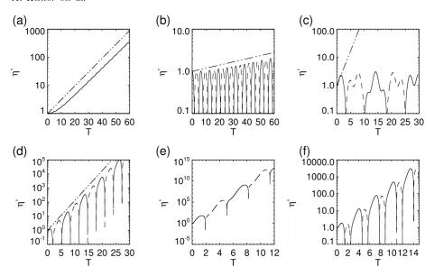
(1973) then both the KH instability and parametric insta-bilities will be possible. This can be seen in Fig. (2), which

gives numerical solutions to the temporal evolution of η′

from solving Eq. (25) first by splitting this equation into

two coupled equations forη′ _anddη′_{/dT and solving these}

with a first order, forward difference solver. Solutions are

given forM_A=0.2, andα₊₌0.01for different points inK

-space (these points inK-space are shown in Fig.3). These

show a KH unstable mode (panel a),p=1parametric

unsta-ble modes (panels b, d, e),p=2parametric unstable mode

(panel f), and a stable mode (panel c). Looking at this fig-ure, it is clear to see that the KHI is a direct instability of our system (shown by the fact there is only a solid black line in panel a), but the parametric instability involves a reso-nantly enhanced wave so the solution takes both positive and negative values (see the switch between solid - positive

η′ _{- and dashed - −η}′ _{- lines in panel b). We explore the}

different instability behaviour in this section.

3.1 Properties of the instabilities in the limit of

weak shear

In this section we consider a limit of Eq. (19) where the

am-plitude of the oscillatory shear flow (proportional tocos 2T)

is small in a similar fashion to Section2.3, as also considered

byKelley (1965) andRoberts(1973). We use this to develop

solutions for the growth rate of the two instabilities. Strictly

speaking, we takeε≪1(as defined in Eq. (28)) and follow

the method presented in Bender & Orszag (1978).

Physi-cally this corresponds to the limit where the square of the shear rate is small compared to the square of the oscillation frequency, and one example where this may occur is when the wave driving the shear flow has a small amplitude.

3.1.1 Magnetic KH instability

From Section2.3when the resonance condition is not

sat-isfied then the wave frequency is given byω_=±√a and by

direct comparison it is possible to state the frequency of the surface wave in the small shear limit. This is given as:

ω=±

r

α₊

2 q

4Kx2−α−Ky2M_A2. (38)

This is very similar to Equation36, the only difference being

that the second term underneath the square root is a factor

D

o

w

n

lo

a

d

e

d

fro

m

h

ttp

s:

//a

ca

d

e

mi

c.

o

u

p

.co

m/

mn

ra

s/

a

d

va

n

ce

-a

rt

icl

e

-a

b

st

ra

ct

/d

o

i/1

0

.1

0

9

3

/mn

ra

s/

st

y2

7

4

2

/5

1

2

4

4

0

0

b

y

U

n

ive

rsi

ty

o

f L

e

e

d

s

-

L

ib

ra

ry

u

se

r

o

n

2

6

O

ct

o

b

e

r

2

0

1

0 10 20 30 40 50 60

T

1

10

100

1000

η

’

0 10 20 30 40 50 60

T

0.1

1.0

10.0

η

’

0 5 10 15 20 25 30

T

0.1

1.0

10.0

100.0

η

’

(a)

(b)

(c)

0 5 10 15 20 25 30

T

10

-1

10

0

10

1

10

2

10

3

10

4

10

5

η

’

0 2 4 6 8 10 12

T

10

-5

10

0

10

5

10

10

10

15

η

’

0 2 4 6 8 101214

T

0.1

1.0

10.0

100.0

1000.0

10000.0

η

’

[image:7.595.53.525.85.391.2]

(d)

(e)

(f)

Figure 2.Calculation of the variation ofη′ _{withT forMA=0.2, andα}

+=0.01usingθ=1.48(whereθ=tan−1(Ky/Kx)) in panels (a) and (c),θ=1.20in panel (b),θ=1.45in panel (d),θ=1.5in panel (e), andθ=1.45in panel (f).K=20(whereK=

q Kx2+K

2

y) is used for panels (a) and (b),K=100for (c) and (d),K =300for (e) andK =200for (f). The dash-triple dot line in panels (a) to (d) gives

the predicted growth rate. The solid lines show positive and the dashed lines negative values ofη′_{. The positions inK-space for each of}

these panels are marked on Fig. (3).

of1/2smaller, that results from averaging the shear kinetic

energy over one period.

To have a direct instability of the system, the stiffness of the boundary between the two flows (i.e. the flux tube boundary) needs to disappear, i.e.:

M_A2 > 4K

2 x

α₋Ky2

, (39)

which means that the non-oscillatory term in Eq. (19) is neg-ative. For instability the Alfv´enic Mach number has to be

√

2greater than the case with the same wavevectorK for a

non-oscillatory shear flow (see Eq. (37)). As can be expected for the MHD KH instability, the shorter the wavelength in the direction of the flow and the longer the wavelength in the direction of the magnetic field the more likely the sys-tem is to be unstable. Though it is important to remember that for this inequality to accurately describe the onset of

direct instability, 1₄α+α−K2yM_A2 ≪ 1. Figure (2) panel (a)

compares the predicted growth rate of the KH instability to the solution of Eq. (25) showing that for these param-eters the solution in the asymptotic limit and the solution match well. For panel (c), though predicted to be unsta-ble in the asymptotic limit, the KH mode does not grow for these parameters as they are beyond the applicability of this

limit. We will look at this further in Section3.2. Note that

θ₌tan−1_(K y/Kx).

3.1.2 Subharmonic resonance

If the system is stable to the KH instability, then a perturba-tion takes the form of a surface wave instead. The frequency of the surface shear Alfv´en wave is given by Eq. (38). There exists a parametric resonance between this wave and the

os-cillatory driver when, as stated in Section2.3, the following

condition is satisfied:

ω2=a=p2, for p=1,2,3, ... (40)

Note this is different to the resonance process behind

res-onant absorption discussed in Section 1. As the strongest

resonance occurs forp₌1, then the fastest growing modes

satisfy:

ω=±1, (41)

which is equal to half the frequency of the oscillatory forc-ing, indicating subharmonic resonance. This corresponds to counter-propagating surface Alfv´en waves that become un-stable if their frequency magnitudes are equal to the fre-quency of the oscillatory shear flow.

The parametric instability is not just confined to the exact resonance, there is an envelope around this exact reso-nance that is unstable (see e.g. Section 2.3), with the width

of the envelope being given by 2ε (e.g. Bender & Orszag

1978). We note here that for a larger Alfv´enic Mach number

or α₊ ∼α₋ then more of the parameter space is unstable

to parametric instabilities because ε becomes larger. From

D

o

w

n

lo

a

d

e

d

fro

m

h

ttp

s:

//a

ca

d

e

mi

c.

o

u

p

.co

m/

mn

ra

s/

a

d

va

n

ce

-a

rt

icl

e

-a

b

st

ra

ct

/d

o

i/1

0

.1

0

9

3

/mn

ra

s/

st

y2

7

4

2

/5

1

2

4

4

0

0

b

y

U

n

ive

rsi

ty

o

f L

e

e

d

s

-

L

ib

ra

ry

u

se

r

o

n

2

6

O

ct

o

b

e

r

2

0

1

this we can define the following band where the dominant subharmonic parametric instability is possible:

3

8α−K

2

yMA2 >Kx2− 1

2α₊ >

1

8α−K

2

yMA2. (42)

The maximum growth rate of the instability happens when the exact resonance condition is satisfied. This growth

rate is given by (e.g.Bender & Orszag 1978):

σmax=ε

2 =

1

8α+α−K

2

yM_A2. (43)

Of note here is the dependence of the growth rate on M_A2.

This is contrary to the KH modes, which grow at a rate

pro-portional toMA. Figure (2) panels (b) and (d) compare the

predicted growth rate of the parametric instability to the so-lution of Eq. (25) with a first order forward difference solver for the same parameters with the solution in the asymptotic limit proving to be accurate.

From this analysis we can see that the parametric in-stability is quite different to the magnetic KH inin-stability.

While the latter grows fastest for modes that minimise Kx

(i.e. wavelengths along the magnetic field as long as possible are preferred), modes unstable to the parametric instability

must have finite Kx. Therefore it is the parametrically

un-stable modes that are good at kinking and disturbing the

boundary between the two flows along the direction of the

magnetic field.

3.2 Solutions to the Mathieu Equation

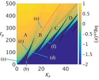
Figure (3) plots the base 10 logarithm of the growth rate

and shows the regions of instability on the (Kx,Ky)-plane.

The values were computed by solving Eq. (25). In this figure,

α₊ =0.01 and MA =0.2. We analyse Eq. (25) numerically

using a Floquet method. First, we write Eq. (25) as a system of 2 coupled ODEs. We then compute the monodromy ma-trix of linearly independent solutions, which is accomplished

by integrating the ODEs over one periodπfor initial

condi-tions such that all variables except one are set to zero (using a 4/5th order Runge–Kutta method). The eigenvalues of the monodromy matrix allow us to obtain the complex growth rates of the instability. As can be seen in Fig. (3) there are regions of stability (blue) but also bands of instability shown in green and yellow.

In Fig. (3) there are a number of bands inK-space where

the system becomes unstable. There are two distinct insta-bilities that exist in the unstable bands. In the band in the

top left (associated with smallKx), above the green dashed

line, the system is KH unstable (see panel (a) of Fig. (2)). However, the other bands are related to the resonant growth of waves (see panels (b) and (d) of Fig. (2)). Panel (c) shows a region that is expected to be KH unstable based on the asymptotic limit, but the instability is switched off as it is impinged by the resonance. The instability bands are well

separated for smallKy, but asKyincreases the resonance

im-pinges on the KH instability. In Fig.3the dashed green line

marks the theoretically predicted cutoff for the KH

instabil-ity (see Section3.1.1) and the solid red line with the dashed

red lines mark the p = 1 subharmonic resonance growing

through a parametric instability (see Section3.1.2). For the

parameters used in the calculation of Fig.3the asymptotic

limits are expected to hold whenKy≪100(i.e.ε≪1).

From Fig. (3) we can see that, though crude, where the upper bound of the parametric instability as calculated by the asymptotic limit meets the marginal stability curve of the KH instability (again in the asymptotic limit) can be used as an approximate wavevector for where the resonance begins to impinge on the KH instability. This wavevector is given by:

Kx=√1_α

+

, (44)

Ky=√ 2

α₊α₋

1 MA

. (45)

Figure3 shows a total of five parametrically unstable

regions, which are associated with p=1 to 5in Eq. (40).

Each of these fingers of instability start from Ky =0, i.e.

from the x-axis, but because as pgets larger the resonance

gets weaker the fingers of instability get thinner. This makes

them harder to accurately plot in the figure nearKy=0as

they are more challenging to resolve inK-space. For a given

Ky, we find that the largest growth rate is associated with

a KH mode, with thep=1resonance next largest, and the

growth rate getting smaller aspincreases.

In the region of the figure above the dashed green line, the asymptotic limits predict that this is unstable every-where, and this is generally correct. However, it is

impor-tant to note that even in this regime, where a, as defined

in Eq. (27), is negative, the regions of parametric

instabil-ity appear. Even witha <0these parametric unstable

re-gions still represent the exponential growth of an oscillation around zero and not a purely growing mode (as shown in Fig. (2) panel (e)). Compared to the non-oscillatory case,

the key change in stability of the system comes whena is

positive, i.e. below the dashed green line, and resonances can drive perturbations to the system to grow.

4 APPLICATION TO THE SOLAR

ATMOSPHERE

Now let us take the model back to its application to coro-nal flux tubes. When considering the instability on an os-cillating flux tube in the solar atmosphere, firstly the dif-ferent scales of the problem need to be considered. For a

prominence thread, the diameter (D) is often of the order

of 2×102km (e.g. Arregui et al. 2018) but can be up to

103km (e.g.Okamoto et al. 2015). The length (L, taken as

the distance of the field lines leaving the photosphere to their return) can be two or more orders of magnitude greater

thanD. The length of the flux tube filled with dense

mate-rial is often found to be between∼3×103 and 3×104km

(Arregui et al. 2018). If the wavenumber associated with the instability on the flux-tube surface is considered, then it must necessarily have a larger aspect ratio with the flux-tube length than the diameter. Roughly speaking these numbers hold for coronal loops (flux tubes that are filled with hot material) as well.

To use this aspect ratio to constrain our calculations, we need to determine a lower limit for the normalised

wavenum-berKgiven by the length of the flux tube in normalised form.

If a flux-tube is oscillating in the solar corona, the char-acteristic frequency of the oscillation is the kink frequency

D

o

w

n

lo

a

d

e

d

fro

m

h

ttp

s:

//a

ca

d

e

mi

c.

o

u

p

.co

m/

mn

ra

s/

a

d

va

n

ce

-a

rt

icl

e

-a

b

st

ra

ct

/d

o

i/1

0

.1

0

9

3

/mn

ra

s/

st

y2

7

4

2

/5

1

2

4

4

0

0

b

y

U

n

ive

rsi

ty

o

f L

e

e

d

s

-

L

ib

ra

ry

u

se

r

o

n

2

6

O

ct

o

b

e

r

2

0

1

[image:9.595.119.468.110.391.2]

Figure 3.Numerically computed logarithm of the growth rate inK-space. Blue regions are approximately stable (withσ≤10−2_{). The} top left region (which emanates fromKx =Ky =0) is KH unstable, whereas the five fingers of instability (yellowish regions pointing down) to the right of the KH band (associated withKx=p/

√₂

α+forKy =0) are parametrically unstable. These fingers of instability are associated withp=1to5in equation40. The capital letters A to D mark different instability bands, where A= KH instability, B= Parametric (p=1), C= Parametric (p=2), D= Parametric (p=3). The green dashed line marks the critical wavenumber for the growth of the KH instability in the asymptotic limit. The solid red line gives the fastest growing parametric mode in the asymptotic limit, with the dashed red lines marking the band of approximate resonance valid for small Ky. In this calculationα+=0.01and MA=0.2. The labelled blue arrows show the position inK-space of the six calculations shown in Figure2.

and the characteristic speed is the kink speed. As the

non-dimentional kink speed of a flux tube is√2α+, the frequency

of the surface Alfv´en wave will, because it is driven by res-onance with the kink-wave, equal the frequency of a global linear kink wave of the flux tube and have a normalised value

of unity. Therefore, theKxvalue (forKy=0) that gives this

isKx,KINK=1/√2α₊, which is theKx value associated with

the first resonance forKy=0. By takingKx≥Kx,KINKthen

we can look at wavenumbers that are appropriate for com-paring to instabilities in coronal flux tubes. For an aspect

ratio of the flux tube of1 : 100then instability modes must

haveKy≥Ky,D=1/D=200/√2α₊ whereDis the diameter

of the flux tube.

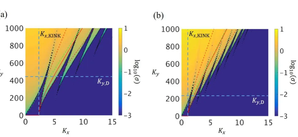
Figure (4) shows calculations with density ratios of 1:10

(panel a) and 2:3 (panel b), andMA=0.02, calculated using

a coronal Alfv´en speed of 1000km s−1 _{and a velocity}

dif-ference of 20km s−1_{. Generally the structure of the bands}

of instability is very similar to that shown in Fig. (3). Both

Kx,KINKandKy,Dare marked with dashed blue lines, and we

expect that instabilities on a flux tube will have to be in the quadrant that is to the right of the dashed blue line marked

Kx,KINK and above the dashed blue line markedKy,D.

If we only look at modes that useKx,KINK then for all

Ky there is no parametric instability only KH instability.

This instability provides the largest growth rate for a given

Ky, but for all Ky the growth rate is reduced compared to

Eq. (38) as a result of the presence of the resonance, i.e. for all achievable growth rates of the KH instability on a flux-tube, the oscillatory nature of the shear and the impinging parametric resonance band reduces the growth of the KH instability. These large scale modes are strictly outside the domain of applicability of the local model we have developed. To fully understand the dynamics of this global mode then the boundary conditions and variations along the flux tube would have to be included.

If we look at smaller scales along the flux tube, which is more consistent with the local model we employ, this would

mean that we should usenKx,KINKas the wavenumber along

the magnetic field wherenis a integer greater than1. This

puts the system into a regime where parametric instabilities

dominate at the smallest unstableK values (which, due to

the larger spatial scales involved, can extract more energy from the shear flow). Because these instabilities exist for different wave vectors, it can be expected that both of the instabilities could be growing in a system at the same time. For an instability, either KH or parametric, with

2Ky,D ≤ Ky ≤ 4Ky,D, from Fig. (4) the growth rate is in

the rangeσ _{= |}iω_{| ∼}1to 10_×ω₀. Taking a characteristic

oscillation period of a kink wave in the corona to be300s,

then the time scale for the instability is approximately30to

D

o

w

n

lo

a

d

e

d

fro

m

h

ttp

s:

//a

ca

d

e

mi

c.

o

u

p

.co

m/

mn

ra

s/

a

d

va

n

ce

-a

rt

icl

e

-a

b

st

ra

ct

/d

o

i/1

0

.1

0

9

3

/mn

ra

s/

st

y2

7

4

2

/5

1

2

4

4

0

0

b

y

U

n

ive

rsi

ty

o

f L

e

e

d

s

-

L

ib

ra

ry

u

se

r

o

n

2

6

O

ct

o

b

e

r

2

0

1

[image:10.595.53.540.92.315.2]

Figure 4. Numerically computed logarithm of the growth rate in K space for (a)α+=1/11and MA =0.02and (b) α+ =2/5and MA=0.02. In each panel the green dashed line marks the critical wavenumber for the growth of the KH instability in the asymptotic limit. The solid red line give the fastest growing parametric mode in the asymptotic limit, with the dashed red lines marking the band of approximate resonance. The vertical dashed blue lines show the position of Kx,KINK and the horizontal dashed blue lines show the position ofKy,D. The top right quadrant, which is most relevant for instability in a solar setting, is dominated by parametric modes.

300s. Note that these parametric modes are associated with

positions inK-space above the dashed green lines in Fig. (4).

For perturbations below that line (i.e. regions that would be stable for a non-oscillatory shear flow) the growth rate will

beσ≤ω0, and so these perturbations can grow (with high

wave number along the magnetic field) at time scales longer

than300s and as such can still occur on dynamically

impor-tant times scales. Prominence threads may have a density up

to100times greater than the solar corona (e.g.Parenti 2014;

Arregui et al. 2018), for this case the structure of the insta-bility bands would not change significantly and we would expect instability to grow on a time scale of approximately

30s, as estimated using Fig.3. As this time scale will connect

to the rotation time of a vortex at that scale (i.e. the eddy turnover time), this time scale can also be used as a lower estimate of the turbulence time scale (and with it the heat-ing time scale) of the flux tube, though nonlinear analysis is necessary to accurately estimate this value.

It is important to note here that for instability in a prominence thread, we have imagined a loop in the solar corona comprised of a flux tube that is completely filled by dense material, and used this to connect the length scales of the first resonance in the model to the loop length (or thread length as they are treated as being the same). How-ever, the reality is that only a section of the loop will contain

this material (e.g.Arregui et al. 2018).Soler et al. (2010b)

investigated the change in period of a kink-wave as a result of the prominence thread only filling part of the flux tube, finding that the frequency of the wave changes. The reduc-tion in the period of a fundamental kink mode by a factor of two if the dense thread only fills 10 per cent of the flux tube instead of the whole tube (Arregui et al. 2011). This change in frequency from the local kink frequency will mean

that the position of the resonance relative to Kx.KINK will

change, but as this is not a large change it would not be expected to greatly influence our estimates.

5 SUMMARY AND DISCUSSION

This paper demonstrates that an oscillating MHD shear flow is unstable to not only the KH instability, but also to para-metric instabilities involving surface Alfv´en waves. In gen-eral the growth rate of the KH instability is larger than

that of the parametric instability, but asε(which quantifies

the magnitude of the shear flow) becomes large the reso-nances can impinge on the KH instability, pushing the criti-cal wavenumber for direct instability to higher wavenumber

K. This is of importance for understanding the growth of the

KH instability at the surface of prominence threads or coro-nal loops because the oscillatory nature of the shear changes the onset of the KH instability.

The general characteristics of the instabilities found in the model are:

(i) The frequency of a surface Alfv´en wave in the limitε_≪1is

modified by the oscillating flow, which is given in Eq. (38). (ii) There exist surface Alfv´en waves that become resonant

with the oscillatory driver as a result of the Doppler-shifting of their frequencies by the flow. These waves undergo an exponential growth in amplitude. In the asymptotic limit of weak shear, the exponential growth associated with the

strongest resonance can be calculated and is given in Eq.43.:

(iii) Beyond this limit, the region inK-space where the

paramet-ric instability can grow approaches the KH unstable band, suppressing the KH instability in this region.

(iv) We expect that both these instabilities could exist in the

solar atmosphere with characteristic time scales of∼100s,

for wavelengths of200km around the flux tube.

D

o

w

n

lo

a

d

e

d

fro

m

h

ttp

s:

//a

ca

d

e

mi

c.

o

u

p

.co

m/

mn

ra

s/

a

d

va

n

ce

-a

rt

icl

e

-a

b

st

ra

ct

/d

o

i/1

0

.1

0

9

3

/mn

ra

s/

st

y2

7

4

2

/5

1

2

4

4

0

0

b

y

U

n

ive

rsi

ty

o

f L

e

e

d

s

-

L

ib

ra

ry

u

se

r

o

n

2

6

O

ct

o

b

e

r

2

0

1

Returning to our initial motivation, though we use a highly simplified model when applied to the disruption of oscillating structures in the solar atmosphere, there are a number of conclusions we can draw. For an oscillating mag-netic field in the solar atmosphere, the boundary conditions require modes to have wavenumbers along the magnetic field

of Kx>0. In fact, we calculate the minimumKx to be the

point at which the surface Alfv´en wave, unmodified by the shear, would resonate with the driving frequency. Due to the strengths of the magnetic field, most of the modes of inter-est would have to have the ratio of wavenumbers across and

along the magnetic field ofKy/Kx ≪1. One clear result of

this study is that the instabilities that can develop from an oscillating flow are more complex than the KH instability of a non-oscillatory shear flow. We can expect that resonances would play a role, and when the KH does grow, any vortices that are created will reverse the sign of their vorticity line with the change in sign of the vorticity of the forcing (in the solar case this is the large scale MHD wave).

The key point of this paper is that if we account for the oscillatory nature of a wave in a flux tube, then we find that there are two types of instabilities, and that they can be ex-cited for a wider range of wavenumbers (especially along the magnetic field) compared with the case of a constant shear. As such there are a richer array of disturbances on shorter scales along the magnetic field, and hence of ways to break down the original Alfv´enic wave, and possibly to disturb the underlying flux tube. An interesting extension to this work would be to perform a similar analysis on the surface of a

flux tube similar to the model of Soler et al. (2010a) but

considering an oscillating flow. Because the modes around the surface of a flux tube are quantised, as are the modes along a flux tube of finite length, this will make it harder to satisfy exact resonance, which could have an impact on the nature of the instability.

The existence of these two instabilities may have inter-esting consequences for the potential development of turbu-lence in the system under study. The non-linear development of the hydrodynamic KH instability can produce turbulence without a magnetic field. In the MHD limit, there are extra

complexities, but as shown in Antolin et al.(2015) chaotic

turbulent-like flows can develop. The existence of parametric instabilities also has a connection to MHD turbulence, since the instability involves wave-interactions, which are also

cru-cial for Alfv´enic turbulence (e.g.Goldreich & Sridhar 1995).

It has been shown that the saturation of the parametric in-stability can have quite rich dynamics, giving rise to non-linear oscillations, chaotic wave-wave interactions, and dis-ordered wave turbulence (Wersinger et al. 1980). Therefore, the two MHD instabilities that can be expected to develop as a result of the oscillating shear flow we have studied po-tentially connect to the development of two different regimes of turbulence in an MHD system.

The parametric instability can grow at larger scales across the magnetic field when the Alfv´enic Mach number

MAof the oscillating flow is increased or the density contrast

between the two flow regions is decreased. Dynamically this would be distinguished from a direct instability by the pro-gressive increase in amplitude of a wave instead of the linear growth of a perturbation. In the solar atmosphere, this den-sity contrast is smaller in coronal loops than in prominence threads, making the parametric instability more likely to

oc-cur for coronal loop oscillations. It is necessary to perform a range of MHD simulations to see if resonant enhancement of surface waves can happen at dynamically important scales under solar conditions. As the importance and the growth

of the instability scales asM2

A, this could result in changes

to the rate at which oscillations damp for increasing

nonlin-earity of the oscillation.Goddard & Nakariakov(2016)

ob-served such a trend in coronal loops and it would be inter-esting to develop this connection.

ACKNOWLEDGEMENTS

The authors would like to thank Prof. Andrew Gilbert for his comments which greatly improved the content of the manuscript. AH is supported by his STFC Ernest Ruther-ford Fellowship grant number ST/L00397X/2 and by STFC grant ST/R000891/1. AJB was supported by the Lever-hulme Trust through the award of an Early Career Fellow-ship and by STFC Grant ST/R00059X/1. IA acknowledges financial support from the Spanish Ministry of Economy and Competitiveness (MINECO) through projects 55456-P (Bayesian Analysis of the Solar Corona), AYA2014-60476-P (Solar Magnetometry in the Era of Large Tele-scopes), from FEDER funds, and through a Ramon y Cajal fellowship.

APPENDIX A: FULL LINEAR STABILITY ANALYSIS

Linearising about the basic state of an oscillatory shear flow,

we expand each variable in the formG₌G₀₊g, whereG0

is a basic state variable andgis its linear perturbation, we

obtain the following set of equations:

∂ ρ ∂t +Vy,0

∂ ρ ∂y+vz

∂ ρ₀

∂z =0, (A1)

ρ0

∂v

∂t +ρ0Vy,0

∂v

∂y +ρ0vz

∂Vy,0

∂z ˆj=− ∇p+j×B0, (A2)

∂b

∂t +Vy,0

∂b

∂y =− bz

∂Vy,0

∂z ˆj+B

∂v

∂x, (A3)

∇ ·v₌0, (A4)

∇ ·b₌0, (A5)

whereˆjis the unit vector in the y direction. We assume

nor-mal modes of the form f(x,y,z,t) = f˜(z,t)ex p(ikxx+ikyy),

D

o

w

n

lo

a

d

e

d

fro

m

h

ttp

s:

//a

ca

d

e

mi

c.

o

u

p

.co

m/

mn

ra

s/

a

d

va

n

ce

-a

rt

icl

e

-a

b

st

ra

ct

/d

o

i/1

0

.1

0

9

3

/mn

ra

s/

st

y2

7

4

2

/5

1

2

4

4

0

0

b

y

U

n

ive

rsi

ty

o

f L

e

e

d

s

-

L

ib

ra

ry

u

se

r

o

n

2

6

O

ct

o

b

e

r

2

0

1

and obtain the following system of linear equations:

Dρ₊v˜z

∂ ρ0

∂z =0, (A6)

ρ0Dv˜x=−ikxp˜, (A7)

ρ0Dv˜y+ρ0v˜z

∂Vy,0

∂z =−ikyp˜+ B

4π(ikxb˜y−ikyb˜x), (A8)

ρ0Dv˜z=−∂p˜

∂z − B

4π

∂b˜x

∂z −ikxb˜z !

, (A9)

Db˜x=ikxBv˜x, (A10)

Db˜y+bz

∂Vy,0

∂z =ikxBv˜y, (A11)

Db˜z=ikxBv˜z, (A12)

ikxv˜x+ikyv˜y=−∂v˜z

∂z , (A13)

ikxb˜x+ikyb˜y=−∂ ˜ bz

∂z , , (A14)

where D=∂/∂t+ikyVy,0, i.e. the advective derivative.

The first step is to take thexderivative of Eq. (A7) and

add this to they-derivative of Eq. (A8) and in conjunction

with Eqs. (A13) and (A14) gives:

−ρ₀D∂v˜z

∂z +ρ0v˜z

∂Vy,0

∂z =k

2_p˜−ikxB

4π

∂b˜z

∂z + k2B

4π b˜x. (A15)

From here we can introduce the Lagrangian displacementη˜

defined by

˜

vx=Dη˜x, (A16)

˜

vz=Dη˜z, (A17)

which implies that

˜

bx=ikxBη˜x, (A18)

˜

bz=ik x Bη˜z. (A19)

Substituting these into Eqs. (A9) and (A15) leads to:

−ρ0D2

∂η˜z

∂z =k

2_p˜ +k

2

xB

4π

∂η˜z

∂z +ikx k2B2

4π η˜x, (A20)

ρ0D2η˜z=−∂p˜

∂z −ikx B2

4π

∂η˜x

∂z −ikxη˜z !

. (A21)

It is simple to show that:

−∂p˜

∂z = 1 k2

∂ ∂z

 k2xB

4π

∂η˜z

∂z +ikx k2B2

4π η˜x+ρ0D

2∂η˜z

∂z 

, (A22)

which substituted into Eq. (A21) gives:

∂ ∂z

  

ρ0D2+k 2

xB

4π

  ∂∂η˜zz

 −k2



ρ0D2+k 2 xB2

4π



η˜z =0. (A23)

Looking at Eq. (A23) atz,_0gives:



ρ₀D2+k 2

xB

4π



 _∂∂_z22 −k 2

! ˜

ηz=0. (A24)

We know that at thez-dependence of the solution is of the

form exp(−k|z|), which is the same as in the MHD KH

in-stability with constant shear (Chandrasekhar 1961). Using

the continuity ofη˜z at the boundary, we have that:

˜

ηz(z,t)=η(t) exp(−k|z|). (A25)

Equation (A23) can be integrated over the discontinuity to give:

 ρ0D2++

k2_xB

4π

 η+



ρ0D2₋+k 2

xB

4π



η=0, (A26)

or, in full,

d2η

dt2 +2iky(α+V++α−V−)

dη

dt + "

iky α+ dV₊

dt +α− dV₋

dt !

−k2y(α+V+2+α−V−2)+

k2xB2

2π(ρ₊₊ρ₋)

 

η=0, (A27)

whereα_±=ρ_±/(ρ++ρ−).

If we define η =ηˆexp(−iky

R

α₊V₊+α₋V₋dt), we can

remove the term with the first time derivative to obtain:

d2ηˆ dt2 +

  

k2_xB2

2π(ρ₊+ρ₋) −k

2

yα+α−(V+−V−)2  

ηˆ=0. (A28)

By definition,V₊−V_{− =}∆V₀cosω₀t, therefore (V₊−V₋)2 ₌

∆V₀2(cos(2ω0t)+1)/2, so we have

d2ηˆ dt2 +

  

k2_xB2

2π(ρ₊+ρ₋) −

1

2k

2

yα+α−∆V02(1+cos(2ω0t))

ηˆ=0. (A29)

This is in the form of a Mathieu equation, and as such its properties (both the instability and wave solutions) can be easily understood.

REFERENCES

Antolin, P., Yokoyama, T., & Van Doorsselaere, T. 2014, ApJ, 787, L22

Antolin, P., Okamoto, T. J., De Pontieu, B., et al. 2015, ApJ, 809, 72

Antolin, P., De Moortel, I., Van Doorsselaere, T., & Yokoyama, T. 2016, ApJ, 830, L22

Antolin, P., De Moortel, I., Van Doorsselaere, T., & Yokoyama, T. 2017, ApJ, 836, 219

Antolin, P., Schmit, D., Pereira, T. M. D., De Pontieu, B., & De Moortel, I. 2018, ApJ, 856, 44

Arregui, I., Soler, R., Ballester, J. L., & Wright, A. N. 2011, A&A, 533, A60

Arregui, I. 2015, Philosophical Transactions of the Royal Society of London Series A, 373, 20140261

Arregui, I., Oliver, R., & Ballester, J. L. 2018, Living Reviews in Solar Physics, 15, 3

Bender, C. M., & Orszag, S. A. 1978, Advanced Mathematical Methods for Scientists and Engineers, New York: McGraw-Hill, 1978, pp. 560-566

Berger, T. E., Slater, G., Hurlburt, N., et al. 2010,ApJ, 716, 1288

Berger, T., Hillier, A., & Liu, W. 2017,ApJ, 850, 60

Chandrasekhar, S. 1961, International Series of Monographs on Physics, Oxford: Clarendon, 1961,

De Pontieu, B., Title, A. M., Lemen, J. R., et al. 2014,

Sol. Phys., 289, 2733

Dorfman, S., & Carter, T. A. 2016, Physical Review Letters, 116, 195002

Drazin, P. G. 1977, Proceedings of the Royal Society A, 356, 1686 Foullon, C., Verwichte, E., Nakariakov, V. M., Nykyri, K., &

Far-rugia, C. J. 2011, ApJ, 729, L8

Goddard, C. R., & Nakariakov, V. M. 2016, A&A, 590, L5 Goldreich, P., & Sridhar, S. 1995, ApJ, 438, 763

Goossens, M., Hollweg, J. V., & Sakurai, T. 1992, Sol. Phys., 138, 233

Goossens, M., et al. 1995, Sol. Phys., 157, 75

Goossens, M., Terradas, J., Andries, J., Arregui, I., & Ballester, J. L. 2009, A&A, 503, 213

Goossens, M., Andries, J., Soler, R., et al. 2012, ApJ, 753, 111 Hasegawa, H., Fujimoto, M., Phan, T.-D., et al. 2004, Nature,

430, 755

Hollweg, J. V. 1978, Sol. Phys., 56, 305

Hollweg, J. V., & Yang, G. 1988, J. Geophys. Res., 93, 5423 Howson, T. A., De Moortel, I., & Antolin, P. 2017, A&A, 607,

A77

Ionson, J. A. 1978, ApJ, 226, 650

Karampelas, K., Van Doorsselaere, T., & Antolin, P. 2017, A&A, 604, A130

Kelley, R. E. 1965, J. Fluid Mech., 22, 3, 547 Kerswell, R. R. 2002, Ann. Rev. Fluid Mech., 34, 83 Magyar, N., & Van Doorsselaere, T. 2016, A&A, 595, A81 Malara, F., Primavera, L., & Veltri, P. 1996, J. Geophys. Res.,

101, 21597

McEwan, A. D., & Robinson, R. M. 1975, J. Fluid Mech., 67, 4, 667

M¨ostl, U. V., Temmer, M., & Veronig, A. M. 2013,ApJ, 766, L12

Ofman, L., Davila, J. M., & Steinolfson, R. S. 1994, Geophys. Res. Lett., 21, 2259

Ofman, L., & Thompson, B. J. 2011,ApJ, 734, L11

Okamoto, T. J., Antolin, P., De Pontieu, B., et al. 2015, ApJ, 809, 71

Parenti, S. 2014,Living Reviews in Solar Physics, 11, 1

Roberts, B. 1973, Journal of Fluid Mechanics, 59, 65

Ryutova, M., Berger, T., Frank, Z., Tarbell, T., & Title, A. 2010,

Sol. Phys., 267, 75

Sakurai, T., Goossens, M., & Hollweg, J. V. 1991, Sol. Phys., 133, 227

Soler, R., Terradas, J., Oliver, R., Ballester, J. L., & Goossens, M. 2010a, ApJ, 712, 875

Soler, R., Arregui, I., Oliver, R., & Ballester, J. L. 2010b, ApJ, 722, 1778

Terradas, J., Andries, J., Goossens, M., et al. 2008, ApJ, 687, L115

Terradas, J., Magyar, N., & Van Doorsselaere, T. 2018, ApJ, 853, 35

Tsuneta, S., Ichimoto, K., Katsukawa, Y., et al. 2008, Sol. Phys., 249, 167

Wentzel, D. G. 1974, Sol. Phys., 39, 129

Wentzel, D. G. 1978, Reviews of Geophysics and Space Physics, 16, 757

Wentzel, D. G. 1979, ApJ, 233, 756

Wersinger, J.-M., Finn, J. M., & Ott, E. 1980, Physics of Fluids, 23, 1142

Zaqarashvili, T. V. 2000, Phys. Rev. E, 62, 2745 Zaqarashvili, T. V. 2001, ApJ, 552, L81

Zaqarashvili, T. V., Oliver, R., & Ballester, J. L. 2002, ApJ, 569, 519

Zaqarashvili, T. V., & Roberts, B. 2002, Phys. Rev. E, 66, 026401

This paper has been typeset from a TEX/LA_{TEX file prepared by} the author.

D

o

w

n

lo

a

d

e

d

fro

m

h

ttp

s:

//a

ca

d

e

mi

c.

o

u

p

.co

m/

mn

ra

s/

a

d

va

n

ce

-a

rt

icl

e

-a

b

st

ra

ct

/d

o

i/1

0

.1

0

9

3

/mn

ra

s/

st

y2

7

4

2

/5

1

2

4

4

0

0

b

y

U

n

ive

rsi

ty

o

f L

e

e

d

s

-

L

ib

ra

ry

u

se

r

o

n

2

6

O

ct

o

b

e

r

2

0

1