Linear Beamforming Assisted Receiver for Binary Phase Shift Keying Modulation Systems

Linear Beamforming Assisted Receiver for Binary Phase Shift Keying Modulation Systems

S. Chen, S. Tan and L. Hanzo

School of Electronics and Computer Science University of Southampton, Southampton SO17 1BJ, U.K.

E-mails:{sqc, st104r, lh}@ecs.soton.ac.uk

ABSTRACT

The paper considers adaptive beamforming assisted receiver for multiple antenna aided multiuser systems that employ binary phase shift keying (BPSK) modulation. The standard minimum mean square error (MMSE) design is based on the principle of minimis-ing the mean square error (MSE) between the beamformer’s desired output and complex-valued beamformer output. Since the desired output for BPSK systems is real-valued, minimising the MSE be-tween the beamformer’s desired output and real-part of the beam-former output can significantly improve the bit error rate (BER) per-formance, and we refer to this alternative MMSE design as the real-valued MMSE (RV-MMSE) to contrast to the standard complex-valued MMSE (CV-MMSE). The minimum BER (MBER) design however still outperforms the RV-MMSE solution, particularly for overloaded systems where degree of freedom of the antenna array is smaller than the number of BPSK users. Adaptive implementa-tion of this RV-MMSE design is realised using a least mean square (LMS) type adaptive algorithm, which we refer to as the RV-LMS, in comparison to the standard CV-LMS algorithm. The RV-LMS adaptive beamformer has the same computational complexity as the adaptive least bit error (LBER) algorithm, imposing half of the com-putational requirements of the CV-LMS algorithm.

I. INTRODUCTION

The ever-increasing demand for mobile communication capacity has motivated the development of adaptive antenna array assisted spatial processing techniques [1]–[10] in order to further improve the achievable spectral efficiency. A technique that has shown real promise in achieving substantial capacity enhancements is the use of adaptive beamforming with antenna arrays. Through appropri-ately combining the signals received by the different elements of an antenna array, adaptive beamforming is capable of separating sig-nals transmitted on the same carrier frequency, and thus provides a practical means of supporting multiusers in a space division mul-tiple access scenario. Classically, the beamforming process is car-ried out by minimising the mean square error (MSE) between the desired output and the actual array output. For a communication system, however, it is the bit error rate (BER) that really matters. Adaptive beamforming based on directly minimising the system’s BER has been proposed for binary phase shift keying (BPSK) and quadrature phase shift keying modulation schemes [11],[12].

This paper specifically considers adaptive beamforming for BPSK systems. The standard minimum MSE (MMSE) design [13] seeks the complex-valued (CV) beamformer’s weight vector that

The insighful comments of Volker Kuehn are gratefully acknowledged.

The financial support of the European Union under the auspices of the Phoenix and Newcom projects and that of the EPSRC, UK is gratefully acknowledged.

minimises the MSE between the beamformer’s desired output and the CV beamformer output. We will refer to this MMSE solution as the CV-MMSE. A practical rule is that, the number of antennas should not be smaller than the number of users supported, and the CV-MMSE beamforming has the capacity of supporting up to the same number of users as the number of antenna elements as this will ensure a sufficient degree of freedom to cancel the interfering sig-nal sources. For BPSK systems, however, the beamformer’s desired output, namely the desired user’s transmitted symbol, is real-valued (RV). We show that by minimising the MSE between the beam-former’s desired output and the real part of the beamformer output, the achievable system’s BER performance can significantly be en-hanced. We will refer to this alternative MMSE design as the RV-MMSE, in contrast with the standard CV-MMSE. Moreover, using the RV-MMSE design, the system should be capable of supporting up to twice the number of users as the number of antenna elements, since the signal of each antenna array element is two-dimensional or CV. A drawback of this RV-MMSE design is that, unlike the case of the CV-MMSE solution, there exists no closed-form solution and numerical optimisation based on gradient algorithm has to be ap-plied to arrive at a numerical solution.

The minimum BER (MBER) beamforming design [11] is the true optimal solution and it generally outperforms the RV-MMSE solu-tion, particularly for overloaded systems where degree of freedom of the antenna array is smaller than the number of BPSK users. The CV-MMSE solution can adaptively be implemented using the least mean square (LMS) algorithm [13], and we will refer to this stan-dard LMS algorithm as the CV-LMS. We derive an adaptive im-plementation of the RV-MMSE design based on a LMS-type adap-tive algorithm, which we refer to as the RV-LMS. The computa-tional complexity of this RV-LMS algorithm is similar to that of the adaptive MBER algorithm known as the least bit error rate (LBER) [11],[14], imposing only half of the computational requirements of the CV-LMS algorithm.

II. SYSTEMMODEL

The system consists ofMusers, and each user transmits a BPSK signal on the same carrier frequencyω = 2πf. The receiver is equipped with a linear antenna array consisting of L uniformly spaced elements. Assume that the channel is narrow-band which does not induce intersymbol interference. Then the symbol-rate re-ceived signal samples can be expressed as

xl(k) = M

i=1

Aibi(k)ejωtl(θi)+nl(k) = ¯xl(k) +nl(k), (1)

TABLE I

LOCATIONS OF USERS IN TERMS OF ANGLE OF ARRIVAL FOR THE SIMULATION.

useri 1 2 3 4 5 6 7 8 9 10

AOAθ 0◦

10◦

−20◦

30◦

−45◦

50◦

60◦

−55◦

−35◦

−60◦

Aiis the channel coefficient for useri, andbi(k)is thekth symbol of useriwhich takes the value from the BPSK symbol set_{±1}. Source 1 is the desired user and the rest of the sources are interfering users. The desired-user signal to noise ratio is SNR=|A1|2σb2/2σ2n and the desired signal to interfereriratio is SIRi = A21/A2i, for

2 ≤ i≤ M, whereσb2 = 1is the symbol energy. The received signal vectorx(k) = [x1(k)x2(k)· · ·xL(k)]Tis given by

x(k) =Pb(k) +n(k) = ¯x(k) +n(k), (2)

wheren(k) = [n1(k)n2(k)· · ·nL(k)]T, the system matrixP=

[p1p2· · ·pM] = [A1s1A2s2· · ·AMsM]with the steering vec-tor for sourceisi = [ejωt1(θi)ejωt2(θi)· · ·ejωtL(θi)]T, and the transmitted user symbol vectorb(k) = [b1(k)b2(k)· · ·bM(k)]T.

A linear beamformer is employed, whose soft output is given by

y(k) =wHx(k) =wH(¯x(k) +n(k)) = ¯y(k) +e(k) (3)

where w = [w1 w2· · ·wL]T is the beamformer weight vector ande(k)is Gaussian distributed with zero mean andE[|e(k)|2] = 2σ2nwHw. The beamformer’s hard decision is given by

ˆ

b1(k) =sgn(yR(k)), (4)

whereˆb1(k)is the estimate ofb1(k)andyR(k) =ℜ[y(k)]denotes the real part ofy(k).

III. BEAMFORMERDESIGNS

The task of designing the beamformer (3) is to choose the beam-former’s weight vectorwaccording to some design criterion.

A. Complex-Valued Minimum Mean Square Error Design

Classically, the beamformer’s weight vectorwis determined by minimising the MSE metric of

JMSE(w) =E[|b1(k)−y(k)|2]. (5)

Setting the gradient ofJMSE(w)

∇JMSE(w) =−2p1+ 2PPH+ 2σ2nIL

w (6)

to zero leads to the following closed-form CV-MMSE solution [13]

wCMMSE=PPH+ 2σn2IL

−1

p1, (7)

whereILdenotes theL×Lidentity matrix. An adaptive imple-mentation of the CV-MMSE solution can readily be realised using the CV-LMS algorithm [13]

w(k+ 1) =w(k) +µ(b1(k)−y(k)) ∗

x(k), (8)

whereµis the step size.

B. Real-Valued Minimum Mean Square Error Design

For BPSK systems, the beamformer’s desired outputb1(k)is RV. The CV-MMSE solution minimises the MSE (5), which can be de-composed into

JMSE(w) = E[(b1(k)−yR(k))2] +E[yI2(k)]

= JrpMSE(w) +JipMSE(w), (9)

whereyI(k) =ℑ[y(k)]. It is clearly that the CV-MMSE solution attempts to simultaneously minimise the MSE between the desired signal and the real part of the beamformer’s output as well as the energy of the imaginary part of the beamformer’s output. How-ever, the beamformer’s decision depends only onyR(k). Minimis-ingJipMSE(w)does not contribute to improving the beamformer’s performance. Rather it imposes a unnecessary constraint on the so-lution and wastes the antenna array resource.

It is also clear that a more intelligent way of designing the beam-former is to minimise the MSE between the desired output and the real part of the beamformer’s output

JrpMSE(w) =E[(b1(k)−yR(k))2]. (10) The RV-MMSE solution is defined by

wRMMSE= arg min

w

JrpMSE(w). (11)

The gradient ofJrpMSE(w)is

∇JrpMSE(w) = E[−(b1(k)−yR(k))x(k)]

= −p1+PPTR+σn2ILwR

+

PPTI +σn2IL

wI, (12)

whereP = PR+jPI and w = wR+jwI. It is seen from (12) that there exists no closed-form solution for this RV-MMSE de-sign. Numerical optimisation has to be applied to obtain awRMMSE based on for example the steepest descent method or the simplified conjugate gradient algorithm [11],[14],[15]. To derive a sample-by-sample adaptive implementation of this RV-MMSE solution, the stochastic gradient, namely−(b1(k)−yR(k))x(k), can be used, leading to the following RV-LMS algorithm

w(k+ 1) =w(k) +µ(b1(k)−yR(k))x(k). (13)

λ

/2

θ

θ

_{> 0}

θ

<0

user

i

C. Minimum Bit Error Rate Design

As recognized by [11], the best strategy is to choosewby di-rectly minimising the system’s BER. Following the notations used in [11],[14], let us denote theNb= 2M number of possible trans-mitted symbol sequences ofb(k)asb(q),1 ≤ q ≤ Nb. Denote furthermore the first element ofb(q), corresponding to the desired symbolb1(k), asb(1q). The noise-free part of the beamformer’s out-put¯y(k)assumes values from the signal state set

Y ={y¯(q)=wHx¯(q)=wHPb(q), 1≤q≤Nb}, (14) andY can be partitioned into the two subsets conditioned on the value ofb1(k)

Y(±)={y¯(q,±)∈ Y :b1(k) =±1}. (15) Thusy¯R(k)can only take the values from the set

YR={y¯_R(q)=ℜ[¯y(q)],1≤q≤Nb}, (16) andYRcan be divided into the two subsets conditioned onb1(k)

YR(±)={y¯ (q,±)

R ∈ YR:b1(k) =±1}. (17)

The conditional probability density function (PDF) ofy(k)given b1(k) = +1is a Gaussian mixture defined by

p(y|+ 1) = 1

Nsb Nsb

q=1

1 2πσ2

nwHw e−

|y−y¯(q,+)|2

2σ_n2wHw ,

(18)

wherey¯(q,+) _{∈ Y}(+)_andN

sb =Nb/2is the size ofY(+). Thus the marginal conditional PDF ofyR(k)is

p(yR|+ 1) =

1

Nsb Nsb

q=1

1 √

2πσ2 nwHw

e−

yR−y¯(q,+) R

2

2σ2_nwHw ,

(19)

wherey¯(_Rq,+)∈ YR(+). The BER of the beamformer with the weight vectorwcan be shown to be [11],[14]

PE(w) =

1

Nsb Nsb

q=1 Q

g(q,+)_(w)

, (20)

-6 -5 -4 -3 -2 -1 0

-5 0 5 10 15 20 25

log10(Bit Error Rate)

SNR (dB) CV-MMSE RV-MMSE MBER

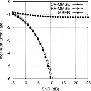
Fig. 2. BER comparison of three beamforming designs for the four-element array system supporting3users.

−4 −2

0 2

4

−4 −2 0 2 4 −1.5 −1 −0.5 0 0.5 1 1.5

Re[y] Im[y]

pdf

(a) CV-MMSE

−4 −2

0 2

4

−4 −2 0 2 4 −1.5 −1 −0.5 0 0.5 1 1.5

Re[y] Im[y]

pdf

(b) RV-MMSE

−4 −2

0 2

4

−4 −2 0 2 4 −1.5 −1 −0.5 0 0.5 1 1.5

Re[y] Im[y]

pdf

(c) MBER

Fig. 3. Conditional probability density functionsp(y|+ 1)(surfaces), marginal con-ditional probability density functionsp(yR|+ 1)(curves), signal subsetsY(+)

andY_R(+)(points) for the four-element array system supporting3users with SNR= 7dB. The beamformer weight vector is normalised to a unit length.

where

Q(u) =√1 2π

∞

u e−v

2

2 _{d v (21)}

and

g(q,+)(w) = sgn(b

(q) 1 )¯y

(q,+) R σn

√

wH_w . (22)

The BER can alternatively be computed based on the other subset

weight vector that minimises the error probability (20)

wMBER= arg min w

PE(w). (23)

The gradient ofPE(w)with respect towis given by

∇PE(w) =

1 2Nsb

√ 2πσn

√ wH_w

N_sb

q=1 e−

¯ y(q,+)

R

2

2σ2_nwHw

×sgnb(₁q)

¯

y(_Rq,+)w wH_w −x¯

(q,+)

, (24)

wherey¯R(q,+) = ℜ[w H_x¯(q,+)_]

∈ YR(+). Given the gradient (24), the optimisation problem (23) can be solved using a gradient-based algorithm [11],[14],[15]. Following the derivations presented in [11],[14], an adaptive implementation of the MBER solution can be realised using the LBER algorithm which takes the form of

w(k+ 1) =w(k) +µsgn(b1(k))

2√2πρn e−

y_R2(k)

2ρ2_{n x(k), (25)}

whereρnis the kernel width.

D. Comparison of Three Designs

The CV-MMSE solution minimises the MSE betweenb1(k)and y(k). Therefore, the associated conditional signal subsetY(+)_must have a symmetric distribution with respect toℜ[y]andℑ[y]axes. This imposes an unnecessary constraint and limits the achievable BER performance, since only the distribution ofYR(+) influences the BER performance. By removing the unnecessary constraint on yI(k), the RV-MMSE solution has more freedom in designing a more favourable distribution ofYR(+), leading to an improved BER. The minimum distance between the decision thresholdyR = 0 and the subset_YR(+) ultimately determines the BER. Minimising JrpMSE(w) does not guarantees maximising this minimum dis-tance. The MBER solution ensures that this minimum distance is maximised and, therefore, the MBER design generally provides a smaller BER than the RV-MMSE design. In terms of the compu-tational requirements per weight updating, it can be shown that the

-6 -5 -4 -3 -2 -1 0

-5 0 5 10 15 20 25

log10(Bit Error Rate)

SNR (dB) CV-MMSE RV-MMSE MBER

Fig. 4. BER comparison of three beamforming designs for the four-element array system supporting8users.

−6 −4 −2 0

2 4 6

−6 −4 −2 0 2 4 6 −1 −0.8 −0.6 −0.4 −0.2 0 0.2 0.4 0.6 0.8 1

Re[y] Im[y]

pdf

(a) CV-MMSE

−6 −4 −2 0

2 4 6

−6 −4 −2 0 2 4 6 −1 −0.8 −0.6 −0.4 −0.2 0 0.2 0.4 0.6 0.8 1

Re[y] Im[y]

pdf

(b) RV-MMSE

−6 −4 −2 0

2 4 6

−6 −4 −2 0 2 4 6 −1 −0.8 −0.6 −0.4 −0.2 0 0.2 0.4 0.6 0.8 1

Re[y] Im[y]

pdf

(c) MBER

Fig. 5. Conditional probability density functionsp(y|+ 1)(surfaces), marginal con-ditional probability density functionsp(yR|+ 1)(curves), signal subsetsY(+)

andY_R(+)(points) for the four-element array system supporting8users with SNR= 8dB. The beamformer weight vector is normalised to a unit length.

RV-LMS and LBER algorithms have a similar complexity, which is about half of the complexity required by the CV-LMS algorithm.

In order for the CV-MMSE solution to perform adequately, suf-ficient antenna array resource is required so that the interfering sig-nals can be cancelled. Thus, in order to ensure a correct separation ofYR(+)andY

(−)

xl(k)is CV or two-dimensional. Thus, the RV-MMSE design is ca-pable of supporting users up to twice the number of array elements. Therefore, for the RV-MMSE design, a system is overloaded only ifM >2L. The MBER design is no restricted by this limit and is capable of supporting more users.

-6 -5 -4 -3 -2 -1 0

-5 0 5 10 15 20 25

log10(Bit Error Rate)

SNR (dB) CV-MMSE RV-MMSE MBER

Fig. 6. BER comparison of three beamforming designs for the four-element array system supporting9users.

-0.1 0 0.1 0.2 0.3 0.4 0.5 0.6 0.7

-1 0 1 2 3 4 5

conditional pdf

Re[y] pdf states

(a) RV-MMSE

-0.1 0 0.1 0.2 0.3 0.4 0.5 0.6 0.7

-1 0 1 2 3 4 5

conditional pdf

Re[y] pdf states

(b) MBER

Fig. 7. Marginal conditional probability density functionsp(yR|+ 1)(curves) and

signal subsetsY_R(+)(points) for the four-element array system supporting9users with SNR= 15dB. The beamformer weight vector is normalised to a unit length.

IV. SIMULATIONSTUDY

The simulated system consisted of a four-element linear antenna array and supported up toM = 10users. Fig. 1 shows the array geometric structure and Table I lists the locations of users with re-spect to the antenna array. The simulated channel conditions were

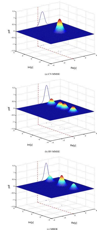
Ai = 1.0 +j0.0for all users and, therefore, SIRi = 0dB for all i. Fig. 2 compares the BER performance of the three beamformer designs when only the first 3 users were active. Given SNR= 7dB, Fig. 3 depicts the conditional PDFsp(y|+ 1), marginal conditional PDFsp(yR|+ 1), signal subsetsY(+)andY_R(+)for the three de-signs, where the beamformer weight vectorw was normalised to a unit length. It can be seen from Fig. 3 (a) that the distribution p(y|+ 1)is symmetric for the CV-MMSE solution. By contrast, the RV-MMSE and MBER designs are not restricted by this sym-metric constraint and spreadp(y|+ 1)more widely along theℑ[y]

axis, resulting in a more favourable distribution ofp(yR|+ 1). It can also be seen from Fig. 3 (a) that the CV-MMSE solution is able to correctly separateYR(−)andY

(+)

R and thus provide an adequate BER performance as seen in Fig. 2.

1e-5 1e-4 1e-3 1e-2

0 200 400 600 800 1000

Bit Error Rate

sample RV-LMS RV-MMSE LBER MBER

(a) Training

1e-5 1e-4 1e-3 1e-2

0 200 400 600 800 1000

Bit Error Rate

sample RV-LMS RV-MMSE LBER MBER

(b) Decision directed adaptation after 40-symbol training

Fig. 8. Learning curves of the adaptive RV-LMS and LBER algorithms averaged over 100 runs for the four-element array system supporting9users with SNR= 15dB. The step sizeµ= 0.005for the RV-LMS, the step sizeµ= 0.01and kernel varianceρ2

n= 2σ 2

nfor the LBER.

-6 -5 -4 -3 -2 -1 0

0 5 10 15 20 25 30

log10(Bit Error Rate)

SNR (dB) CV-MMSE RV-MMSE MBER

Fig. 9. BER comparison of three beamforming designs for the four-element array system supporting10users.

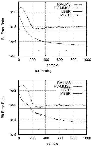
Fig. 6 compares the BER performance of the three beamformer designs when the first 9 users were active, while Fig. 7 shows the marginal conditional PDFsp(yR|+ 1)and signal subsetsYR(+)for the RV-MMSE and MBER designs, given SNR= 15dB. The RV-LMS and LBER algorithms were investigated, and Fig. 8 shows the convergence performance of the two adaptive algorithms averaged over 100 runs, given SNR= 15dB. In Fig. 8 (a), training was car-ried out over the whole length, while in Fig. 8 (b), after 40-symbol training, the decision directed (DD) adaptation was invoked by sub-stitutingˆb1(k)forb1(k).

Finally, Fig. 9 compares the BER performance of the three beam-formers when all the 10 users were active, while Fig. 10 shows the marginal conditional PDFsp(yR|+ 1)and signal subsetsY_R(+)for the RV-MMSE and MBER designs, given SNR= 20dB. Note that in Fig. 10 (a) a point ofYR(+)is in the wrong side of the decision thresholdyR= 0. It is seen that the RV-MMSE was no longer ca-pable of separatingYR(−)andY

(+)

R correctly and exhibited a BER floor, since the system was overloaded. By contrast, the MBER de-sign was still able to separateYR(−)andY

(+)

R correctly and provided a much better BER performance than the RV-MMSE design.

V. CONCLUSIONS

An alternative MMSE design has been considered for beamform-ing assisted BPSK receiver, which minimises the MSE between the real-valued desired output and the real part of the complex-valued beamformer output. This RV-MMSE design offers significant per-formance enhancement over the standard CV-MMSE design. A drawback of this RV-MMSE design, as compared with the CV-MMSE design, is that there exists no closed-form solution and nu-merical optimisation based on a gradient algorithm has to be used. It has been demonstrated that the RV-MMSE beamforming solution is capable of obtaining a BER performance that is close to the op-timal MBER solution for supporting BPSK users up to twice of the number of antenna array elements. The MBER design is capable of supporting more users than the RV-MMSE design. Adaptive al-gorithms for implementing these three beamforming designs have also been compared.

0 0.2 0.4 0.6 0.8 1 1.2

-1 0 1 2 3 4 5

conditional pdf

Re[y] pdf states

(a) RV-MMSE

0 0.2 0.4 0.6 0.8 1 1.2

-1 0 1 2 3 4 5

conditional pdf

Re[y] pdf states

(b) MBER

Fig. 10. Marginal conditional probability density functionsp(yR|+ 1)(curves)

and signal subsetsY_R(+)(points) for the four-element array system supporting10

users with SNR= 20dB. The beamformer weight vector is normalised.

REFERENCES

[1] J.H. Winters, J. Salz and R.D. Gitlin, “The impact of antenna diversity on the capacity of wireless communication systems,”IEEE Trans. Communications, Vol.42, No.2, pp.1740–1751, February/March/April 1994.

[2] J. Litva and T. K.Y. Lo,Digital Beamforming in Wireless Communications. London: Artech House, 1996.

[3] L. C. Godara, “Applications of antenna arrays to mobile communications, Part I: Performance improvement, feasibility, and system considerations,”Proc. IEEE, Vol.85, No.7, pp.1031–1060, 1997.

[4] A.J. Paulraj and C.B. Papadias, “Space-time processing for wireless communications,”IEEE Signal Processing Magazine, Vol.14, No.6, pp.49–83, 1997.

[5] R. Kohno, “Spatial and temporal communication theory using adaptive antenna array,”IEEE Personal Communications, Vol.5, No.1, pp.28–35, 1998.

[6] P. Petrus, R.B. Ertel and J.H. Reed, “Capacity enhancement using adaptive arrays in an AMPS system,”IEEE Trans. Vehicular Technology, Vol.47, No.3, pp.717–727, 1998.

[7] J.H. Winters, “Smart antennas for wireless systems,”IEEE Personal Communications, Vol.5, No.1, pp.23–27, 1998.

[8] P. Vandenameele, L. van Der Perre and M. Engels,Space Division Multiple Access for Wireless Local Area Networks. Boston: Kluwer Academic Publishers, 2001.

[9] J.S. Blogh and L. Hanzo,Third Generation Systems and Intelligent Wireless Networking – Smart Antenna and Adaptive Modulation. Chichester: John Wiley, 2002.

[10] A. Paulraj, R. Nabar and D. Gore,Introduction to Space-Time Wireless Communications. Cam-bridge: Cambridge University Press, 2003.

[11] S. Chen, N.N. Ahmad and L. Hanzo, “Adaptive minimum bit error rate beamforming,”IEEE Trans. Wireless Communications, Vol.4, No.2, pp.341–348, 2005.

[12] S. Chen, L. Hanzo, N.N. Ahmad and A. Wolfgang, “Adaptive minimum bit error rate beam-forming assisted QPSK receiver,” inProc. ICC 2004, 2004, Vol.6, pp.3389–3393. [13] S. Haykin,Adaptive Filter Theory, 3rd edition. Upper Saddle River, NJ: Prentice Hall, 1996. [14] S. Chen, A.K. Samingan, B. Mulgrew and L. Hanzo, “Adaptive minimum-BER linear

mul-tiuser detection for DS-CDMA signals in multipath channels,”IEEE Trans. Signal Processing, Vol.49, No.6, pp.1240–1247, 2001.