INTERNATIONAL
COUNCIL FOR
SCIENCE
INTERGOVERNMENTAL
OCEANOGRAPHIC
COMMISSION
UNESCO
WORLD
METEOROLOGICAL
ORGANIZATION
WORLD CLIMATE RESEARCH PROGRAMME
UNDERSTANDING THE ROLE OF THE INDIAN OCEAN
IN THE CLIMATE SYSTEM — IMPLEMENTATION PLAN
FOR SUSTAINED OBSERVATIONS
CLIVAR–GOOS Indian Ocean Panel and others
January 2006
Acknowledgements:
We gratefully acknowledge the assistance and comments received from P. Blouch, E. Charpentier, H. Cattle, M. Dengler, J. Gould, E. Harrison, H. Hendon, R. Lumkin, M. Merrifield, R. Molinari, S. Riser, B. Sloyan, N. Smith, A. Schiller, D. Walliser, J. Vialard, S. Wilson, K. Yoneyama, and the INSTANT group. Ray C. Griffiths carefully edited the final draft.
The work of the CLIVAR—GOOS Indian Ocean Panel is supported by the World Climate Research Programme, International CLIVAR Project Office, the Intergovernmental Oceanographic Commission Perth Regional Office, Indian Ocean GOOS, and the CSIRO Wealth from Oceans Flagship Programme.
CLIVAR is a component of the World Climate Research Programme (WCRP). WCRP is sponsored by the World Meterorological Organisation, the International Council for Science and the Intergovernmental Oceanographic Commission of UNESCO. The scientific planning and development of CLIVAR is under the guidance of the JSC Scientific Steering Group for CLIVAR assisted by the CLIVAR International Project Office. The Joint Scientific Committee (JSC) is the main body of WMO-ICSU-IOC formulating overall WCRP scientific concepts.
Bibliographic Citation
Table of Contents
Acknowledgements 2
Executive Summary and Recommendations 4
Introduction 9
Part 1 Research Issues and Operational Oceanograph 12
Background 12
1. Seasonal monsoon variability and the Indian ocean 13
2. Intraseasonal variability 14
3. Indian Ocean zonal dipole modeand El Niño–Southern Oscillation 16 4. Decadal variation and warming trends in the upper Indian Ocean 18
5. Southern Indian Ocean and climate variability 20
6. Circulation and the Indian Ocean heat budget 21
The cross-equatorial cell 22
Estimates of the rates of subduction and upwelling 22
Vertical structure at the equator 23
The subtropical cell 23
Interannual variability and climate relevance of the CEC anbd STC 23
Indonesian Throughflow 23
Deep meridional overturning cell 25
7. Biogeochemical cycling in the Indian Ocean 27
8. Operational oceanography 29
Part 2: Implementation of an integrated ocean observing system 31
9. The basin-scale mooring array 31
10. Argo profiling floats 36
11. Expendable bathythermographs 39
12. Surface drifters 41
13. Collaboration with Indian Ocean Tsunami Warning and Mitigation System 43
14. Biogeochemical observations 44
15. Process studies 47
16. Data management 49
Conclusion 50
Appendix 1 References 51
Appendix2 CLIVAR–GOOS Indian Ocean Panel members 60
Executive Summary and Recommendations
The circulation and transport of heat in the Indian Ocean is unique in many respects, compared to the Pacific and the Atlantic. The Asian landmass blocks the ocean in the north so that currents cannot carry tropical heat to higher latitude as the Atlantic and Pacific do. It also receives extra heat from the Pacific via the Indonesian Throughflow. The movement of heat around the ocean and exchange with the atmosphere is highly variable in time. As a consequence, the Indian Ocean plays a unique role in the variation of regional and global climate systems. The monsoon, or seasonal cycle, of southern Asia, East Africa and northern Australia interacts strongly with the Indian Ocean. Whereas the monsoon reversals of wind and rain recur each year, they do so with sufficient variability to create periods of relative drought and flood in large parts of the surrounding tropics, while teleconnections carry the climate anomaly into higher latitude regions on a global scale. The societal and economic impacts of these climate variations affect the lives of nearly two-thirds of the world’s population. The benefit to be derived from describing, understanding and predicting the coupled ocean–atmosphere behaviour in this region is potentially huge, but limited at the present time by a lack of observational data on the ocean. The climate variations in the atmosphere are relatively well known due to the systematic collection of weather data on a global scale since World War 2. The related climate-processes in the ocean however are poorly documented, particularly in the Indian Ocean, where the development of the Global Ocean Observing System has lagged behind that of the Pacific and the Atlantic. This report is concerned with developing a rationale and a plan for implementation of sustained, basin-scale observations in this data-deficient region.
Realizing the potential benefits will require acceptance of certain fundamental principles from the outset:
• Implementing basin-wide observations is too large a task for any one nation or agency to accomplish
alone. A multi-national approach is required. Agreement to use available national resources in a coordinated and cost-effective way is an essential part of achieving full implementation.
• Data should be distributed openly in a timely manner. There is a preference for communication of data in real time to make it available at climate analysis and prediction centers. Data management will follow the guidelines and policies of the Intergovernmental Oceanographic Commission and the World Climate Research Programme—CLIVAR project.
• Satellite observations of oceanic surface properties provide a framework for the observing system.
The in situ observations are complementary and provide subsurface information that complements and enhances interpretation of satellite data. While this report is concerned with in situ observations, we note that the research issues identified in Part 1 cannot be resolved without satellite data and we strongly recommend continued measurement of sea-surface temperature, sea level, ocean colour, wind, rain and cloud. Likewise, in situ observations are used to maintain calibration of satellite data. • Development requires close coordination between the research and the operational-oceanography
communities. Some of the observations in this plan have already been partially implemented by operational programmes in the Global Climate Observing System (GCOS) and Global Ocean Observing System (GOOS); for example, the ship-of-opportunity expendable-bathythermograph programme and surface drifters. Full implementation requires close coordination among the Ocean Observation Panel for Climate (OOPC), the CLIVAR Global Synthesis of Observations Panel (GSOP), the International Argo Science Team (IAST) and the IOC–WMO Joint Committee for Oceanography and Marine Meteorology (JCOMM).
• An integrated observing system using a variety of instruments is required to address the diversity of time- and space-scalesof climate-relevant variability.
While this report is primarily concerned with oceanographic measurements, the meteorological measurements (particularly at moorings) will be extremely valuable to data assimilation issues concerned with weather forecasting and reanalysis efforts. At present there are few such measurements in the Indian Ocean and this lack of information prevents accurate initial condition determination of weather forecasts and limits reanalysis efforts.
The rationale for the observing system from an oceanographic perspective is discussed in Part 1 of the report. The science-drivers are improved description, understanding, modelling and ability to predict:
• Seasonal monsoon variability and the Indian Ocean • Intraseasonal variability
• Indian Ocean zonal dipole mode and El Nino–Southern Oscillation • Decadal variation and warming trends in the upper Indian Ocean • Southern Indian Ocean and climate variability
• Circulation and the Indian Ocean heat budget (including Indonesian Throughflow, shallow and deep
overturning cells)
• Biogeochemical cycling in the Indian Ocean.
Also, operational oceanography will provide a range of products, including routine daily to weekly maps of temperature, salinity and currents to support maritime safety, fisheries and management of the marine environment, as well as initialization of coupled models for seasonal climate prediction. Part 1 reviews the present state of knowledge and recent progress for each of these topics, and identifies the science questions and issues that have to be addressed with new observations to improve capability for prediction.
The design and implementation of an integrated observing system is discussed in Part 2. The instruments available for large-scale ocean monitoring are moorings (for subsurface temperature, salinity and currents and surface weather variables that determine the fluxes of heat and fresh water), Argo floats for subsurface temperature and salinity, expendable bathythermograph (XBT) lines, surface drifters for sea-surface temperature and current and sea-level stations.
The key new element of the observing system is a basin-scale mooring array, which is essential to capture the seasonal monsoon variability and intraseasonal disturbances. The fast intraseasonal time-scale requires continuous time-series, which is only possible with mooring technology. The array provides well resolved data on the interannual variations, particularly with regard to mixed-layer dynamics. The array is made up of 34 moorings for measurement of temperature, salinity and basic weather variables; 5 Acoustic Doppler Current Profilers for equatorial and coastal boundary currents and 8 moorings for enhanced measurement of surface fluxes in different climatic zones. The array is designed to resolve the most energetic variations in the ocean and interactions with the atmosphere. The current profilers are located where geostrophy cannot be used to estimate currents. The flux moorings provide data to calibrate flux estimates from satellite data; and they are located in regions where flux climatology is poorly known. The report provides complete technical data for the design of the mooring array.
Several merchant shipping routes were equipped with expendable bathythermographs (XBT) to measure temperature to a depth of 750 m during the 1980s as a component of individual research projects. The activity was transferred to national programmes after 1995, and is now coordinated by the Ship-of-Opportunity Implementation Panel (SOOPIP) under auspices of the IOC–WMO Joint Committee for Oceanography and Marine Meteorology (JCOMM). The XBT network in the Indian Ocean was never fully implemented. XBT lines are effective for monitoring specific ocean structures that affect climate, such as the upwelling zones off Java, Somalia, the Lakshadweep Dome and the thermocline ridge near 10°S. These are regions known to have strong ocean–atmosphere interactions. Combined with Argo floats the high-resolution XBT lines are effective to cut the upper ocean up into regions where the net transport, in or out, the interior heat and freshwater storage and the surface fluxes can be monitored, providing a method to understand the role of ocean dynamics in climate variations. The Indian Ocean Panel critically reviewed the XBT lines in preparing this report, with regard to scientific justification, potential impact on future research and feasibility of implementation. The high-priority lines were determined to be IX01, IX08, IX09N/IX10E, IX12, IX22 and PX-02 for the so-called frequently repeated (FRX) sampling mode; and IX1, IX15/IX21, and possibly IX10 for the high-density (HDX) sampling mode. The intraseasonal variation is strong at the north end of IX1 and the deployment of moorings is not advisable in this region, owing to intensive fishing activity; enhanced sampling to better resolve the fast time-scale is recommended for this line.
IOC and WMO through JCOMM sponsored an international workshop to organize implementation of the high-priority western Indian Ocean XBT lines in October 2005. The workshop was unique in that it brought together researchers, operators, shipping managers and customs officials. The outcomes were: improved protocols for shipping XBT’s across national boundaries (which in the past was an impediment in the Indian Ocean region), identification of ships for presently unoccupied lines, a USA-India effort to occupy IX08, identification of a need for capacity building in the region and consensus to work toward full implementation of the XBT network.
The International Buoy Programme for the Indian Ocean (IBPIO) was formally established at a meeting in La Réunion in 1996. IBPIO is the primary body for coordinating multinational activities to implement surface drifting buoys. The number of drifters measuring surface velocity and SST in the Indian Ocean north of 40°N is typically about 60, whereas about 160 are required for full coverage at the standard sampling density. The primary uses of drifter data are reduction of the bias error in satellite SST measurements; documentation of large-scale surface current patterns and their role in heat transports; and, potentially, validation of surface currents in ocean models. Full implementation of the array at least at the standard sampling density is recommended. A well planned re-seeding programme will be required to maintain the array north of the equator because drifters are pushed out of the region by summer monsoon winds. The standard sampling density was determined with regard to the goal of calibrating satellite SST. A re-evaluation of the sampling density is required for measurement of surface current, particularly as forecasting of surface current in operational ocean models comes into common practice.
The international response to the Indian Ocean tsunami disaster in December 2004 is the rapid development of an Indian Ocean Tsunami Warning and Mitigation System. This development will potentially have numerous synergies with the development of the climate observing system discussed above, particularly if the warning system addresses the multiple hazards of tsunami, tropical cyclone, storm surge, coastal flooding and other potential marine hazards. The potential synergies include logistics of maintaining deep-sea mooring sites, shared ship time, protection from vandalism, coordinated development of instrumentation packages, fail-safe communication systems and a long-term commitment to maintain the sites in the open ocean. There is obvious synergy in the maintenance of real-time tide-gauge/sea-level stations. Maintenance of a long-term datum to observe sea-level rise is an essential requirement for the climate observing system and needs to be guaranteed in the implementation of tide gauges for tsunami warning. Real-time sea-level stations are needed to facilitate the maintenance of continuous sea-level records and to validate satellite altimetry data in operational ocean models.
developed instruments on ships of opportunity, and biogeochemical sensors on the basin-scale mooring array and Argo floats.
This report provides a survey of planned and future regional process studies that will be carried out within the background of the sustained basin-scale observing system.
Data management is not addressed explicitly here; however, an approach to developing a plan based on existing resources is recommended.
The report concludes with the idea that, in designing an integrated observing system for the Indian Ocean, and in particular in identifying the need for a basin-scale mooring array, focus has been placed on the Indian Ocean zonal dipole mode and the pronounced intraseasonal variation that exists in the tropics, features that have strong climatic impacts on the surrounding land masses. The proposed observing system calls for Argo floats, XBT lines and surface drifters in the subtropical southern Indian Ocean and at higher latitude; however, these observations alone are not likely to adequately capture all aspects of subtropical variability, particularly in the boundary currents and major frontal zones. Therefore an extension of the system, such as additional mooring arrays, may be needed in the future as more is learned from the initial, sustained observations and process studies.
Recommendations (numbered according to the section of the report where they appear)
Recommendation Intro.1 The agencies contributing to the integrated observing system accept, follow and further develop the principles given in the Introduction.
Recommendation 9.1 The agencies contributing to the mooring arrayagree to the mooring plan and, recognizing that implementation depends on national resources, agree to negotiate changes to the plan with the other agencies doing mooring work.
Recommendation 9.2 Recognizing that ship-time is the key resource needed to implement the array, the agencies agree to optimise the use of their vessels to maintain the array when they are available and to proceed to a multi-agency agreement on ship-time as soon as possible.
Recommendation 9.3 Increase the number of moorings deployed at recommended sites as soon as possible, with a view to full implementation of the array within five years.
Recommendation 10.1 As a minimum, the planned 3×3 Argo Programme in the Indian Ocean should be completed and maintained.
Recommendation 10.2 INCOIS identify and publicize deployment opportunities, including research-vessel opportunities during routine mooring-maintenance cruises and process studies, as well as contacts to enable air-deployment or deployments from chartered ships in remote regions that are not regularly crossed by commercial shipping.
Recommendation 10.3 Model/observing-system experiments suggest that the sub-seasonal Indian Ocean temperature variability recovered from sampling at 5-day intervals does not represent a significant improvement over 10-day sampling. Continuation of 10-day sampling is recommended until further studies of the integrated sampling strategy.
Recommendation 10.4 Actions should be taken to ensure that Argo floats are continuously maintained in key centres of action: e.g. Java/Sumatra upwelling region, SEC/SECC ridge (western region), Bay of Bengal, where divergent currents tend to disperse them.
Recommendation 11.1 Implement the full XBT network in accordance with the guidelines given below. Recommendation 11.2 Increase sampling on IX1 to weekly sections to better resolve intraseasonal variability, including four high-density sections per year to measure Indonesian Throughflow; increase the number of thermosalinograph sections.
Recommendation 11.5 Data from all the XBT lines should be submitted to JCOMM/OPS annually.
Recommendation 12.1 Full implementation of the surface drifter array at least at 5° latitude/longitude spacing for calibration of satellite SST data is strongly recommended, particularly with regard to the area north of the equator where clouds often interfere with passive measurements and where very active re-seeding is required to maintain the array, owing to strong southward surface currents.
Recommendation 12.2 A study to determine an appropriate sampling strategy for surface currents is needed. Recommendation 13.1 The CLIVAR community needs to establish formal links with the tsunami community to take advantage of possible synergy in developing the Indian Ocean Tsunami Warning and Mitigation System and the Global Climate Observing System.
Recommendation 13.2 The IOTWS will be more robust and useful if it addresses the multiple hazards of tsunami, tropical cyclone, storm surge and coastal flooding. This will enhance links to GCOS.
Recommendation 13.3 Enhance the network of sea-level stations to allow real-time transmission of data to a tsunami warning centre, without diminishing the stations’ capability to build a long-term record of a well maintained datum for the determination of sea-level rise.
Recommendation 14.1 Full implementation of repeat hydrographic sections for the Indian Ocean, with carbon, transient tracer and related biogeochemical measurements.
Recommendation 14.2 Instrumentation of all surface-flux reference sites in the Indian Ocean mooring array, with biogeochemical sensors and assessment of the need to instrument other surface moorings in the array. Recommendation 14.3 Develop biogeochemical instrumentation on all suitable research ships and XBT lines in the Indian Ocean.
Recommendation 14.4 Work in collaboration with the biogeochemical community to assess and, where possible, deploy Argo floats with biogeochemical instrumentation.
Recommendation 14.5 Organize a workshop in 2006 to bring together the biogeochemical and physical interests in developing the Indian Ocean observing system (IndOOS)
Introduction
Of the three major oceans – Pacific, Atlantic, and Indian – the Indian is the only one that is not open to the northern subtropical regions. This is a consequence of the presence of the Asian landmass restricting the Indian Ocean to south of about 25°N. The Indian Ocean is also the only ocean with a low-latitude opening in its eastern boundary. The unique geography has important implications for the oceanic circulation physics, and consequently for climate and the biogeochemistry of the ocean, giving the Indian Ocean many unique features. It cannot transport heat gained in the tropics to the higher northern latitudes, as the Pacific and Atlantic do, mainly via their western boundary currents. It gains additional heat from the tropical Pacific via the Indonesian Throughflow. Heat is carried southward along the western coast of Australia toward the southern subtropics. The Indian Ocean consequently has a unique system of three-dimensional currents and interactions with the atmosphere that redistribute heat to keep the ocean approximately in a long-term thermal equilibrium. The Indian Ocean interacts strongly with the surrounding land masses resulting in the well known monsoons, or seasonal cycle, of southern Asia, East Africa and northern Australia. Short-term imbalances and irregularity in oceanic heat storage give the climate system a tendency to vary at a broad range of time-scales from a few weeks (intraseasonal variation) to years and decades. The variation in the atmosphere is documented and at least partially understood, due to the longstanding collection of weather data. Sustained in situdata from the ocean are however scarce, and an understanding of the role of ocean dynamics in the regional climate system is consequently limited. In this report we will first review the scientific issues and questions concerned with regional ocean–atmosphere interaction, and then lay out an implementation plan for sustained, in situoceanic observations to address these issues.
From the outset, we recognize the following principles:
• Implementing basin-wide observations is too large a task for any one nation or agency to accomplish
alone. A multi-national approach is required. Agreement to use available national resources in a coordinated and cost-effective way is an essential part of achieving full implementation.
• Data should be distributed openly in a timely manner. there is a preference for communication of data in real time to make it available at climate analysis and prediction centres. Data management will follow the guidelines and policies of the Intergovernmental Oceanographic Commission and CLIVAR.
• Satellite observations of ocean-surface properties provide a framework for the observing system. The in situ observations are complementary and provide subsurface information that complements and enhances interpretation ofsatellite data. While this document is concerned with in situ observations, we note that the research issues identified in Part 1 cannot be resolved without satellite data and we strongly recommend continued measurement of sea-surface temperature, sea level, ocean colour, wind, rain and cloud. Likewise, in situ observations are used to maintain calibration of satellite data. • Development requires close coordination between the research and operational-oceanography
communities. Some of the observations in this plan have already been partially implemented by operational programmes in GCOS and GOOS; for example, the ship-of-opportunity expendable bathythermograph programme and surface drifters. Full implementation requires close coordination with the Ocean Observation Panel for Climate (OOPC), the CLIVAR Global Synthesis of Observations Panel (GSOP), the International Argo Programme’s Science Team (IAST) and the IOC–WMOJoint Committee for Oceanography and Marine Meteorology (JCOMM).
• An integrated observing system is required to address the diversity of time- and space-scalesof climate-relevant variability. This means that a variety of instruments will be used, each in an appropriate way considering the time-scale that has to be resolved and the physical or biological parameter to be measured.
More than anything else, international and inter-agency cooperation and good-will are required to successfully implement the Indian Ocean observing system (IndOOS). The above principles are intended to provide a basis for the common endeavour.
Recommendation Intro.1 The agencies contributing to the integrated observing system accept, follow and further develop the above principles.
full agreement on the modes of access to exclusive economic zones has not been reached. The political realities have historically had an impact on data sharing. Nevertheless, the threat to countries in the region from natural hazards is recognized now, and may lead to rapid improvement. The Argo Programme and the TAO/Triton Programme in the Pacific will serve as examples of data management for development of the Indian Ocean observing system (IndOOS). Countries and research groups participating in these Programmes have agreed to the open exchange of data. This applies equally to the real-time (GTS and ftp) data stream (over 90 per cent available within 24 h) and to delayed-mode data. It is recommended that these standards of timeliness and openness be applied to all Indian Ocean observations.
While this report is primarily concerned with oceanographic measurements, the meteorological measurements (particularly at moorings) will be extremely valuable to data assimilation issues concerned with weather forecasting and reanalysis efforts. At present there are no such measurements in the Indian Ocean and this lack of information prevents accurate initial condition determination of weather forecasts and limits reanalysis efforts.
Part 1 of this report updates the Indian Ocean research issues identified by Godfrey et al. (1995) and the CLIVAR Research Plan sections G2 and G4 prepared in 1997 (
http://eprints.soton.ac.uk/35512/01/014_
Init_Imp_Plan.pdf
). The science-drivers discussed here are improved description, understanding, modellingand ability to predict:
• Seasonal monsoon variability and the Indian Ocean • Intraseasonal variability
• Indian Ocean zonal dipole mode and El Niño–Southern Oscillation • Decadal variation and warming trends in the upper Indian Ocean • Southern Indian Ocean and climate variability
• Circulation and the Indian Ocean heat budget (Indonesian Throughflow, shallow and deep overturning
cells)
• Biogeochemical cycling in the Indian Ocean
Operational oceanography and programmes developing a capability for ocean-state estimation (e.g. Global Ocean Data Assimilation Experiment
http://www.bom.gov.au/bmrc/ocean/GODAE/
) also require insitu data. The uses of operational products range from initialization of coupled climate models for seasonal prediction to information for maritime safety, fisheries and management of the marine environment. With these applications in mind, all of the dominant space and time-scales of variation need to be observed. For the Indian Ocean the fast, upperocean variability associated with intraseasonal disturbances is a challenge that has to be addressed by the observing system.
Part 2 is concerned with implementation of the elements that make up the basin-scale integrated in situ observing system. The planned basin-scale system is in Figure 1 (page 61), including fixed moorings, Argo floats, XBT lines, surface drifters and tide gauges, which are addressed in separate sections. Monitoring of boundary regions is not yet planned. It is worth mentioning here, although not covered in detail in this report, that multi-year regional monitoring is needed in the Arabian Sea (ASEA), the Bay of Bengal (BOB), the Indonesian Throughflow (ITF), the western (WBC) and eastern boundary currents (EBC) and deep equatorial currents indicated by a double arrow (+). Pilot projects in some of these regions are also discussed in Part 2.
The mooring array is the critical new element in Indian Ocean observations, required to understand the energetic intraseasonal variation in the upper-ocean, as well as mixed-layer thermodynamic processes in interannual variability. The array spans the tropical zone and provides well resolved time-series of surface weather parameters and upper-ocean temperature and salinity. A subset of the array will be equipped to measure equatorial currents and to estimate surface heat and freshwater fluxes. Argo floats, XBT lines and surface-drifters are already partially implemented in the Indian Ocean. This report sets out the plan for what we consider the full implementation required to understand the longer time-scales of variation, from seasonal climate to multi-decadal climate change.
Part 1 Research Issues and Operational Oceanography Background
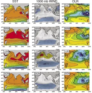
The monsoon is the characteristic feature of Indian Ocean climate. The topography of the Asian landmass is dominated by the Tibetan Plateau which has an area of about a million square kilometres and an average height of about 5 km. The plateau acts as an elevated heat source for the atmosphere during the northern summer. The heating in spring, combined with a build-up of moisture over the northern Indian Ocean, triggers processes that lead to large seasonal changes in wind and out-going long wave radiation (OLR) indicative of precipitation in Asia (Fig. 2, page 61). During January the equatorial rain-band, i.e. the Inter-Tropical Convergence Zone (ITCZ), is located primarily in the southern hemisphere. The region north of the ITCZ then experiences northeasterly trade winds and that to the south, the southeasterly trades. This distribution of wind and precipitation is similar to that over other tropical regions of the world. During northern summer the ITCZ virtually covers the entire Bay of Bengal, the surrounding lands, and the eastern Arabian Sea. The winds in the north turn into strong southwesterlies, while the southeasterlies persist in the south. The wind speed is much greater than that during the northern winter. This seasonal reversal of winds and rainfall is the well known monsoon, a special feature of the region with profound implications for both the ocean and the people who live under its influence, about 60% of the population of the world.
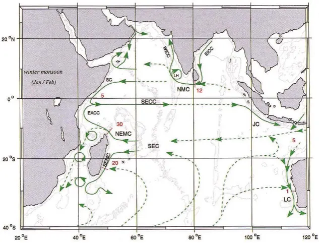
Whereas the reversals of wind and rain recur each year, they do so with sufficient variability to create periods of relative drought and flood in large parts of southern Asia, East Africa and northern Australia. The societal impact of the variations is very large. The anomalies are often associated with strong, intraseasonal disturbances— weather patterns that evolve systematically over a period of three to four weeks—that can determine the character of an entire season of rainfall. A challenge for modern climate research is to understand how the ocean responds to the atmosphere and feeds back the heat and moisture that together govern the intraseasonal to interannual variation. This is the primary reason that sustained observations in the ocean are needed. Process studies of relatively short duration in the past, and ocean models, together provide a qualitative view of the ocean’s response to monsoon forcing (Schott and McCreary, 2001). The precipitation and wind stress depicted in Figure 2 bring about a response (Fig. 3a,b, page 62) that is distinctly different in the northern and southern parts of the Indian Ocean. A subsurface hydrothermal front near 10°S (Wyrtki, 1971) separates the monsoon-driven, northern region from the steadier southern region. The circulation in the North is strongly seasonal, and the currents experience a complete reversal from January–February (Fig. 3a) to July–August (Fig. 3b). During the transition between the monsoons, May and October, the equatorial Indian Ocean exhibits eastward jets, so-called Wyrtki Jets (Wyrtki, 1973). The highly seasonal circulation north of 10°S is a superposition of tropical and coastal locally and remotely forced waves with frequencies that range from intraseasonal to interannual. The waves lead to strong seasonally reversing currents, the most prominent being the following: the Somali Current along the coast of Somalia; the monsoon currents in the mid-basin (Shankar et al., 2002); and the West and East India Coastal Currents (Shetye and Gouveia, 1998).
South of about 10°S the direction of the currents remains approximately unchanged from season to season (Fig. 3a,b), and steady state ocean circulation theory (Sverdrup-theory), which takes Indonesian Throughflow into account (Godfrey and Golding, 1981), explains much of the structure of currents and density. The Agulhas Current, the Mozambique Current eddies and the East Madagascar Current form a complex western-boundary current system along the East African coast.
In summary, geography of the Indian Ocean sets the stage for a highly variable, 3-dimensional ocean circulation that responds to the monsoons. While the monsoons recur each year, their irregularity at a range of time-scales from weeks to years depends on feedback from the ocean in ways that are not fully understood. The geography also impacts the biogeochemistry of the region, leading to an ocean environment that has unique features. Part 1 is concerned with the outstanding research issues that need to be addressed with observations to advance our understanding of the role of the Indian Ocean in the climate system and its predictability. The issues addressed in the next 8 sections are:
1. Seasonal monsoon variability and the Indian Ocean 2. Intraseasonal variability
6. Circulation and the Indian Ocean heat budget (Indonesian Throughflow, shallow and deep overturning cells)
7. Biogeochemical cycling in the Indian Ocean 8. Operational oceanography
1. Seasonal monsoon variability and the ocean
Despite the critical need for accurate and timely monsoon forecasts, our ability to predict seasonal conditions has not changed substantially over the last few decades. Statistical methods have shown that while there are periods of high correlation between El Niño–Southern Oscillation (ENSO) and monsoon variation, there are decades where there appears to be little or no association at all (e.g. Torrence and Webster, 1999), making statistical prediction unreliable. Why this first-order predictability disappears for long periods of time is not known.
The critical need for seasonal prediction cannot at this time be filled by coupled, numerical modelling either. Dynamical prediction is still in its infancy and severely handicapped by the inability of models to simulate either the mean monsoon structure, or its year-to-year variation (Sperber and Palmer, 1996; Gadgil and Sajani, 1998), or the intraseasonal (20–50 day period) band which controls a very large percentage of the precipitation (Slingo et al., 1996; Waliser et al., 2003a, 2003b). What is the reason for the general failure of models to forecast monsoon variation? Clearly, there are model problems associated with characterization of convection. At the same time, it is apparent that many of the climate phenomena are coupled with ocean thermodynamics and hydrodynamics. This is clear for seasonal and interannual variability (e.g. Webster et al., 1998) and highly probable for sub-seasonal or intraseasonal variability (see section 2). Yet our current knowledge of the ocean– atmosphere interactions is limited by a lack of ocean data, particularly data relevant to the fast variability of temperature, salinity and currents in the mixed layer. In particular, for the Indian Ocean, incorporating the mixed-layer thermodynamics of thin, low-salinity layers at the surface into models is a challenge. Also, surface “weather” data such as near surface winds, temperature, humidity and radiation are lacking in the Indian Ocean, in comparison to the Pacific and Atlantic. Future research to understand the ocean–atmosphere interactions will place a high reliance both on model capabilities and the observations needed for understanding processes. Despite the limited capability for prediction described above, recent progress increases our confidence that the capability can be improved (Walliser, 2005a). Better data for initialization of the numerical models will in itself improve predictions. Beyond that, there are physical reasons to expect improvement. Empirical schemes (Walliser et al., 1999; Lo and Hendon, 2000; Wheeler and Weickmann, 2001;Webster and Hoyos, 2004) have shown that regional precipitation characteristics are predictable with considerable accuracy 20–30 days in advance. Why models tend to show less skill than empirical techniques is less known, although there is some evidence that it is associated with problems in convective parameterization. For the interannual time-scale, a recent series of empirical studies have shown that the relationships between Indian Ocean SST and Indian rainfall are stronger than portrayed in earlier studies if the ENSO signal is properly addressed (Clark et al., 2000) The SST–monsoon relationship is apparent in the seasonally stratified persistence of SST anomaly across the tropical Indo-Pacific basin (Fig. 4, page 63). The Pacific Ocean has a strong persistent minimum in the boreal spring, known as the “predictability barrier”, but shows persistence of several months after ENSO events begin, typically in June. The pattern in the Indian Ocean is quite different. Strong persistence occurs from the end of the boreal summer to the late spring of the following year, consistent with the idea that there is a biennial component in the Indian Ocean SST and monsoon rainfall in Asia and Australia (Meehl, 1997). The structure of persistence suggests that Indian Ocean thermodynamics is somewhat independent of the Pacific Ocean, in ways that are not yet simulated in coupled climate models.
The small SST variation is thought to be related to advection by ocean currents. Despite biases (see below), the annual mean heat flux into the northern Indian Ocean has been estimated at about +50 to +70 Wm-2 in
numerous studies in the past (Hastenrath and Lamb,1978; Hsiung et al., 1989; Oberhuber, 1988, Hastenrath and Greischar, 1993). After considering how this intake of heat can be balanced, Godfrey et al. (1995, p. 12) concluded:
“... on an annual average there is positive heat flux into the Indian Ocean, nearly everywhere north of 15° S. The integral of the net heat influx into the Indian Ocean over the area north of 15° S ranges between 0.5–1.0×10¹⁵ W, depending on the climatology. Thus, on the annual mean, there must be a net inflow of cold water (into the North Indian Ocean), and a corresponding removal of warmed water, to carry this heat influx southward, out of the tropical Indian Ocean. ...” Thus it is inferred that oceanic heat transport represents the only means that allows the large net annual surface heating of the northern Indian Ocean to be removed without raising the SST substantially.
Similarly, the annual cycle of net surface flux is large enough to cause a temperature change of 7°C during the year, if all the heat were stored in a 50-m mixed layer (Webster et al., 1998), but the large amplitude does not develop. A hypothesis based on models is that the unique 3-dimensional, basin-scale circulation of the Indian Ocean stabilizes the annual mean temperature and dampens the annual cycle (Loschnigg and Webster, 2000), as discussed further in section 7.
Clearly, knowing the climatological surface heat balance of the Indian Ocean is necessary to understand the monsoons. However, there are large differences (biases, 20–50 Wm-2) between presently available estimates
(Godfrey et al., 1995; L. Yu, personal communication). This should not be surprising as the surface heat balances are the relatively small sums of large terms, and data in the Indian Ocean are sparse. Furthermore, these large terms are obtained from empirical rules some of which are not precisely understood and which produce large errors in the estimates.
Given the problems in the prediction of monsoons, and in the light of the recent discoveries regarding the structure of Indian Ocean variation (see sections 2 and 3), a number of questions about the monsoons need to be addressed, and they will require an improved observing system:
(i) What factors determine the phase and the amplitude of the monsoon annual cycle? In particular, why is the amplitude of the SST variation so small?
(ii) What factors control the interannual rainfall variation of the South Asian monsoon so that the persistent multi-year anomalies and large excursions from long-term means are rare?
(iii) What factors produce the intraseasonal oscillation of the monsoon system which, in turn, produces seasons of drought or flood?
(iv) In particular, what is the role of ocean circulation and thermodynamics in the monsoon and the intraseasonal time-scale?
(v) To what extent is the monsoon a coupled ocean-atmosphere phenomenon? For example, do the correlations between Indian Ocean SST and monsoon rainfall indicate the existence of coupled modes? (vi) What are the modes of interannual to decadal variability in the region and how do they interact? 2. Intraseasonal variability
Progress in understanding the intraseasonal variability in oceanic structure and currents was recently reviewed in depth by Kessler (2005), in a volume that is dedicated to an extensive review of atmospheric MISO and MJO. He described the essential oceanic physics as follows, “[The events] affect the ocean through three main mechanisms: increased evaporation, the generation of equatorial jets and waves that produce advective changes remotely, and enhanced mixing and entrainment….these responses are proportional to the wind speed
u, u2and u3, respectively, and therefore depend very differently on the background wind and the structure of its
variance. Much of the forcing by tropical intraseasonal oscillations…occurs over the warm pools of the Indian and west Pacific Oceans where the thermocline is usually deeper than the mixed layer. Thus, the near-surface density structure is relatively unconstrained by large-scale ocean dynamics and can easily be modulated by the winds and the heat and moisture fluxes…, providing the opportunity for air–sea feedbacks, nonlinear effects, and the retention of an oceanic memory of previous forcing. The dynamic response depends on the thickness of the accelerating layer, which is a function both of the background stratification and of local precipitation and mixing. Thus a principal focus…is the factors controlling the upper-ocean stratification under rapidly changing windspeed and precipitation sufficient for salinity variation to determine the mixed-layer depth. The correlation of intraseasonal variation of solar shortwave forcing with the wind fluctuations can also lead to significant effects on mixed-layer temperature structure.”
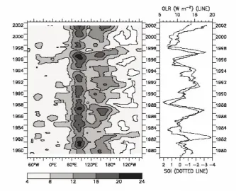
The core, the most energetic region of global, interannual variability of MISO and MJO (Fig. 5 page 63, left panel) is in the central, eastern Indian Ocean near 90°E (Kessler, 2001) Whether or not intraseasonal variability in the core region plays an active, causal role in the ENSO cycle is still a matter of debate. Interannual indices of the variability indicate that the correlation over longer time-series is not high (Hendon et al., 1999; Slingo et al., 1999); however, activity in the core region was at a maximum just before the 1982 and 1997 El Niños (Fig. 5, right panel). Further discussion of the atmospheric side of intraseasonal variability is beyond the scope of this report; interested readers are referred to the comprehensive review by Lau and Walliser (2005).
The oceanic response to MISO/MJO is strongly affected by the boundary of the Indian Ocean. Strong westerly winds during intraseasonal events generate eastward currents in a ~300-km band on either side of the equator and the Kelvin waves that carry the response to the eastern boundary (Walliser et al. 2003c, 2004; Schiller and Godfrey, 2001; Masumoto et al., 2005). The Kelvin waves reflect as coastal waves and propagate around the Bay of Bengal into the Arabian Sea (Shetye and Gouveia, 1998). The regional currents and variations in oceanic structure are strong and have important societal impacts on the coastal communities, such as impact on fishing. The MISO in the atmosphere sometimes propagates northward into the Bay of Bengal, under the influence of SST patterns, affecting monsoon rainfall. There are very energetic responses in currents, salinity structure and subsurface fronts in the Bay of Bengal (Webster et al., 2002); however, the role of ocean dynamics in the northward propagation of MISO is not known.
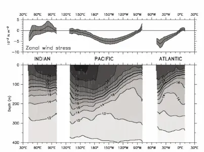
The mean structure of the thermocline and the pycnocline (Fig. 6, page 64) sets the background state on which the basin-scale intraseasonal variability develops, and distinguishes the Indian Ocean from other regions. The thermocline in the eastern Indian Ocean is deep, in comparison to the Pacific and the Atlantic, primarily as a consequence of the opening to the Pacific through Indonesia (see section 6). Also, unlike the other oceans, the wind stress along the equator is predominantly eastward, giving the thermocline a downward slope toward the east. The deep thermocline shields the surface from thermocline dynamics and allows the formation of a large, deep pool of surface water with a temperature exceeding 28°C. Heavy runoff into the Bay of Bengal and rainfall over Indonesia form widespread, thin layers of low-salinity water, creating the so-called “barrier layer” (e.g. Qu and Meyers, 2005), within the thick surface isothermal layer. This structure leads to a complex mixed-layer dynamics that has to be documented, understood and modelled in order to predict SST (Slingo, personal communication; 2004 AAMP meeting).
The MISO and MJO are associated with strong fluctuations in surface heat fluxes, primarily evaporation and solar radiation, and they generate large (~1°C), well known fluctuations in SST (e.g. Webster et al., 2002; Harrison and Vecchi, 2001; Duvel et al, 2004). The role of horizontal advection on SST is more subtle, but has been observed at times in the western Pacific (Kessler, 2005), for which there are adequate data. The vertical mixing usually cools the surface layer, but can at times warm it in the presence of a barrier layer (Du et al., 2005). The challenge for future research on the intraseasonal time-scale in the Indian Ocean is to understand how oceanic processes generate SST and feedback to the atmosphere by modulating convection.
temperature and salinity structure and direct measurement of equatorial currents are needed. The Japanese equatorial mooring program in the eastern equatorial Indian Ocean since November 2000 (Masumoto et al., 2005) has demonstrated that each new mooring brings about a quantum increase in description of the complex structure and time scales of variability in this region. Already the results provide us with a new perspective on importance of the energetic intraseasonal variability of currents, its strong correlation with the wind variability and other weather variables and the impact of wind-driven currents on structure of the mixed layer and barrier layer. A deeper understanding of the role of the ocean in MISO and MJO requires implementation of a basin-scale mooring array in the tropical Indian Ocean.
Some of the critical scientific questions that will be addressed by the observing system are:
• How much of the SST variation is controlled by local, surface fluxes and can be simulated with a
1-D (vertical) model of the mixed layer, including barrier-layer dynamics and the low-salinity water lenses?
• Under what circumstances do horizontal currents, baroclinic waves and mixing play a role? • Which, if any, oceanic processes are related to the MISO and MJO convection?
3. Indian Ocean zonal dipole mode and El Niño–Southern Oscillation
A multitude of forces shape the structure of interannual SST patterns in the Indian Ocean, rendering it more complex than tropical SST variations elsewhere. Strong monsoons and intraseasonal events affect the tropical SST on a large scale, as discussed in sections 1 and 2. Also, coupled ocean-atmosphere modes of variability affect the SST pattern.
The IOZDM pattern was first clearly identified in two seminal papers in Nature (Webster et al.,1999; Saji et al.; 1999), although aspects of it had been noted in earlier publications. The papers stimulated a vigorous, scientific debate concerning (1) whether or not IOZDM was a local, passive oceanic response to atmospheric ENSO teleconnections, and (2) whether or not IOZDM could maintain itself by positive feedback through ocean–atmosphere interaction within the Indian Ocean. At one extreme of the debate, some authors argued that IOZDM was a statistical artifact of the methods used to identify it. A summary of the debate is published in the CLIVAR Exchanges newsletter, (Allan et al., 2001; Yamagata et al., 2002). The proponents of IOZDM argued that it is a coupled mode inherent in the Indian Ocean, although at the time only one paper documenting observed variation in the thermocline had been published (Rao et al., 2002). Variation in the depth of the thermocline is a critical factor in coupled climate-modes because the slow dynamics of thermocline adjustment to changing wind conditions (such as Kelvin and Rossby waves) gives the mode persistence and predictability for lead-times of a few to several months. The thermocline process also allows the development of a delayed, negative feedback that returns the coupled ocean–atmosphere toward a normal state.
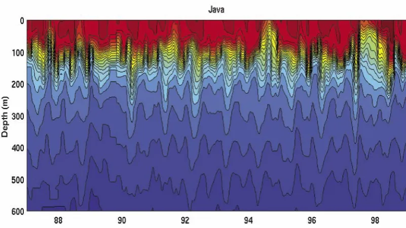
Subsequent observational studies increasingly clarified the role of thermocline variation in IOZDM and raised new, important research questions. These studies found that seasonal upwelling off Java played an important role in the formation of IOZDM SST anomaly (Fig. 8, page 65) (Wijffels and Meyers, 2004). Also like ENSO, thermocline depth anomalies propagate as Kelvin and Rossby waves and play an important role in the evolution of the SST anomalies (Rao et al., 2002; Feng and Meyers, 2003; Yamagata et al., 2004). Since thermocline variations have a consistent dipole structure in the tropical Indian Ocean, and the structure is often not evident in the SST anomaly, we need to study the surface-layer heat budget to understand why SST is sometimes decoupled from thermocline anomaly during extremes of IOZDM, in contrast to the more consistent relationship in the Pacific Ocean during ENSO extremes. Strong variation in depth of the thermocline is observed in both poles of IOZDM (Wijffels and Meyers, 2004; Xie et al., 2002), but it is not always the dominant factor in generating SST anomaly, particularly in the west.
Climate models suggest a hypothesis on the mechanism that allows IOZDM to grow. The relation between thermocline depth, SST, rainfall and surface winds during IOZDM, inferred from observational analysis is reproduced successfully (with some important caveats) in coupled climate models (e.g. Murtugudde et al., 2000; Gualdi et al., 2003; Fischer et al., 2005; Yamagata et al., 2004; Cai et al., 2005). The models suggest that upwelling and thermocline depth in the Java/Sumatra region are key processes that control ocean–atmosphere interaction during growth. Stronger upwelling increases the zonal SST gradient toward the west; and the SST gradient in turn feeds back to produce a stronger easterly wind.
Like ENSO, the IOZDM has climate impacts on regional and global scales. Rainfall anomaly in many of the Indian Ocean rim countries is correlated with IOZDM, with largest impacts observed over equatorial East Africa and Indonesia (Saji and Yamagata, 2003). Moderate impacts are noted over Sri Lanka (Lareef et al., 2003) and Australia (England et al., 2005). The IOZDM may affect the Indian monsoons (Ashok et al., 2001; Gadgil et al., 2003), but the relation is confounded in the presence of ENSO.
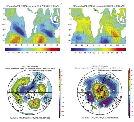
Recent studies have identified a global correlation to subtropical surface air temperatures in the southern hemisphere (Saji and Yamagata, 2003). Figure 9, page 65, depicts the correlation of IOZDM with temperature anomalies in the southern hemisphere. Interestingly, strong and significant correlations are found in the subtropical land-surface temperature of the southern hemisphere underlying the subtropical jet stream axis in accordance with the linear theory of Rossby-wave propagation. Further analysis by Saji et al. (2005) has shown that this relationship is indeed quite strong and statistically robust. It seems that both IOZDM and ENSO can generate Rossby-wave trains that affect South America, the South Atlantic and southern Africa (e.g. Kiladis and Mo, 1988; Mo and Paegle, 2001; Colberg et al., 2004). IOZDM may also impact temperature variation over parts of Europe, northeast Asia and North America (Saji and Yamagata, 2003). Guan and Yamagata (2003) found that the intense heat-wave conditions during the summer of 1994 over Japan and northeast Asia were related to a strong IOZDM.
Unlike ENSO, the present-day coupled dynamical prediction systems for seasonal climate cannot predict the SST anomaly of IOZDM with the same level of skill as for ENSO SST anomaly. This surprising result suggests that we need a much better understanding of the dynamics and thermodynamics of the observed IOZDM, the associated mixed layer and barrier layer dynamics and their representation in models. Key research questions that can be addressed with better ocean observations are:
circulation and structure involved in the waxing and waning of the correlation between monsoon rainfall and ENSO?
• What is the relationship between ocean circulation, depth of the thermocline, depth of the barrier layer,
SST and surface fluxes during IOZDM episodes?
• What mechanisms control the triggering, growth and decay of IOZDM?
• Will the prediction skill in respect of Indian Ocean SST improve with better observations for the
initialization of a prediction run?
4. Decadal variation and warming trends in the upper Indian Ocean
The CLIVAR Initial Implementation Plan in 1998 noted that the data base for Indian Ocean variability and change is so poor that knowledge of decadal, oceanic variability in the Indian Ocean was almost unknown. However, analysis of historical SST and SLP data sets (Allan et al., 1995) provided evidence of interdecadal variation in the strength and location of the southern Indian Ocean anticyclone. With improved processing of the historical SST data (Rayner et al., 2003; Smith and Reynolds, 2004; NOAA/CIRES Climate Diagnostics Center, 2003) and oceanographic data (Levitus et al., 2005), improved climate modelling and continuation of the WOCE repeat-hydrography sections, there has recently been progress in identifying regional decadal variability and trends. The Indian Ocean is recognized now as a centre of decadal to multi-decadal SST variation and change that has an impact on regional and global climate.
Human-induced climate change is debatably the most important environmental issue facing humanity in the twenty-first century, and is certainly linked to the great societal issues of our time—availability of water and energy. Increasingly, in the years and decades to come, governments and industries will have to make policies and management decisions that guide the societal response to future climate. Research on climate change has to provide a solid scientific foundation for these policies and decisions. A major uncertainty emerging at this time is the linkage between natural climate variability (monsoons, MISO, ENSO, IOZDM) and climate change as a result of fossil-fuel burning. It is now widely recognized that future climate change may express itself as changes in the physics of the natural modes of variability due to changes in the background state on which the natural variations develop. The change in background state in turn changes the frequency and intensity of extreme events. Perhaps more than any other reason, sustained ocean observations are needed to understand the linkages between climate variability and change, to model them appropriately and to produce reliable predictions of future climate for policy and management purposes.
Much of what is known at the present time about decadal to multi-decadal variation and change in the ocean comes from the SST records, which have been much better monitored, in the twentieth century, than any other oceanographic property. The tropical Indian Ocean and the subtropics off western Australia have warmed over this period, and the rate of warming has accelerated substantially during the last 30 years (Fig. 10, page 65). There is growing evidence that these changes play a key role in shaping important features of twentieth-century climate variability and change that have had huge impacts, from the drying trend of the African Sahel (Giannini et al., 2003) to the Pacific decadal variability (Deser et al., 2004) to the North Atlantic Oscillation (Hoerling et al., 2004).
Within the Indian Ocean region, the monsoon circulation has steadily weakened over the last 50 years (Sperber et al., 2000) and seems to be related to the Indian Ocean warming and the reduction in land–sea contrast in temperature. Also, the MISO/MJO have been more active in the last 20 years (Slingo et al., 1999), consistent with the tropical warming. Both the weakened monsoon circulation and the more active intraseasonal variability are supported by the new 40-year ECMWF reanalysis (Slingo, personal communication). Southwestern Australia has experienced a large decrease in rainfall and a 40 per cent reduction in inflow to the Perth water supply during the past 30 years (IOCI, 2001). Although research has not specifically related the reduction to Indian Ocean SST, the impact of the large-scale warming in the eastern Indian Ocean (Fig. 10) has not been tested in models, nor is its relationship to oceanic processes known.
mixing that determine SST. Vastly improved, in situ estimates of surface fluxes—heat and fresh water—will be required, as well as sustained measurement of currents, mixed-layer and thermocline processes.
Levitus et al. (2005) have devoted a large effort during the past decade to assembling all the available subsurface ocean data. Their records show that world ocean heat content (0–3000 m depth range) has increased 14.5×10²² J
between 1955 and 1998 (Fig. 11, page 66). Levitus et al. (2005) point out that the global ocean warming may be underestimated owing to insufficient ocean data in some regions. Their records also show cooling periods interrupting the warming trend, indicative of the interplay between human effects, natural variability and, possibly, volcanic effects.
The increasing heat content in the ocean leads to a measurable sea-level rise. A number of nations in the Indian Ocean region are particularly susceptible to sea-level rise, changing frequency and intensity of cyclones and the associated changes in the impacts of extreme sea-level (storm surge) events. These events will occur more frequently as sea level rises. The more severe cyclonic storms will lead to more frequent generation of devastating surges in sea level along the coastline. The Bay of Bengal is already one of the regions of the world most badly affected by coastal storm surges. The severe damage that has been caused here can be appreciated from the list given by Ali and Chowdhury (1997) of the worst storm surges on record anywhere in the world. Of the 34 disasters they listed in which death toll was 5,000 or more, 26 occurred along the coast of the Indian peninsula. Of these, 15 were along the coast of Bangladesh. An episode in 1970 killed 500,000 in Bangladesh; another in 1991 killed 138,000 in the same country. The loss of life in a 1994 event came down to ~200 because of improved early-warning methods based on better storm-forecast models together with the availability of elevated shelters that allowed people on low land to flee the flood waters. Yet still there is an increasing threat due to sea-level rise and climate change, and an opportunity to take greater protective measures.
Recent reconstructions of global and Indian Ocean sea level (Church et al., 2004, 2005) for the twentieth century were constrained by the very few long records available and their poor spatial distribution. These reconstructions suggested a minimum rate of sea-level rise in the central equatorial Indian Ocean and along the northwest coast of Australia in the latter part of the twentieth century and a maximum in the equatorial eastern Indian Ocean. The changing frequency of extreme sea-level events as a consequence of multi-decadal sea-level rise is an active area of research. The changing risk needs to be documented in particular for the Indian Ocean.
Model projections of level rise for the twenty-first century reveal quite different patterns of regional sea-level rise (Gregory et al., 2001). However, as the different models have quite different regional distributions, sea-level data with adequate datum control are required. A better understanding of the oceanic mechanisms that produce warming of the subsurface and validation of these mechanisms in models are required to move toward consensus on the estimates of regional sea-level rise.
Decadal variability is superimposed on the multi-decadal trends discussed above. Much of the decadal variation in oceanic structure observed to date is often attributed to natural processes, but the relationship of these modes to human-induced climate change is not yet known. Decadal variation in the interannual correlations between the SST-based indices of IOZDM and ENSO has been documented by Clark et al. (2000) who found alternating decades of high (~0.5) and low correlation. Annamalai et al. (2005) investigated the decadal changes of interannual correlation using a suite of ocean-model experiments concentrating on the decadal variation of thermocline depth. They started from the hypothesis that preconditioning of stratification in the eastern equatorial Indian Ocean by the Indonesian Throughflow (an oceanic teleconnection) might play a role related to Pacific decadal variability. They concluded that the reason for IOZDM events to occur independently of ENSO events is that a decadal shallow thermocline in the eastern Indian Ocean favours the development of occasional cold (positive) IOZDM events. From singular value decomposition they showed that the thermocline was particularly shallow during 1952–1971 and 1990–1996, matching periods of strong IOZDM developed independently of ENSO. The shallow thermocline was transmitted from the Pacific through the Indonesian passages. Annamalai et al. (2005) proposed that this was an effect of advection by the Indonesian Throughflow. They also found an atmospheric teleconnection that produced wind over the equatorial Indian Ocean favouring the shallow thermocline in the East. It is, however, fair to state that the role of decadal ocean circulation in climate is still poorly understood and needs to be a focus of future research.
be related (Smith et al., 2000) to the rainfall and pressure. Over South Africa and neighbouring countries, a nearly bi-decadal signal in rainfall has long been known (Tyson et al., 1975), but whose driving mechanism is not understood. Reason and Rouault (2002) showed that this rainfall variation was related to changes in atmospheric circulation and SST over the Indian Ocean that modulate southern African rainfall ondecadal scales.
The heat content in the upper 300 m of the southern Indian Ocean, according to the compendium by Levitus et al. (2005), has relatively large decadal fluctuations super-imposed on the multi-decadal warming trend. In contrast, the variability in the northern Indian Ocean is much smaller on these time-scales, consistent with earlier analyses of wind and pressure data (Allen et al., 1995). The changes in the atmosphere seem to drive the heat-content variation. The shallow subtropical and equatorial overturning cells (see section 6) are important to the maintenance of the heat content in the upper few hundred metres of the southern and northern Indian Ocean, respectively. An important question is whether the southern overturning cell fluctuates more than the cross-equatorial overturning cell on decadal time-scales and thus contributes to the observed heat-content changes. It is necessary to examine the potential coupling of the tropical southern Indian Ocean with the atmosphere and its impact on decadal and longer-term variability. Based on satellite observations of wind stress and sea level, Lee (2004) suggested a near-decadal decrease of the overturning rate in the subtropical cell by about 7 Sv from 1992 to 2000, which is nearly 70 per cent of its average strength; yet no evidence of significant change in the cross-equatorial overturning cell was found during this period. Sustained in situ and satellite observations are indispensable to the assessment of the potentially important role of the Indian Ocean circulation in the regions’ decadal and longer-term climate variability, as discussed further in section 6.
Analysis of historical hydrographic sections illustrates the need for sustained observations and the inadequacy of historical data to document decadal and longer-term trends in Indian Ocean circulation. A careful comparison of sections in the International Indian Ocean Expedition in the early 1960s with a transoceanic section in 1987 identified basin-wide changes in temperature, salinity and oxygen below the mixed layer near 32°S during the 25 years from 1962 to 1987 (Bindoff and McDougall, 2000). The changes are explained by a surface warming in the higher-latitude source regions of Sub-Antarctic Mode Water and by increased precipitation in the source region of Antarctic Intermediate Water. They seem to be consistent with the expected response to human-induced global warming (Banks and Bindoff, 2002). However a new trans-Indian section across 32°S reveals that thermocline mode waters have changed back toward the structure of the 1960’s (Bryden et al., 2003). The shift back to the pre-1987 conditions again indicates the interplay between natural variability and global warming. These studies illustrate again the need for sustained in situ and satellite observation of subsurface properties to better understand and model natural decadal variation and its relationship to human-induced climate change.
5. Southern Indian Ocean and climate variability
The eastern and western boundaries of the southern Indian Ocean extend only to relatively low latitudes (about 34.5oS for South Africa and 43oS for Tasmania). This geometry has important consequences for the variability
of circulation, since it implies efficient communication with the South Atlantic, South Pacific and Southern Oceans. The southern Indian Ocean is also linked to the tropics, and therefore is influenced by the Indonesian Throughflow, currents generated by the monsoons and the tropical modes of interannual variability (ENSO and IOZDM; see section 3). The unique currents and SST of the southern Indian Ocean in turn are related to climate variability and change over the surrounding continents.
The evolution of SST in the tropical Indian Ocean during an El Niño year (see section 3), is complemented by a tropical to mid-latitude SST anomaly pattern by the end of the year (Cadet, 1985; Allan et al., 1996; Reason et al., 2000). Although it has long been known that there are significant rainfall impacts on East Africa and southern Africa at this time (e.g. Ogallo, 1988; Lindesay, 1988), skill in forecasting the rainfall for individual events is less than in regions closer to the equatorial Pacific, pointing to the potential contribution of other factors, such as variability in the southern Indian Ocean or the South Atlantic Ocean and regional land–sea interactions.
al., 2002, 2003; Reason, 1998) and potentially also downstream in southern Australia (Reason, 2001). Heat transported southward by the Leeuwin Current and lost to the atmosphere influences the climate of Western Australia (e.g. Gentilli, 1991; Reason, 1996), creating a region quite different from the west coasts of other continents by its lack of significant coastal upwelling and a hyper-arid coastal desert. While Chile and southern Africa have significant coastal upwelling and coastal desert, Western Australia has a relatively moist climate and no upwelling.
Although early work (Walker, 1990; Jury et al., 1993) showed the importance of SST variation in the Agulhas Current region for South African summer rainfall, recently a larger, dipole-like SST anomaly pattern in the subtropical southern Indian Ocean has been found to be associated with rainfall variation over large parts of southern Africa poleward of about 15°S (Reason, 2001; Behera and Yamagata, 2001). The pattern is oriented SW–NE, with one pole south of Madagascar and the other west of Western Australia. Analysis of these events using a coupled model (Suzuki et al., 2004) showed the importance of wind-driven latent-heat flux anomaly for their generation which tends to be confined to the summer, since that is when the mixed layer is sufficiently shallow. Sometimes a similar dipole-like pattern also exists simultaneously in the South Atlantic (Fauchereau et al., 2003; Hermes and Reason, 2005) pointing to a near-hemispheric atmospheric forcing pattern that involves shifts in the wave-number (3 or 4) circulation pattern in the mid-latitude southern hemisphere and in the Antarctic Oscillation (Fig. 12, page 66). Analysis of an OGCM forced by 1948–1999 NCEP re-analyses (Hermes and Reason, 2005) suggests decadal variations between the patterns in the Atlantic and Indian Oceans (Fig. 13, page 67). When the South Atlantic and southern Indian Ocean events are in phase, there may be a link to the ENSO-induced Pacific South America (PSA) pattern. The SST anomaly appears to arise mainly from surface heat-flux anomaly driven by the atmospheric forcing, with contributions to the western pole also coming from Rossby waves generated by the anomalous winds and from modulations of the South Equatorial Current.
Further modelling work (particularly with coupled models) is needed to fully understand and assess the predictability of the observed rainfall variation over southern Africa and southern Australia. The oceanography of the southern Indian Ocean during phases of ENSO, IOZDM (and their teleconnections to higher latitude), the Antarctic Oscillation (or Sub-Antarctic Annular Mode) and the dipole-like SST patterns in the subtropical southern Indian Ocean needs to be documented by sustained observations. Ultimately the impacts of regional ocean-atmosphere modes on the climate of neighbouring land-masses need to be better understood, and predicted if possible.
The scientific questions and issues that need addressing by the observing system include:
• Determining the relationships between the regional atmospheric forcing (modulations of barometric
pressure in the southern Indian Ocean) and the larger-scale modes, such as ENSO and the Antarctic Oscillation
• Does the southern Indian Ocean have a particular tendency (e.g. due to its geometry or the
relationship of the hemispheric atmospheric circulation to the land-masses or the unique ocean currents) to evolve dipole-like SST patterns in the subtropics–mid-latitudes?
• What are the feedbacks between these SST patterns and the atmosphere? • What is the predictability of these SST patterns?
• What is the relationship between the southern Indian dipole-like SST variation and that occurring
in the South Atlantic and the South Pacific?
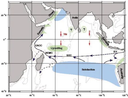
6. Circulation and the Indian Ocean heat budget
Embedded within the system of upper-layer currents, as described in the Background to Part 1 (Fig. 3a,b), is a unique, three-dimensional circulation that plays an important role in the surface-layer heat budget, and consequently a role in the climate system (Schott and McCreary, 2001). The annual average circulation is illustrated in Fig. 14, page 67. The seasonal variation was shown in Fig. 3. Subduction in a large region south of 20°S (Fig. 14, blue) feeds water into the Indonesian Throughflow and the South Equatorial Current, primarily within the depth range of the thermocline. Part of this water crosses the equator in boundary currents near East Africa and joins the circulation in the northern Indian Ocean. Thermocline water comes to the surface in as many as seven upwelling zones (Fig. 14, green) in the tropical zone. Ekman currents in the surface layer (Fig. 14, red) carry water back across the equator to near 20°S.