1
Sampling effects on the quantification of sodium content in infant formula using laser 1
induced breakdown spectroscopy (LIBS) 2
3
Xavier Cama-Moncunilla, *, Maria Markiewicz-Keszyckaa, Raquel Cama-Moncunilla, Yash 4
Dixita , Maria P. Casado-Gavaldaa, Patrick J. Cullena,b, Carl Sullivana 5
6
a) School of Food Science and Environmental Health, Dublin Institute of Technology, Cathal 7
Brugha St, Dublin 1, Ireland 8
9
b) Department Chemical and Environmental Engineering, University of Nottingham, UK 10
11
*Corresponding author 12
Xavier Cama-Moncunill 13
School of Food Science and Environmental Health, 14
Dublin Institute of Technology, Cathal Brugha St, Dublin 1, Ireland 15
2 Abstract
18
In the present work, laser-induced breakdown spectroscopy (LIBS) was employed to predict 19
the sodium content of infant formula (IF) over the range of 0.5–4 mg Na/g. Calibration 20
models were built using partial least squares regression (PLS), correlating the LIBS spectral 21
data with reference Na contents quantified by atomic absorption spectroscopy (AAS). The 22
aim of this study was to demonstrate the ability of LIBS as a rapid tool for quantifying 23
sodium in IF, but also to explore strategies concerning the acquisition of measurements with 24
LIBS. A range of different pre-processing techniques, measuring depths (repetition of laser 25
shots) and accumulations were evaluated in terms of PLS performance. The best calibration 26
model was developed using the third-layer spectra normalised by the H I 656.29 nm emission 27
line, yielding a coefficient of determination (R2) of 0.93, and root-mean-square errors 28
(RMSE) of 0.37 and 0.13 mg/g for cross-validation and validation, respectively. 29
30
Industrial relevance 31
Improving productivity and robustness of manufacturing processes, yet satisfying increasing 32
concerns and strict regulations on the quality and safety of infant products could be achieved 33
through the introduction of optical analytical techniques with real-time capabilities during 34
processing. In this paper, LIBS is proposed as a potential cost-effective screening tool that 35
can provide fast elemental composition analysis of IF. Specifically, the application of LIBS 36
and multivariate data analysis for predicting sodium content over a range in conformity with 37
regulatory guidelines is discussed in this work. 38
39
Keywords 40
3 1.Introduction
42
Infant formula (IF) is an industrially produced food intended as a substitute for breast milk. 43
IFs are typically based on cow’s milk, and followed by several adjustments and addition of 44
ingredients in order to bring the composition closer to that of human milk (Blanchard, Zhu, & 45
Schuck, 2013). Infancy is a crucial period of growth and development, hence IF’s 46
composition (e.g. fat, proteins, minerals, etc.) and manufacturing practices are strictly 47
regulated by national authorities to ensure the safety and nutrient profile of infant formula 48
products (Jiang, 2014; Montagne, Van Dael, Skanderby, & Hugelshofer, 2009). 49
Sodium is an essential mineral; it is the main cation in extracellular fluid playing a vital role 50
in the regulation of osmolarity, acid-base equilibrium, active transport across cells and 51
membrane potential (Guo, 2014). Although a minimum intake is indispensable for healthy 52
functioning, an excessive consumption of sodium in the human diet is related to higher blood 53
pressure and an increased risk of developing cardiovascular diseases (Masotti, Erba, De Noni, 54
& Pellegrino, 2012; Tamm, Bolumar, Bajovic, & Toepfl, 2016). With regard to infancy, 55
studies have also associated an excessive sodium intake with increased blood pressure in the 56
later stages of life, indicating that blood pressure may track with age (Campbell et al., 2014; 57
John et al., 2016). 58
Conventional well-established methods for mineral analysis in infant formula include atomic 59
absorption spectroscopy (AAS), inductively coupled plasma optical emission spectroscopy 60
(ICP-OES) and inductively coupled plasma mass spectroscopy (ICP-MS) (Poitevin, 2016). 61
These methods, despite their high sensitivity and accuracy, generally require time-consuming 62
and laborious sampling procedures and the use of chemical reagents such as acids and gases, 63
as well as an associated high cost of consumables (e.g. argon) (Wu & Sun, 2013). 64
Laser-induced breakdown spectroscopy (LIBS) is an analytical technique based on optical 65
4
vaporise, atomise and ionise a small part of the target’s material. As a result, plasma arising 67
from the sample surface is generated from which photons are released form the excited 68
species in the plasma returning to their ground state levels of energy which can be analysed 69
with spectrometers to infer the elemental composition of the sample (Cremers & Radziemski, 70
2013). LIBS, yet recent in the area of food analysis, has gained remarkable popularity in the 71
last few years with an increase in the number of publications and extensive reviews 72
concerning food samples (Maria Markiewicz-Keszycka et al., 2017; Sezer, Bilge, & Boyaci, 73
2017). The advantages that LIBS offers compared to the conventional methods are its speed, 74
a relatively low cost, little to no sample preparation and elemental surface mapping 75
capabilities (Dixit et al., 2017; Kim, Kwak, Choi, & Park, 2012). Further attractive features 76
include: remote sensing, as it constitutes an entirely optical technique, and suitability for on-77
/at-line applications, altogether allowing the technology to be considered a potential process 78
analytical technology (PAT) for qualitative and quantitative chemical analysis (Cullen, 79
Bakalis, & Sullivan, 2017) (for PAT literature the reader is referred to: Misra et al., 2015; van 80
den Berg et al., 2013). Nonetheless, LIBS also has limitations or drawbacks, especially 81
concerning quantitative analyses. Some of these limitations include signal fluctuations on a 82
shot-to-shot basis (Tognoni & Cristoforetti, 2016) and difficulties in establishing good 83
calibration curves due to strong matrix effects (Ferreira et al., 2010; Lei et al., 2011). Several 84
publications evaluating and discussing strategies with the goal of overcoming such problems 85
can be found in the literature (dos Santos Augusto, Barsanelli, Pereira, & Pereira-Filho, 2017; 86
El Haddad, Canioni, & Bousquet, 2014; Jantzi et al., 2016). 87
In this study, LIBS and multivariate data analysis with partial least squares regression (PLS) 88
was employed to predict the sodium content of IF samples. In order to provide for reference 89
Na contents, atomic absorption spectroscopy (AAS) was used. The aim of this study was to 90
5
relevant to IF manufacturing, offering a means for industries to rapidly verify target mineral 92
contents. Furthermore, strategies concerning the acquisition of measurements with LIBS were 93
explored, namely the repetition of laser shots on a single location. Such an approach 94
examines the impact of measuring the inner layers of the sample and, whether to accumulate 95
laser shots or use the spectra collected from a single layer. 96
2.Material and methods 97
2.1.Sample preparation
98
Commercial powdered IF and follow-on formulas (formulas intended for children over 6 99
months of age) were acquired from a local supermarket in Dublin, Ireland. Lactose (α-lactose 100
monohydrate ≥ 99 %) and sodium chloride (NaCl ≥ 99 %) were purchased from Sigma 101
Aldrich (St. Louis, MO, USA). 102
Samples with varying content of sodium were prepared by blending IF with sodium chloride 103
or lactose, whether the goal was to increase or decrease the sodium content in the mix. In 104
total, 7 samples were obtained, including one sample which consisted only of IF. The 105
selected range of sodium was approx. from 0.5 to 4 mg/g (concentrations corresponding to 106
the lowest and highest Na content samples, respectively). This range was intended to cover 107
the regulatory sodium levels provided by the Codex Alimentarius Commission (Codex, 108
2007). Constituents of the mixtures (IF, NaCl and lactose) and follow-on formulas were 109
ground and pre-mixed using a laboratory blender (8011G, Waring Laboratory Science, CT, 110
USA) equipped with rotatory stainless-steel blades for 2 minutes to ensure there were no 111
aggregates occurring in the powders, with the goal of improving subsequent blending 112
performance. Dry mixing was then carried out using a laboratory V-mixer (FTLMV-1L&, 113
Filtra Vibracion S.L., Spain) for 20 minutes. In order to ensure reproducibility, two 114
independent batches were prepared (batch 1 and batch 2). Each batch was composed of the 115
6
employed for PLS modelling, and 2 validation samples (V1, V2) to test the robustness of the 117
models. In addition to these validation samples, 2 different follow-on formula brand samples 118
(V3, V4) were used to assess the ability of the calibrations for predicting mineral content in 119
infant products with different formulations. 120
For LIBS analysis, samples were pelletized by pressing approx. 400 mg of each sample using 121
a manual hydraulic press fitted with a 13 mm pellet die (Specac Ltd., UK) at 10 tons for 3 122
minutes. Pellets were prepared in triplicates (3 replicates per sample), giving a total number 123
of 48 pellets. The two batches of samples were measured on different days. 124
2.2.Atomic absorption spectroscopy (AAS)
125
AAS was selected as the reference method for sodium quantification in IF mixtures. Na 126
contents were established using a Varian 55B AA spectrometer (Varian, United States) 127
following the standard method 985.35 for mineral determination in IF of the AOAC (Official 128
Methods of Analysis of AOAC International) with slight modifications. Approximately 1.5 g 129
of each sample was transferred to a crucible in triplicates (3 replicates). Crucibles were 130
placed on a hot plate and heated until smoking ceased. Organic matter was then decomposed 131
by dry ashing in a muffle furnace at 525°C for 4 h. Ashes were dissolved in 50 mL 1 M nitric 132
acid. A further dilution step was required to bring concentrations within the linear range of 133
the instrument (0–1 ppm). 134
Calibration curves were established by using aqueous standards prepared from a commercial 135
sodium stock solution (Sodium standard for AAS – 1,000 mg/L, Sigma-Aldrich). Sodium 136
absorbance was measured at 589 nm with a slit width of 0.5 nm. All replicates and batches 137
7
2.3.LIBS instrumentation and measurements
139
2.3.1.Instrument set-up
140
LIBS spectra were recorded using a LIBSCAN-150 system (Applied Photonics Ltd, UK) 141
described in a previous publication (X. Cama-Moncunill et al., 2017). The system was fitted 142
with a 150 mJ Q-switched Nd:YAG laser (Ultra, Quantel laser, MT, USA) operating at 1064 143
nm and a pulse duration of 5 ns, coupled to six fibre-optic spectrophotometers (AvaSpec, 144
Avantes spectrometers, Netherlands) covering the wavelength range of 181–904 nm. 145
Moreover, the system was equipped with a miniature CCD camera which enabled the 146
monitoring of the measurements. 147
For the experiments, plasma emission was analysed with a delay time of 1.27 µs and an 148
integration time of 1.1 ms. The laser was operated with a firing repetition rate of 1 Hz. 149
2.3.2.Sampling method
150
Pellets were measured individually using a sample chamber equipped with a three-axis 151
translation stage (Applied Photonics Ltd, UK) which facilitated the acquisition of spectra at 152
multiple locations of the pellet surface, that is, 100 locations following a 10×10 grid pattern. 153
Spectral acquisition was carried out by recording 5 consecutive laser shots (depth 154
measurements) at each of the 100 locations, giving a total number of 500 measurements per 155
pellet. Data resulting from these consecutive laser shots can be considered as spectra 156
corresponding to 5 different layers of the pellets, i.e. the repetitive firing of the laser at the 157
same location causes the ablation of the outer material penetrating and allowing to measure 158
deeper into the sample (Cremers & Radziemski, 2013). 159
Spectral data collected from the 5 laser shots were stored separately in order to assess the best 160
layer from which to build the sodium quantification model, and to allow subsequent 161
8
2.4.Data analysis
163
Data analysis was performed with R (R Core Team, 2014) using the R package “pls” (Mevik, 164
Wehrens, & Liland, 2015) for conducting PLS (partial least squares regression), as well as 165
other in-house functions. 166
Firstly, the average of the LIBS spectra collected at multiple locations was calculated for 167
each layer, resulting in 5 spectra per pellet. Data was then divided into a training data set 168
(N=30) and a test set (N=12), additionally the follow-on formula extra validation samples 169
(N=6) were tested. Prior to PLS modelling, combinations of different pre-processing 170
techniques and normalisation methods were applied to the spectra with the aim of reducing 171
the signal fluctuations due to extraneous sources of variability and to minimize any matrix 172
effects (Sobron, Wang, & Sobron, 2012). Specifically, the techniques explored were: baseline 173
correction (R package “baseline”), second derivative and standard normal variate (SNV). 174
Spectral normalisation using other approaches, including normalisation by an internal 175
standard and the Euclidean norm, were also explored. 176
PLS calibration models using the different pre-processing techniques were developed for 177
each of the 5 layers of the pellets. The performance of each model was evaluated by the 178
leave-one-out root-mean-square error of cross-validation (RMSECV) technique, as well as 179
the root-mean-square error of prediction (RMSEP). The wavelength range used for the 180
modelling was limited to 560–825 nm since this region encompassed the main Na emission 181
lines, while decreasing the total number of variables that do not contain useful peaks 182
(Moncayo, Manzoor, Rosales, Anzano, & Caceres, 2017). 183
In order to provide for a comparison between the accumulated and non-accumulated shots, 184
spectra corresponding to the different layers were summated to one another so that 2, 3, 4 and 185
9
out, and their resulting performances were compared to those of the single-layer-spectra 187
models. 188
The limit of detection was computed according to the pseudounivariate approach (LODpu) for 189
PLS models as proposed in a publication elsewhere (Allegrini & Olivieri, 2014) in 190
accordance with IUPAC official recommendations. LODpu calculation was performed as 191
shown in Eq. 1. 192
𝐿𝑂𝐷𝑝𝑢 = 𝑆3.3
𝑝𝑢 [(1 + ℎ0 𝑚𝑖𝑛+
1
𝐼) 𝑣𝑎𝑟𝑝𝑢] 1
2 ⁄
(1)
193
where Spu is the slope of the pseudounivariate line, ho min is the minimum leverage when the 194
analyte concentration is zero, I the number of samples employed for calibration, and varpu is 195
the variance of the regression residuals. 196
3.Results and discussion 197
3.1.AAS
198
In AAS, the accuracy of the results relies heavily upon the calibration curve established from 199
reference standard solutions of the desired element. Good calibration curves were obtained 200
rendering values for the coefficient of determination (R2) ≥ 0.99. Sodium contents of the IF 201
samples determined with AAS, expressed in mg/g, are shown in Table 1. 202
3.2.LIBS spectral features
203
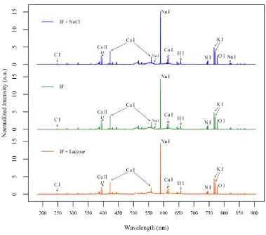
An initial exploratory analysis of the LIBS spectra was conducted in order to determine the 204
principal differences among the samples studied. For comparison purposes, the averaged 205
spectra of pellets corresponding to the lactose-IF mixture (C1, approx. 0.5 mg Na/g), pure IF 206
(C2, approx. 1.3 mg Na/g) and the sodium chloride-IF mixture (C5, approx. 3.7 mg Na/g) are 207
shown in Fig. 1. In the figure, several of the most important spectral lines of elements 208
occurring in the spectra can be seen. The main element emission lines in the spectra were 209
identified using the NIST database (Kramida, Ralchenko, Reader, & NIST ASD team, 2016). 210
10
612.22; 616.22 nm, H I 656.29 nm, N I 744.23; 746.83 nm, K I 766.49; 769.90 nm, O I 212
777.19 nm and Na I 589.05; 589.59 nm. Moreover, three Na I lines were identified at 568.26, 213
568.82 and 819.48 nm. Other possible Na lines in the spectra were discarded and not 214
considered for quantitative analysis since the intensities at these wavelengths were marginal, 215
which is consistent with the NIST guidelines for sodium. 216
3.3.Multivariate analysis with PLS
217
PLS is a method for predicting a quantitative response (i.e. sodium content), stored in a 218
matrix Y, from numerous predictor variables (i.e. spectral data), stored in a matrix X. In order 219
to do so, it decomposes simultaneously the two matrices into new variables, known as factors 220
or latent variables (LV), in such a way that they explain as much as possible of the covariance 221
between X and Y. A multivariate linear model is then fitted using the latent variables to 222
predict the quantitative response (Abdi, 2010). 223
PLS modelling has been demonstrated to successfully develop quantitative calibration models 224
from LIBS spectral data of food samples in previous publications (Andersen, Frydenvang, 225
Henckel, & Rinnan, 2016; Bilge et al., 2016; M. Markiewicz-Keszycka et al., 2018). In the 226
present study, PLS was employed to build the calibration models for the determination of 227
sodium content by correlating the pre-processed LIBS spectra in the wavelength range of 228
560–825 nm to the reference Na contents extracted from AAS analysis. 229
3.3.1.PLS modelling: performance of sampling methods and spectral pre-processing
230
As previously mentioned, different techniques and normalisation methods were explored as 231
pre-processing techniques of the spectra prior to modelling. To this end, various calibrations 232
were developed using the approaches detailed in section 2.4. A summary of PLS 233
performances for these calibrations can be found in Table 2 (for briefness, this table only 234
includes some of the most relevant models). The criterion followed for establishing an 235
11
square error of cross-validation) with a low number of LVs to avoid overfitting. In order to 237
determine the best calibration for quantifying sodium content in IF samples, both RMSECV 238
and RMSEP (root-mean-square error of prediction) were used. 239
With regards to pre-processing techniques, the best performances were obtained for 240
normalised spectra with SNV, Euclidean norm and normalisation using the H I at 656.29 nm 241
and Ca I at 422.6 nm emission lines as internal standards. All the methods above yielded 242
similar results for calibration (Table 2): e.g. the third-layer-spectra models (measurement 243
depth: 3) using these pre-processing techniques rendered values of almost 0.94 for the 244
coefficient of determination (R2). These models also provided similar results for root-mean-245
square errors of cross-validation and prediction: third-layer-spectra models yielded values of 246
approx. 0.37 mg/g for RMSECV and values in the range of approx. 0.13–0.16 mg/g for 247
RMSEP. Other techniques such as baseline correction or normalisation with other internal 248
standards (C I at 247.9nm and K I at 766.4 nm) provided good calibrations and reasonable 249
validation performances. However, the RMSEP values were slightly higher than those 250
obtained with SNV, Euclidean, H I 656.29 nm or Ca I 422.6 nm. Second derivative pre-251
processing was found not to be effective for calibration showing low values of R2 and R2 CV
252
(coefficient of determination for cross-validation), as well as high values of root-mean-square 253
errors (RMSE, RMSECV). 254
Regarding the modelling of layers or depth measurements, it was observed that the third-layer 255
spectra exhibited the best results regardless of the pre-processing techniques used. The first 256
and second layers, while providing a good calibration, showed performances considerably 257
lower for cross-validation and validation. The fourth and fifth layers exhibited an overall 258
good performance, but with lower R2 values and higher RMSECV and RMSEP as compared 259
to the third layer. The effect of measuring deeper into the sample on spectral quality, and as a 260
12
Moncunill et al., 2017). Similarly, in this publication PLS models were developed for 262
different layers of the samples with the aim of quantifying copper and iron contents in infant 263
formula premixes (blends used in IF manufacturing which are designed to contain specified 264
nutrients). The authors observed that PLS performances, especially with regard to validation, 265
improved as the measuring depth increased. In the present study, this trend was also 266
observed, however, finding an optimum at the third measurement depth. It is worth noting 267
that depending on the laser energy and sample type, the optimum number of shots on the 268
same location may change substantially since these parameters affect the laser-material 269
interaction, for instance the size of the crater formed or the amount of ablated mass (Tognoni 270
& Cristoforetti, 2016). 271
Table 2 also shows the performances for some of the PLS models developed with the 272
accumulated spectra. In this regard, the modelling of accumulated spectra only proved to 273
yield notable better performances for the first two laser shots as compared to applying PLS 274
separately on these layers. A larger number of accumulations did not provide better models 275
than using the third-layer-spectra alone. In several publications, authors chose to accumulate 276
spectra as a means to mitigate signal fluctuations (Maria Markiewicz-Keszycka et al., 2017). 277
The fact that, in this work, accumulating spectra did not considerably improved the results 278
may be due to an already high sampling number (average of 100 locations) along with an 279
optimum of 3 laser shots, the first two of which ablate away the surface which may have been 280
contaminated. 281
Considering both pre-processing and sampling method, the best performing PLS model to 282
predict sodium content was the third-layer spectra which had been normalised using the H I 283
13
3.3.2.Validation of the selected calibration model
285
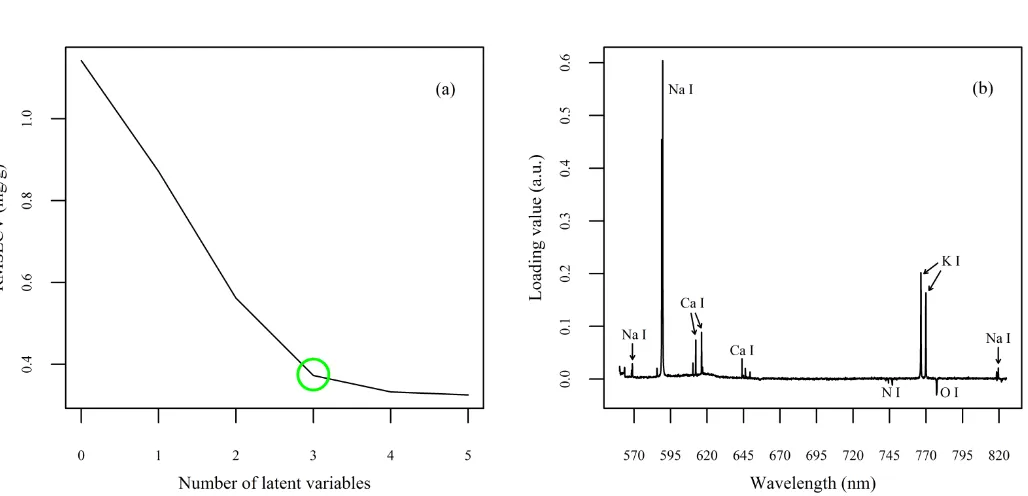
The hydrogen-normalised third-layer-spectra model was used as the calibration to perform 286
sodium content predictions. Fig. 2 (a) shows the values of RMSECV for each LV of this 287
model. A number of 3 LVs was selected as further factors did not result in a notable 288
improvement in terms of RMSECV while, at the same time, the quality of the predictions for 289
the validation set decreased, indicating that a higher number of LVs could result in overfitting 290
of the model. The first 3 main LVs explained approximately 95.7% of the total spectral 291
variance. 292
Fig. 2 (b) shows the loading values for the first factor of the PLS model in the wavelength 293
range assessed. One main sodium (Na I) emission line at 589.59 nm contributed to the 294
loading values. Other Na I spectral lines were the doublet at 568.26 and 568.82 nm, and the 295
emission line at 819.48 nm. These spectral lines had a relatively small contribution as 296
compared to the sodium doublet at around 589 nm. Negative loading values were only 297
observed for nitrogen (N I 744.23 and 746.83 nm) and oxygen (O I 777.19 nm), both 298
elements showing minor values. 299
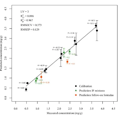
The PLS model exhibited an R2 of 0.93 for the calibration. With regards to cross-validation, 300
an R2CV value of 0.886 and an RMSECV of 0.373 mg/g were obtained, indicating a reasonable 301
fit and accuracy of the calibration. The validation of the PLS model was carried out by 302
predicting the Na contents of 2 samples not included in the training set with the aim of 303
evaluating the robustness of the model. The model exhibited a good prediction accuracy as 304
indicated by a high R2p (coefficient of determination for the validation set) of 0.967 and a 305
RMSEP value of 0.129 mg Na/g. Fig. 3 shows the PLS calibration curve with the predicted 306
values for the validation set. To further evaluate the closeness of the predictions to the actual 307
values of concentration, the relative error (RE) was calculated as reported elsewhere (Câmara 308
14
Additionally, Na contents for 2 follow-on formulas were also predicted in order to explore 310
the model’s response to different formulations of infant products. In this case, the predictions 311
were not as accurate as the validation set, giving a RE value of 23.32%. However, this result 312
may indicate that the model can provide reasonable predictions even with a certain degree of 313
variability in the raw materials. 314
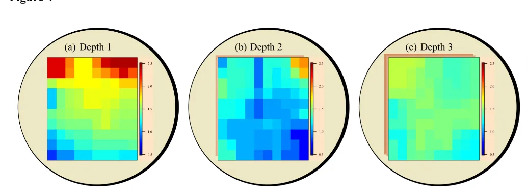
As mentioned before , the best performance was given by spectra collected after 3 laser shots. 315
To further investigate why the third layer provided better results, sodium content was 316
predicted, in this case, for each location in the 10×10 measuring grid. In order to do so, the 317
raw spectral data acquired from sample V2, chosen as a point close to the centre of the 318
calibration curve, was normalised by the hydrogen emission line without averaging the data 319
of multiple locations, i.e. obtaining 500 pre-processed spectra instead of 5. Na contents were 320
subsequently predicted employing the coefficients extracted from the PLS model. Fig. 4 321
shows a schematic representation of the V2 pellet displaying sodium content in each spatial 322
position for the first 3 measurement depths. The same intensity scale for the three 323
measurements was implemented to allow comparison. It can be observed that the predictions 324
for the third layer, Fig.4(c), provided a more homogeneously distributed sodium within the 325
analysed area. 326
The limit of detection of the model was estimated by following the pseudounivariate 327
approach as described in Eq. 2. The LOD value corresponding to the calibration model was 328
1.11 mg/g. 329
4.Conclusions 330
LIBS was successfully applied for quantifying sodium over a range in conformity with the 331
product’s regulatory guidelines, hence, demonstrating the feasibility of the technique as a 332
potential screening tool for IF manufacturing. Multivariate analysis with PLS was applied to 333
15
and accumulations. The resulting calibration models were compared in terms of PLS 335
performance: coefficients of determination and root-mean-square errors; for calibration (R2, 336
RMSEC), leave-one-out cross-validation (R2CV, RMSECV) and validation (R2p, RMSEP). The 337
best PLS calibration was obtained using the third-layer spectra normalised by the H I 338
emission line at 656.29 nm, yielding a R2 of 0.93 and a R2CV of 0.886. When performing 339
validation of this model, the resulting R2p and RMSEP values were 0.967 and 0.129 mg Na/g 340
respectively, proving its ability to accurately predict samples not included in the calibration 341
set. 342
In this study, accumulation of the spectra on the same spot did not notably improve the 343
performances of the PLS models as compared to using the third layer alone. Furthermore, 344
chemical mapping with PLS of the analysed area (100 measurements in a 10×10 grid pattern) 345
showed that sodium was more homogeneously distributed than for the first two layers. These 346
results suggested that conditioning the surface of the pelletized sample, while keeping a low 347
number of shots on the same spot, can provide a good predictive accuracy without the need of 348
large sampling numbers. 349
Acknowledgements 350
Funding: The authors would like to acknowledge funding from the Food Institutional 351
Research Measure, administered by the Department of Agriculture, Food and the Marine of 352
Ireland (Grant agreement: 14/F/866). 353
References 354
Abdi, H. (2010). Partial least squares regression and projection on latent structure regression 355
(PLS Regression). Wiley Interdisciplinary Reviews: Computational Statistics, 2(1), 97– 356
106. http://doi.org/10.1002/wics.51 357
Allegrini, F., & Olivieri, A. C. (2014). IUPAC-Consistent Approach to the Limit of Detection 358
16 http://doi.org/10.1021/ac501786u
360
Andersen, M.-B. S., Frydenvang, J., Henckel, P., & Rinnan, Å. (2016). The potential of laser-361
induced breakdown spectroscopy for industrial at-line monitoring of calcium content in 362
comminuted poultry meat. Food Control, 64, 226–233. 363
http://doi.org/10.1016/j.foodcont.2016.01.001 364
Bilge, G., Sezer, B., Eseller, K. E., Berberoglu, H., Topcu, A., & Boyaci, I. H. (2016). 365
Determination of whey adulteration in milk powder by using laser induced breakdown 366
spectroscopy. Food Chemistry, 212, 183–188. 367
http://doi.org/10.1016/j.foodchem.2016.05.169 368
Blanchard, E., Zhu, P., & Schuck, P. (2013). Infant formula powders. In B. Bhandari, N. 369
Bansal, M. Zhang, & P. Schuck (Eds.), Handbook of Food Powders (pp. 465–483). 370
Cambridge, UK: Woodhead Publishing. http://doi.org/10.1533/9780857098672.3.465 371
Cama-Moncunill, R., Casado-Gavalda, M. P., Cama-Moncunill, X., Markiewicz-Keszycka, 372
M., Dixit, Y., Cullen, P. J., & Sullivan, C. (2017). Quantification of trace metals in 373
infant formula premixes using laser-induced breakdown spectroscopy. Spectrochimica
374
Acta Part B: Atomic Spectroscopy, 135, 6–14. http://doi.org/10.1016/j.sab.2017.06.014 375
Cama-Moncunill, X., Markiewicz-Keszycka, M., Dixit, Y., Cama-Moncunill, R., Casado-376
Gavalda, M. P., Cullen, P. J., & Sullivan, C. (2017). Feasibility of laser-induced 377
breakdown spectroscopy (LIBS) as an at-line validation tool for calcium determination 378
in infant formula. Food Control, 78, 304–310. 379
http://doi.org/10.1016/j.foodcont.2017.03.005 380
Câmara, A. B. F., de Carvalho, L. S., de Morais, C. L. M., de Lima, L. A. S., de Araújo, H. 381
O. M., de Oliveira, F. M., & de Lima, K. M. G. (2017). MCR-ALS and PLS coupled to 382
NIR/MIR spectroscopies for quantification and identification of adulterant in biodiesel-383
17
Campbell, K. J., Hendrie, G., Nowson, C., Grimes, C. A., Riley, M., Lioret, S., & 385
McNaughton, S. A. (2014). Sources and Correlates of Sodium Consumption in the First 386
2 Years of Life. Journal of the Academy of Nutrition and Dietetics, 114(10), 1525– 387
1532.e2. http://doi.org/10.1016/j.jand.2014.04.028 388
Codex. (2007). Standard for infant formula and formulas for special medical purposes
389
intended for infants, CODEX STAN 72 – 1981. Rome, Italy: FAO/WHO Codex
390
Alimentarius. 391
Cremers, D. A., & Radziemski, L. J. (2013). Handbook of Laser-Induced Breakdown
392
Spectroscopy (2nd ed.). Chichester, UK: John Wiley & Sons Ltd. 393
Cullen, P., Bakalis, S., & Sullivan, C. (2017). Advances in control of food mixing operations. 394
Current Opinion in Food Science, 17(Supplement C), 89–93.
395
http://doi.org/https://doi.org/10.1016/j.cofs.2017.11.002 396
Dixit, Y., Casado-Gavalda, M. P., Cama-Moncunill, R., Cama-Moncunill, X., Markiewicz-397
Keszycka, M., Jacoby, F., … Sullivan, C. (2017). Introduction to laser induced 398
breakdown spectroscopy imaging in food: Salt diffusion in meat. Journal of Food
399
Engineering. http://doi.org/10.1016/j.jfoodeng.2017.08.010 400
dos Santos Augusto, A., Barsanelli, P. L., Pereira, F. M. V., & Pereira-Filho, E. R. (2017). 401
Calibration strategies for the direct determination of Ca, K, and Mg in commercial 402
samples of powdered milk and solid dietary supplements using laser-induced breakdown 403
spectroscopy (LIBS). Food Research International. 404
http://doi.org/10.1016/j.foodres.2017.01.027 405
El Haddad, J., Canioni, L., & Bousquet, B. (2014). Good practices in LIBS analysis: Review 406
and advices. Spectrochimica Acta Part B: Atomic Spectroscopy, 101, 171–182. 407
http://doi.org/10.1016/j.sab.2014.08.039 408
18
Martin-Neto, L. (2010). Determination of Ca in breakfast cereals by laser induced 410
breakdown spectroscopy. Food Control, 21(10), 1327–1330. 411
http://doi.org/10.1016/j.foodcont.2010.04.004 412
Guo, M. (2014). 2 – Chemical composition of human milk. In M. Guo (Ed.), Human Milk
413
Biochemistry and Infant Formula Manufacturing Technology (pp. 19–32). Cambridge,
414
UK: Woodhead Publishing. http://doi.org/10.1533/9780857099150.1.19 415
Jantzi, S. C., Motto-Ros, V., Trichard, F., Markushin, Y., Melikechi, N., & De Giacomo, A. 416
(2016). Sample treatment and preparation for laser-induced breakdown spectroscopy. 417
Spectrochimica Acta Part B: Atomic Spectroscopy, 115, 52–63. 418
http://doi.org/10.1016/j.sab.2015.11.002 419
Jiang, Y. J. (2014). 11 – Infant formula product regulation. In M. Guo (Ed.), Human Milk
420
Biochemistry and Infant Formula Manufacturing Technology (pp. 273–310).
421
Cambridge, UK: Woodhead Publishing. http://doi.org/10.1533/9780857099150.3.273 422
John, K. A., Cogswell, M. E., Zhao, L., Maalouf, J., Gunn, J. P., & Merritt, R. K. (2016). US 423
consumer attitudes toward sodium in baby and toddler foods. Appetite, 103, 171–175. 424
http://doi.org/10.1016/J.APPET.2016.04.009 425
Kim, G., Kwak, J., Choi, J., & Park, K. (2012). Detection of Nutrient Elements and 426
Contamination by Pesticides in Spinach and Rice Samples Using Laser-Induced 427
Breakdown Spectroscopy (LIBS). Journal of Agricultural and Food Chemistry, 60(3), 428
718–724. http://doi.org/10.1021/jf203518f 429
Kramida, A., Ralchenko, Y., Reader, J., & NIST ASD team. (2016). NIST Atomic Spectra 430
Database (version 5.4). Retrieved December 4, 2017, from 431
https://www.nist.gov/pml/atomic-spectra-database 432
Lei, W. Q., El Haddad, J., Motto-Ros, V., Gilon-Delepine, N., Stankova, A., Ma, Q. L., … 433
19
laser-induced breakdown spectroscopy and inductively coupled plasma atomic emission 435
spectroscopy. Analytical and Bioanalytical Chemistry, 400(10), 3303–3313. 436
http://doi.org/10.1007/s00216-011-4813-x 437
Markiewicz-Keszycka, M., Moncunill, X., Casado-Gavalda, M. P., Dixit, Y., Cama-438
Moncunill, R., Cullen, P. J., & Sullivan, C. (2017). Laser-induced breakdown 439
spectroscopy (LIBS) for food analysis: A review. Trends in Food Science &
440
Technology, 65, 80–93. http://doi.org/10.1016/j.tifs.2017.05.005 441
Markiewicz-Keszycka, M., Casado-Gavalda, M. P., Cama-Moncunill, X., Cama-Moncunill, 442
R., Dixit, Y., Cullen, P. J., & Sullivan, C. (2018). Laser-induced breakdown 443
spectroscopy (LIBS) for rapid analysis of ash, potassium and magnesium in gluten free 444
flours. Food Chemistry, 244. http://doi.org/10.1016/j.foodchem.2017.10.063 445
Masotti, F., Erba, D., De Noni, I., & Pellegrino, L. (2012). Rapid determination of sodium in 446
milk and milk products by capillary zone electrophoresis. Journal of Dairy Science, 447
95(6), 2872–2881. http://doi.org/10.3168/JDS.2011-5146 448
Mevik, B.-H., Wehrens, R., & Liland, K. H. (2015). Pls: Partial Least Squares and Principal
449
Component Regression. Retrieved from
https://cran.r-450
project.org/web/packages/pls/index.html 451
Misra, N. N., Sullivan, C., & Cullen, P. J. (2015). Process Analytical Technology (PAT) and 452
Multivariate Methods for Downstream Processes. Current Biochemical Engineering, 453
2(1), 4–16. http://doi.org/10.2174/2213385203666150219231836 454
Moncayo, S., Manzoor, S., Rosales, J. D., Anzano, J., & Caceres, J. O. (2017). Qualitative 455
and quantitative analysis of milk for the detection of adulteration by Laser Induced 456
Breakdown Spectroscopy (LIBS). Food Chemistry, 232, 322–328. 457
http://doi.org/10.1016/j.foodchem.2017.04.017 458
20
Formulae – Powders and Liquids. In A. Y. Tamime (Ed.), Dairy Powders and
460
Concentrated Products (pp. 294–331). Oxford, UK: Blackwell Publishing.
461
Poitevin, E. (2016). Official Methods for the Determination of Minerals and Trace Elements 462
in Infant Formula and Milk Products: A Review. Journal of AOAC International. 463
Retrieved from 464
http://www.ingentaconnect.com/content/aoac/jaoac/2016/00000099/00000001/art00009 465
R Core Team. (2014). R: A language and environment for statistical computing. Viena, 466
Austria. Retrieved from http://www.r-poject.org/ 467
Sezer, B., Bilge, G., & Boyaci, I. H. (2017). Capabilities and limitations of LIBS in food 468
analysis. TrAC Trends in Analytical Chemistry, 97(Supplement C), 345–353. 469
http://doi.org/https://doi.org/10.1016/j.trac.2017.10.003 470
Sobron, P., Wang, A., & Sobron, F. (2012). Extraction of compositional and hydration 471
information of sulfates from laser-induced plasma spectra recorded under Mars 472
atmospheric conditions — Implications for ChemCam investigations on Curiosity rover. 473
Spectrochimica Acta Part B: Atomic Spectroscopy, 68, 1–16. 474
http://doi.org/https://doi.org/10.1016/j.sab.2012.01.002 475
Tamm, A., Bolumar, T., Bajovic, B., & Toepfl, S. (2016). Salt (NaCl) reduction in cooked 476
ham by a combined approach of high pressure treatment and the salt replacer KCl. 477
Innovative Food Science & Emerging Technologies, 36(Supplement C), 294–302. 478
http://doi.org/https://doi.org/10.1016/j.ifset.2016.07.010 479
Tognoni, E., & Cristoforetti, G. (2016). Signal and noise in Laser Induced Breakdown 480
Spectroscopy: An introductory review. Optics & Laser Technology, 79, 164–172. 481
http://doi.org/10.1016/j.optlastec.2015.12.010 482
van den Berg, F., Lyndgaard, C. B., Sørensen, K. M., & Engelsen, S. B. (2013). Process 483
21
31(1), 27–35. http://doi.org/10.1016/j.tifs.2012.04.007 485
Wu, D., & Sun, D.-W. (2013). Advanced applications of hyperspectral imaging technology 486
for food quality and safety analysis and assessment: A review — Part I: Fundamentals. 487
Innovative Food Science & Emerging Technologies, 19, 1–14. 488
http://doi.org/10.1016/J.IFSET.2013.04.014 489
22 Table 1
491
Sodium contents in milligrams per gram of samples corresponding to calibration (C1–C5) 492
and validation (V1–V4) determined by AAS. 493
Sample Constituents Batch 1 Batch 2 Extra validation Na content (mg/g) a Na content (mg/g) a Na content (mg/g) a
C1 IF + lactose 0.48 ± 0.05 0.54 ± 0.03 ‒
C2 IF 1.40 ± 0.21 1.34 ± 0.07 ‒
C3 IF + NaCl 2.11 ± 0.11 2.07 ± 0.02 ‒
C4 IF + NaCl 2.78 ± 0.16 2.72 ± 0.07 ‒
C5 IF + NaCl 3.69 ± 0.54 3.74 ± 0.18 ‒
V1 IF + lactose 0.93 ± 0.06 0.98 ± 0.06 ‒
V2 IF + NaCl 2.22 ± 0.04 2.48 ± 0.21 ‒
V3 follow-on ‒ ‒ 1.18 ± 0.04
V4 follow-on ‒ ‒ 2.38 ± 0.36
23 Table 2
495
Summary of performances for the PLS models developed using different sampling methods 496
and pre-processing techniques. 497
a Number of conditioning shots. 498
b Number of accumulated spectra. 499
Experiment Depth Pre-processing
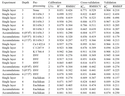
Calibration Cross-validation Validation LVs R2 RMSEC
R2CV RMSECV R 2
p RMSEP
Single layer 3 None 3 0.851 0.426 0.771 0.529 0.904 0.218 Single layer 1 H I 656.3 3 0.899 0.352 0.822 0.465 0.612 0.438 Single layer 2 H I 656.3 3 0.856 0.419 0.776 0.523 0.498 0.498 Single layer 3 H I 656.3 3 0.930 0.291 0.886 0.373 0.967 0.129 Single layer 4 H I 656.3 3 0.879 0.384 0.786 0.511 0.915 0.205 Single layer 5 H I 656.3 3 0.824 0.463 0.665 0.639 0.914 0.207 Accumulations 4 (0a/4b) H I 656.3 3 0.931 0.290 0.884 0.377 0.914 0.206
Accumulations 5(0a/5b) H I 656.3 3 0.916 0.320 0.856 0.419 0.935 0.179
Accumulations 4 (1a/3b) H I 656.3 3 0.924 0.287 0.872 0.366 0.940 0.213
Single layer 3 Ca I 422.6 3 0.937 0.276 0.893 0.361 0.966 0.131 Single layer 3 C I 247.9 3 0.923 0.306 0.876 0.389 0.894 0.229 Single layer 3 K I 766.4 3 0.942 0.266 0.911 0.330 0.908 0.213 Single layer 3 SNV 3 0.938 0.276 0.888 0.369 0.945 0.164 Single layer 4 SNV 3 0.917 0.318 0.851 0.426 0.866 0.258 Single layer 5 SNV 2 0.865 0.405 0.816 0.473 0.911 0.210 Accumulations 4 (0a/4b) SNV 2 0.879 0.384 0.840 0.442 0.849 0.274
Accumulations 5(0a/5b) SNV 2 0.881 0.382 0.841 0.441 0.897 0.225
Accumulations 4 (1a/3b) SNV 2 0.878 0.389 0.831 0.446 0.888 0.312
[image:23.595.65.548.155.526.2]24 Figure 1
500
Fig. 1. Averaged spectra corresponding to, from top to bottom, the sodium chloride -IF mixture 501
at approx. 3.7 mg Na/g, the pure IF sample at approx. 1.3 mg Na/g and the sodium lactose-IF 502
25 Figure 2
504
Fig. 2. (a) RMSECV (root-mean-square error of cross-validation) for each number of PLS 505
26 Figure 3
[image:26.595.79.458.99.467.2]507
Fig. 3. PLS calibration model developed using the third-layer spectra and normalised by the 508
H I 656.29 emission line showing predicted Na contents for the validation and follow-on 509
27 Figure 4
511
Fig.4. Predictedsodium maps for the validation sample at 2.48 mg/g of sodium for the first 512
three depths: (a) first layer, (b) second layer, (c) third layer. The same intensity scale was 513