Probability density function estimation using orthogonal forward regression

Probability Density Function Estimation Using

Orthogonal Forward Regression

S. Chen, X. Hong and C.J. Harris

Abstract— Using the classical Parzen window estimate as the target function, the kernel density estimation is formulated as a regression problem and the orthogonal forward regression tech-nique is adopted to construct sparse kernel density estimates. The proposed algorithm incrementally minimises a leave-one-out test error score to select a sparse kernel model, and a local regularisation method is incorporated into the density construction process to further enforce sparsity. The kernel weights are finally updated using the multiplicative nonnegative quadratic programming algorithm, which has the ability to reduce the model size further. Except for the kernel width, the proposed algorithm has no other parameters that need tuning, and the user is not required to specify any additional criterion to terminate the density construction procedure. Two examples are used to demonstrate the ability of this regression-based approach to effectively construct a sparse kernel density estimate with comparable accuracy to that of the full-sample optimised Parzen window density estimate.

I. INTRODUCTION

An effective method of estimating the probability density function (PDF) based on a realisation sample drawn from the underlying density is based on a non-parametric approach [1]-[3]. The Parzen window (PW) estimate [1] is a remark-ably simple and accurate non-parametric density estimation technique. Because the PW estimate, also known as the kernel density estimate, employs the full data sample set in defining density estimate for subsequent observation, its computational cost for testing scales directly with the sample size, and this imposes a practical difficulty in employing the PW estimator. It also motivates the research on the so-called sparse kernel density estimation techniques. The support vector machine (SVM) method has been proposed as a promising tool for sparse kernel density estimation [4]-[6]. An interesting sparse kernel density estimation technique is proposed in [7]. Similar to the SVM methods, this technique employs the full data sample set as the kernel set and tries to make as many kernel weights to (near) zero as possible, and thus to obtain a sparse representation. The difference with the SVM approach is that it adopts the criterion of the integrated squared error between the unknown underlying density and the kernel density estimate, calculated on the training sample set.

A regression-based sparse kernel density estimation method was reported in [8]. By converting the kernels into the associated cumulative distribution functions and using

S. Chen and C.J. Harris are with School of Electronics and Computer Science, University of Southampton, Southampton SO17 1BJ, UK, E-mails: {sqc,cjh}@ecs.soton.ac.uk

X. Hong is with School of Systems Engineering, University of Reading, Reading RG6 6AY, UK, E-mail: x.hong@reading.ac.uk

the empirical distribution function as the desired respone, just like the SVM-based density estimation [4]-[6], this technique transfers the kernel density estimation into a regression problem and it selects sparse kernel density estimates based on an orthogonal forward regression (OFR) algorithm that incrementally minimises the training mean square error (MSE). An additional termination criterion based on the minimum descriptive length [9] or Akaike’s information criterion [10] is adopted to stop the kernel density construc-tion procedure. Motivated by our previous work on sparse regression modelling [11],[12], recently we have proposed an efficient construction algorithm for sparse kernel density estimation using the OFR based on the leave-one-out (LOO) MSE and local regularisation [13]. This method is capable of constructing very sparse kernel density estimates with comparable accuracy to that of the full-sample optimised PW density estimate. Moreover, the process is fully automatic and the user is not required to specify when to terminate the density construction procedure [13].

In the works [8],[13], the “regressors” are the cumulative distribution functions of the corresponding kernels and the target function is the empirical distribution function calcu-lated on the training data set. Computing the cumulative dis-tribution functions can be inconvenient and may be difficult for certain types of kernels. We propose a simple regression-based alternative, which directly uses the PW estimate as the desired response. The same OFR algorithm based on the LOO MSE and local regularisation [12] can readily be employed to select a sparse model. Unlike the work [13], we use the multiplicative nonnegative quadratic programming (MNQP) algorithm [14] to compute the final weights of the kernel density estimate, which has a desired property of driv-ing many kernel weights to (near) zero and thus is capable of further reducing the model size. Our empirical results show that this method offers a viable simple alternative to the regression-based sparse kernel density estimation.

II. REGRESSION-BASEDAPPROACH FORKERNEL

DENSITYESTIMATION

Based on a data sample set _D={xk}Nk=1 drawn from a

density p(x), where xk ∈ Rm, the task is to estimate the

unknown densityp(x)using the kernel density estimate

ˆ

p(x;β, ρ) =

N

X

k=1

βkKρ(x,xk) (1)

with the constraints

βk≥0, 1≤k≤N, (2)

1-4244-1380-X/07/$25.00 ©2007 IEEE

and

βT1= 1, (3)

where β = [β1 β2· · ·βN]T is the kernel weight vector, 1

denotes the vector of ones with an appropriate dimension, and Kρ(•,•) is a chosen kernel function with the kernel

width ρ. In this study, we use the Gaussian kernel of the form

Kρ(x,xk) = 1

(2πρ2₎m/2e

−kx−xkk2

2ρ2 . ₍₄₎

Many other types of kernel functions can also be used in the density estimate (1).

The well-known PW estimatepˆ(x;βPar, ρPar)is obtained

by setting all the elements of βPar to N1. The optimal

kernel widthρParis typically determined via cross validation [15],[16]. The PW estimate in fact can be derived as the maximum likelihood estimator using the divergence-based criterion [17]. The negative cross-entropy or divergence between the true density p(x) and the estimate pˆ(x;β, ρ) is defined as

Z

Rm

p(u) log ˆp(u;β, ρ)du≈ _N1

N

X

k=1

log ˆp(xk;β, ρ)

= 1

N N

X

k=1

log

N

X

n=1

βnKρ(xk,xn)

!

. (5)

Minimising this divergence subject to the constraints (2) and (3) leads to βn = _N1 for1≤n≤N, i.e. the PW estimate.

Because of this property, we can view the PW estimate as the “observation” of the true density contaminated by some “observation noise”, namely

ˆ

p(x;βPar, ρPar) =p(x) + ˜ǫ(x). (6)

Thus the generic kernel density estimation problem (1) can be viewed as the following regression problem with the PW estimate as the desired response

ˆ

p(x;β_Par, ρPar) =

N

X

k=1

βkKρ(x,xk) +ǫ(x) (7)

subject to the constraints (2) and (3), where ǫ(x) is the modelling error atx. Defineyk= ˆp(xk;βPar, ρPar),φ(k) =

[Kk,1 Kk,2· · ·Kk,N]T withKk,i=Kρ(xk,xi), andǫ(k) = ǫ(xk). Then the model (7) at the data pointxk ∈ D can be

expressed as

yk = ˆyk+ǫ(k) =φT(k)β+ǫ(k). (8)

The model (8) is a standard regression model, and over the training data set _Dit can be written in the matrix form

y=Φβ+ǫ (9)

with the following additional notations Φ = [Ki,k] ∈

RN×N_{, 1 ≤ i, k ≤ N, ǫ = [ǫ(1) ǫ(2)· · ·ǫ(N)]}T_{, and} y = [y1 y2· · ·yN]T. For convenience, we will denote

the regression matrix Φ = [φ1 φ2· · ·φN] with φk =

[K1,k K2,k· · ·KN,k]T. Note that φk is thekth column of Φ, whileφT(k)is thekth row ofΦ.

Let an orthogonal decomposition of the regression matrix

Φ be Φ = WA, where W = [w1 w2· · ·wN] with

orthogonal columns satisfyingwT_i wj= 0, ifi6=j, and

A=



    

1 a1,2 · · · a1,N

0 1 . .. ... ..

. . .. . .. aN−1,N

0 · · · 0 1



    

. (10)

The regression model (9) can alternatively be expressed as

y=Wg+ǫ (11)

where the weight vector g = [g1 g2· · ·gN]T defined in

the orthogonal model space satisfies Aβ = g. The space spanned by the original model bases φi, 1 ≤ i ≤ N, is

identical to the space spanned by the orthogonal model bases

wi,1≤i≤N, and the modelyˆk is equivalently expressed

by

ˆ

yk=wT(k)g (12)

wherewT_{(k) = [w}

k,1 wk,2· · ·wk,N]is thekth row ofW.

III. ORTHOGONALFORWARDREGRESSION FORSPARSE

DENSITYESTIMATION

Our aim is to seek a sparse representation forpˆ(x;β, ρ) and yet maintaining a comparable test performance to that of the PW estimate. Since this density construction problem is formulated as a standard regression problem, the OFR algorithm based on the LOO MSE and local regularisation [12] can readily be applied to select a sparse model represen-tation. For the completeness, this OFR-LOO-LR algorithm is summarised.

The local regularisation aided least squares solution for the weight parameter vectorgis obtained by minimising the regularised error criterion [18]

JR(g,λ) =ǫTǫ+ N

X

i=1

λig2i (13)

where λ = [λ1 λ2· · ·λN]T is the regularisation parameter

vector, which is optimised based on the evidence procedure [19] with the iterative updating formulas [11],[12],[18]

λnewi = γold

i N−γold

ǫT_ǫ g2

i

, 1≤i≤N, (14)

where

γi=

wT_i wi λi+wTi wi

and γ=

N

X

i=1

γi. (15)

Typically a few iterations are sufficient to find a (near) opti-malλ. The use of multiple-regularisers or local regularisation is capable of providing very sparse solutions [18],[20].

is a measure of the model’s generalisation performance [16],[21]-[23]. At the nth stage of the OFR procedure, an

n-term model is selected. It can be shown that the LOO test error, denoted as ǫn,−k(k), for the selectedn-term model is

[12],[23]

ǫn,−k(k) = ǫn(k) ηn(k)

(16)

whereǫn(k)is then-term modelling error and ηn(k) is the

associated LOO error weighting. The LOO MSE for the model with a size nis defined by

Jn=

1

N N

X

k=1

ǫ2n,−k(k) =

1

N N

X

k=1 ǫ2

n(k) η2

n(k)

. (17)

Jncan be computed efficiently due to the fact that then-term

model error ǫn(k) and the associated LOO error weighting ηn(k)can be calculated recursively according to [12],[23]

ǫn(k) =ǫn−1(k)−wk,ngn (18)

and

ηn(k) =ηn−1(k)− w2

k,n wT

nwn+λn

. (19)

The subset model selection procedure is carried as follows: at the nth stage of the selection procedure, a model term is selected among the remaining n to N candidates if the resultingn-term model produces the smallest LOO MSEJn.

The selection procedure is terminated when

Jns+1≥Jns, (20)

yielding a ns-term sparse model. It is known that Jn is

at least locally convex with respect to the model size n

[23]. That is, there exists an “optimal” model size ns such

that for n ≤ ns Jn decreases as n increases while the

condition (20) holds. This property enables the selection procedure to be automatically terminated with an ns-term

model, without the need for the user to specify a separate termination criterion. The sparse model selection procedure is summarised as follows.

Initialisation: Set allλito10−6and iteration index toI= 1. Step 1: Given the currentλand the initial conditions

ǫ0(k) =yk and η0(k) = 1, 1≤k≤N, J0= _N1yTy= _N1 PN

k=1y2k,

(21)

use the procedure described in Appendix to select a subset model with nI terms.

Step 2: Update λ using (14) and (15) with N = nI. If a

pre-set maximum iteration number (e.g. 10) is reached, stop; otherwise setI+ = 1and go to Step 1.

In the work [13], the nonnegative constraint (2) is guaran-teed by modifying the selection procedure as follows. In the

nth stage, a candidate that causes the weight vector βn to

have negative elements, if included, will not be considered at all. The unit length condition (3) is met by normalising the final ns-term model weights. We adopt an alternative

means of meeting constraints (2) and (3) by updating the weights of the sparse model using MNQP algorithm [14],

which is known to be capable of driving many kernel weights to (near) zero and thus further reducing the size of the kernel density estimate. Denote the design matrix of the selected sparse model as B = ΦT_nsΦns = [bi,j] and the vector v = ΦT_nsy = [v1· · ·vns]

T_{. The MNQP algorithm updates}

the kernel weights according to

c(_it)=β_i(t)





ns

X

j=1 bi,jβ(jt)



 −1

, 1≤i≤ns, (22)

h(t)=

ns

X

i=1 c(_it)

!−1

1−

ns

X

i=1 c(_it)vi

!

, (23)

βi(t+1)=c (t) i

vi+h(t)

, (24)

where the superindex (t) denotes the iteration index. The initial condition can be set as β_i(0)= 1

ns,1≤i≤ns.

IV. TWONUMERICALEXAMPLES

Two examples were used in the simulation to test the proposed algorithm for constructing sparse kernel density (SKD) estimate and to compare its performance with the PW estimator. The value of the kernel width ρ used was determined by test performance via cross validation. For each example, a data set ofN randomly drawn samples was used to construct kernel density estimates, and a separate test data set ofNtest= 10,000samples was used to calculate theL1

test error for the resulting estimate according to

L1= 1

Ntest Ntest

X

k=1

|p(xk)−pˆ(xk;β, ρ)|. (25)

The experiment was repeated byNrun random runs.

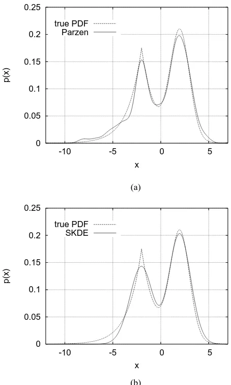
Example 1. This was a one-dimensional example, and the density to be estimated was the mixture of Gaussian and Laplacian given by

p(x) = 1 2√2πe

−(x−₂2)2 ₊0.7

4 e

−0.7|x+2|_{. (26)}

The number of data points for density estimation wasN = 100. The optimal kernel widths were found to beρ= 0.54 and ρ = 1.1 empirically for the PW estimate and the SKD estimate, respectively. The experiment was repeated

Nrun = 200 times. Table I compares the performance of

0 0.05 0.1 0.15 0.2 0.25

-10 -5 0 5

p(x)

x true PDF

Parzen

(a)

0 0.05 0.1 0.15 0.2 0.25

-10 -5 0 5

p(x)

x true PDF

SKDE

(b)

Fig. 1. (a) true density (dashed) and a Parzen window estimate (solid), and (b) true density (dashed) and a sparse kernel density estimate (solid), for the one-dimensional example of Gaussian and Laplacian mixture.

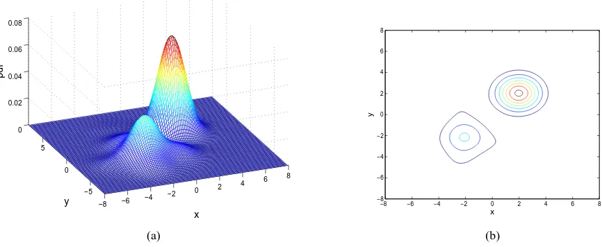
Example 2. The density to be estimated for this two-dimensional example was defined by the mixture of Gaussian and Laplacian given as follows

p(x, y) = 1 4πe

−(x−₂2)2_e−(y−₂2)2

+0.35 8 e

−0.7|x+2|_e−0.5|y+2|_{. (27)}

Fig. 2 shows this density distribution and its contour plot. The estimation data set contained N = 500 samples, and the empirically found optimal kernel widths wereρ= 0.42 for the PW estimate and ρ = 1.1 for the SKD estimate, respectively. The experiment was repeated Nrun = 100

times. Table II lists the L1 test errors and the numbers of kernels required for the two density estimates. A typical PW estimate and a typical SKD estimate are depicted in Figs. 3 and 4, respectively. Again, for this example, the two density estimates had comparable accuracies, but the SKD estimate method achieved sparse estimates with an average number of required kernels less than 4% of the data samples. The maximum and minimum numbers of kernels over 100 runs

TABLE I

PERFORMANCE OF THEPARZEN WINDOW ESTIMATE AND THE SPARSE KERNEL DENSITY ESTIMATE IN TERMS OFL1TEST ERROR AND NUMBER

OF KERNELS REQUIRED FOR THE ONE-DIMENSIONAL EXAMPLE OF GAUSSIAN ANDLAPLACIAN MIXTURE,QUOTED AS MEAN±STANDARD

DEVIATION OVER200RUNS.

method L1test error kernel number

PW estimate (1.9503±0.5881)×10−2 _100±0

SKD estimate (1.9436±0.6208)×10−2 5_.1±1_.3

were 25 and 8, respectively, for the SKD estimate.

V. CONCLUSIONS

An simple kernel density estimation method has been pro-posed based on a regression approach with the Parzen win-dow estimate as the target function. The orthogonal forward regression algorithm has been employed to select sparse ker-nel density estimates, by incrementally minimising a leave-one-out mean square error coupled with local regularisation to further enforce the sparseness of density estimates. The kernel weights are then updated using the MNQP algorithm. The proposed method is simple to implement, and except for the kernel width the algorithm contains no other free parameters that require tuning. The ability of the proposed method to construct a sparse kernel density estimate with a comparable accuracy to that of the full-sample optimised Parzen window estimate has been demonstrated using two examples. The results obtained have shown that the proposed method offers a viable alternative for sparse kernel density estimation.

APPENDIX THEOFR-LOO-LR ALGORITHM

The modified Gram-Schmidt orthogonalisation procedure [24] calculates theAmatrix row by row and orthogonalises

Φas follows: at thelth stage make the columnsφ_j,l+ 1≤

j≤N, orthogonal to thelth column and repeat the operation for 1≤l ≤N−1. Specifically, denoting φ(0)_j =φ_j, 1 ≤

j≤N, then forl= 1,2,· · ·, N−1,

wl=φ(_ll−1),

al,j =wTlφ (l−1)

j / wlTwl, l+ 1≤j≤N,

φ(_jl)=φ_j(l−1)₋al,jwl, l+ 1≤j ≤N.

    

   

(28)

TABLE II

PERFORMANCE OF THEPARZEN WINDOW ESTIMATE AND THE SPARSE KERNEL DENSITY ESTIMATE IN TERMS OFL1TEST ERROR AND NUMBER

OF KERNELS REQUIRED FOR THE TWO-DIMENSIONAL EXAMPLE OF GAUSSIAN ANDLAPLACIAN MIXTURE,QUOTED AS MEAN±STANDARD

DEVIATION OVER100RUNS.

method L1test error kernel number

PW estimate (4.2453±0.8242)×10−3 500±0

The last stage of the procedure is simply wN = φ(NN−1).

The elements of gare computed by transformingy(0) =y

in a similar way

gl=wlTy(l−1)/ wTl wl+λl,

y(l)=y(l−1)₋glwl,

)

1≤l≤N. (29)

At the beginning of thelth stage of the OFR procedure, the

l−1regressors have been selected and the regression matrix can be expressed as

Φ(l−1)=hw1· · ·wl−1 φ(ll−1)· · ·φ (l−1) N

i

. (30)

Let a very small positive numberTzbe given, which specifies

the zero threshold and is used to automatically avoiding any ill-conditioning or singular problem. With the initial conditions as specified in (21), thelth stage of the selection procedure is given as follows.

Step 1. Forl≤j≤N:

• Test – Conditioning number check. If

φ(jl−1)

T

φ(jl−1) < Tz, the jth candidate is not

considered.

• Compute

g(_lj)=φ(_jl−1) T

y(l−1)/

φ(_jl−1) T

φ(_jl−1)+λj

,

ǫ_l(j)(k) =y_k(l−1)−φ(jl−1)(k)g (j) l

η_l(j)(k) =ηl−1(k)−

φ(_jl−1)(k)2 φ(l−1)

j

T φ(l−1)

j +λj

   

  

fork= 1,· · ·, N, and

J_l(j)= 1

N N

X

k=1

ǫ(_lj)(k)

η_l(j)(k)

!2

where y_k(l−1) and φ_j(l−1)(k) are the kth elements of

y(l−1) and φ(jl−1), respectively. Let the index set Jl

be

Jl={l≤j≤N andj passes Test} Step 2. Find

Jl=Jl(jl)= min{J (j)

l , j∈ Jl}

Then thejlth column ofΦ(l−1)is interchanged with thelth

column ofΦ(l−1), thejlth column ofAis interchanged with

the lth column of A up to the (l−1)th row, and the jlth

element ofλis interchanged with thelth element ofλ. This effectively selects the jlth candidate as the lth regressor in

the subset model.

Step 3. The selection procedure is terminated with a(l−1) -term model, if Jl ≥Jl−1. Otherwise, perform the

orthogo-nalisation as indicated in (28) to derive the l-th row of A

and to transform Φ(l−1) into Φ(l); calculate gl and update y(l−1) _{into y}(l) _{in the way shown in (29); update the LOO}

error weightings

ηl(k) =ηl−1(k)−

w2k,l wT

lwl+λl

, k= 1,2,· · ·, N

and go to Step 1.

REFERENCES

[1] E. Parzen, “On estimation of a probability density function and mode,”

The Annals of Mathematical Statistics, vol.33, pp.1066–1076, 1962.

[2] C.M. Bishop, Neural Networks for Pattern Recognition. Oxford, U.K.: Oxford University Press, 1995.

[3] B.W. Silverman, Density Estimation. London: Chapman Hall, 1996. [4] J. Weston, A. Gammerman. M.O. Stitson, V. Vapnik, V. Vovk and

C. Watkins, “Support vector density estimation,” in: B. Sch¨olkopf, C. Burges and A.J. Smola, eds., Advances in Kernel Methods — Support

Vector Learning, MIT Press, Cambridge MA, 1999, pp.293–306.

[5] S. Mukherjee and V. Vapnik, “Support vector method for multivariate density estimation,” Technical Report, A.I. Memo No. 1653, MIT AI Lab, 1999.

[6] V. Vapnik and S. Mukherjee, “Support vector method for multivariate density estimation,” in: S. Solla, T. Leen and K.R. M¨uller, eds.,

Advances in Neural Information Processing Systems, MIT Press, 2000,

pp.659–665.

[7] M. Girolami and C. He, “Probability density estimation from optimally condensed data samples,” IEEE Trans. Pattern Analysis and Machine

Intelligence, vol.25, no.10, pp.1253–1264, 2003.

[8] A. Choudhury, Fast Machine Learning Algorithms for Large Data. PhD Thesis, Computational Engineering and Design Center, School of Engineering Sciences, University of Southampton, 2002. [9] M.H. Hansen and B. Yu, “Model selection and the principle of

minimum description length,” J. American Statistical Association, vol.96, no.454, pp.746–774, 2001.

[10] H. Akaike, “A new look at the statistical model identification,” IEEE

Trans. Automatic Control, vol.AC-19, pp.716–723, 1974.

[11] S. Chen, X. Hong and C.J. Harris, “Sparse kernel regression modeling using combined locally regularized orthogonal least squares and D-optimality experimental design,” IEEE Trans. Automatic Control, vol.48, no.6, pp.1029–1036, 2003.

[12] S. Chen, X. Hong, C.J. Harris and P.M. Sharkey, “Sparse modeling using orthogonal forward regression with PRESS statistic and regular-ization,” IEEE Trans. Systems, Man and Cybernetics, Part B, vol.34, no.2, pp.898–911, 2004.

[13] S. Chen, X. Hong and C.J. Harris, “Sparse kernel density construction using orthogonal forward regression with leave-one-out test score and local regularization,” IEEE Trans. Systems, Man and Cybernetics, Part

B, vol.34, no.4, pp.1708–1717, 2004.

[14] F. Sha, L.K. Saul and D.D. Lee, “Multiplicative updates for nonneg-ative quadratic programming in support vector machines,” Technical

Report. MS-CIS-02-19, University of Pennsylvania, USA, 2002.

[15] M. Stone, “Cross validation choice and assessment of statistical predictions,” J. Royal Statistics Society Series B, vol.36, pp.111–147, 1974.

[16] R.H. Myers, Classical and Modern Regression with Applications. 2nd Edition, Boston: PWS-KENT, 1990.

[17] G. McLachlan and D. Peel, Finite Mixture Models. John Wiley, 2000. [18] S. Chen, “Local regularization assisted orthogonal least squares

re-gression,” Neurocomputing, vol.69, no.4-6, pp.559–585, 2006. [19] D.J.C. MacKay, “Bayesian interpolation,” Neural Computation, vol.4,

no.3, pp.415–447, 1992.

[20] M.E. Tipping, “Sparse Bayesian learning and the relevance vector machine,” J. Machine Learning Research, vol.1, pp.211–244, 2001. [21] L.K. Hansen and J. Larsen, “Linear unlearning for cross-validation,”

Advances in Computational Mathematics, vol.5, pp.269–280, 1996.

[22] G. Monari and G. Dreyfus, “Local overfitting control via leverages,”

Neural Computation, vol.14, pp.1481–1506, 2002.

[23] X. Hong, P.M. Sharkey and K. Warwick, “Automatic nonlinear pre-dictive model construction algorithm using forward regression and the PRESS statistic,” IEE Proc. Control Theory and Applications, vol.150, no.3, pp.245–254, 2003.

[24] S. Chen, S.A. Billings and W. Luo, “Orthogonal least squares meth-ods and their application to non-linear system identification,” Int. J.

−8 −6

−4 −2 0

2 4

6 8

−5 0 5 0 0.02 0.04 0.06 0.08

x y

pdf

x

y

−8 −6 −4 −2 0 2 4 6 8

−8 −6 −4 −2 0 2 4 6 8

(a) (b)

Fig. 2. True density (a) and contour plot (b) for the two-dimensional example of Gaussian and Laplacian mixture.

−8 −6 −4

−2 0

2 4 6

8

−5 0 5 0 0.02 0.04 0.06 0.08

x y

pdf

x

y

−8 −6 −4 −2 0 2 4 6 8

−8 −6 −4 −2 0 2 4 6 8

(a) (b)

Fig. 3. A Parzen window estimate (a) and contour plot (b) for the two-dimensional example of Gaussian and Laplacian mixture.

−8 −6 −4

−2 0

2 4

6 8

−5 0 5 0 0.02 0.04 0.06 0.08

x y

pdf

x

y

−8 −6 −4 −2 0 2 4 6 8

−8 −6 −4 −2 0 2 4 6 8

(a) (b)