Interactive visualisation techniques for data mining of satellite imagery

(1)

Interactive Visualisation

Techniques for Data Mining of

Satellite Imagery

By

Samuel John Welch, BComp

A dissertation submitted to the

School of Computing

In partial fulfilment of the requirements for the degree of

Bachelor of Computing with Honours

University of Tasmania

(2)

Declaration

I, Samuel John Welch declare that this thesis contains no material which has been accepted for the award of any other degree or diploma in any tertiary institution. To my knowledge and belief, this thesis contains no material previously published or written by another person except where due reference is made in the text of the thesis.

(3)

Abstract

Supervised classification of satellite imagery largely removes the user from the information extraction process. Visualisation is an often ignored means by which users may interactively explore the complex patterns and relationships in satellite imagery. Classification can be considered a “hypothesis testing” form of analysis. Visual Data Mining allows for dynamic hypothesis generation, testing and revision based on a human user’s perception. In this study Visual Data Mining was applied to the classification of satellite imagery.

After reviewing appropriate techniques and literature a tool was developed for the visual exploration and mining of satellite image data. This tool augments existing semi-automatic data mining techniques with visualisation capabilities. The tool was developed in IDL as an extension to ENVI, a popular remote sensing package.

(4)

Acknowledgements

Firstly, I would like to thank my supervisors, Dr. Ray Williams and Dr. Arko Lucieer. Ray and Arko’s feedback and guidance this year helped immensely. Arko’s work in preparing the Heard Island data for Humphrey and I was very much appreciated. Thanks go to both Arko and Ray for weathering my storm of last minute re-writes.

Thanks are due to my fellow honours room residents, Luke, Tristan, Matt, Jaidev, and Mathew, and to the rest of the Hobart honours crew. Some humour and a few games made for an enjoyable work environment. Thanks also to Humphrey in Launceston. It’s been good working with you this year and it’s been interesting to see how our two projects developed independently and yet, in the end, each has much to contribute to the other.

Many thanks are also due to my parents. Mum and Dad, your support and encouragement have been greatly appreciated.

(5)

List of Figures

FIGURE 2-1:REFLECTANCE IN EACH OF THE LANDAT TM SATELLITES 6 BANDS . ... 5

FIGURE 2-2:LANDAT TM IMAGE OF HOBART,TASMANIA IN VISIBLE LIGHT (BANDS 3,2 AND 1)... 6

FIGURE 2-3:FALSE COLOUR COMPOSITE USING BANDS 4,1 AND 5 OF THE LANDSAT TM IMAGE OF HOBART... 6

FIGURE 2-4:THEMATIC MAP OF THE LANDSAT TMHOBART IMAGE... 8

FIGURE 2-5:A SAMPLE FEATURE SPACE PLOT. ... 10

FIGURE 2-6:FEATURE SPACE PLOTS. ... 11

FIGURE 2-7:EXAMPLES OF DIFFERENT SCIENTIFIC VISUALISATIONS. ... 17

FIGURE 2-8:MRI OF THE HUMAN HEAD AND 2 SLICES EXTRACTED FROM THE VOLUME... 18

FIGURE 2-9:VOLUME RENDERING OF A CT SCAN OF AN ENGINE COMPONENT... 20

FIGURE 3-1:EXAMPLE VOLUME RENDERING SHOWING VARYING VOXEL VALUES... 26

FIGURE 3-2:RANGES OF PIXEL VALUES TO BE SORTED TO FIVE COLUMNS... 27

FIGURE 3-3:RANGES OF PIXEL VALUES TO BE SORTED TO TEN COLUMNS. ... 27

FIGURE 3-4:SCREEN CAPTURES FROM AN EXAMPLE USAGE SCENARIO.. ... 31

FIGURE 3-5:ELLIPSOIDS FOR REGIONS DEFINED IN FIGURE 3-4A AT 60% TRANSPARENCY... 32

FIGURE 3-6:Α-SHAPES FOR A SAMPLE POINT SET... 33

FIGURE 3-7:EXAMPLE FORMATION OF A 2DΑ-SHAPE... 34

FIGURE 3-8:THREE ISOSURFACES FOR A CLUSTER OF POINTS IN FEATURE SPACE... 36

FIGURE 3-9:MARCHING CUBE (LORENSEN &CLINE 1987)... 39

FIGURE 3-10:SYMMETRICALLY DISTINCT TRIANGULATIONS (LORENSEN &CLINE 1987)... 39

FIGURE 3-11:ENVI DISPLAY SHOWING ALANDSAT TM IMAGE OF HOBART,TAS. ... 41

FIGURE 3-12:FEATURE SPACE INTERSECTION WITH A VOLUME SIZE OF 64. ... 41

FIGURE 3-13:FEATURE SPACE INTERSECTION WITH A VOLUME SIZE OF 32. ... 42

FIGURE 3-14:HIGHLIGHTED CONFLICT BETWEEN REGIONS... 44

FIGURE 4-1:IMAGE BAND STATISTICS OF THE STUDY AREA... 49

FIGURE 4-2:ENVI USER INTERFACE WITH DISPLAY OF PADDICK VALLEY WITH REGIONS. ... 52

FIGURE 4-3:ISOSURFACES FOR ALL FOUR ROIS IN THE 1C-ALL ROI SET... 52

FIGURE 4-4:ISOSURFACES FOR THREE ROIS IN THE 1C-ALL ROI SET... 53

FIGURE 4-5:POTENTIAL INTERSECTION IN FEATURE SPACE BETWEEN THE ROCK AND WATER ROIS.... 53

FIGURE 4-6:ISOSURFACE REPRESENTING THE INTERSECTION BETWEEN ROCK AND WATER ROIS... 54

FIGURE 4-7:FEATURE SPACE PLOT SHOWING NO INTERSECTION BETWEEN ROIS... 54

FIGURE 4-8:OVERLAYED FALSE COLOUR COMPOSITE OF PADDICK VALLEY DEMONSTRATING HIGHLIGHTING OF CONFLICTING PIXEL VALUES. ... 55

FIGURE 4-9:PIXELS CAUSING OVERLAP... 55

FIGURE 4-10:AVERAGE SPECTRUM PLOT SHOWING HIGHER VARIANCE IN BANDS 4 AND 1. ... 56

FIGURE 4-11:INTERSECTION BETWEEN ROCK AND WATER BASED ON BANDS 4,2 AND 1.NOTE NOW THAT THE INTERSECTION FORMS TWO BLOBS IN SPACE (WHEN RENDERED AS AN ISOSURFACE) IMPLYING TWO VOXELS OF OVERLAP. ... 57

FIGURE 4-12:PIXELS CAUSING OVERLAP IN THE WATER AND ROCK REGIONS... 58

FIGURE 4-13:COMPARISON OF DECISION SURFACES. ... 59

FIGURE 4-14:MEAN POINTS FOR EACH REGION IN FEATURE... 60

FIGURE 4-15:FALSE COLOUR COMPOSITE SHOWING BANDS 4,2 AND 1 OF A SUBSET OF THE PADDICK VALLEY IMAGE... 60

FIGURE 4-16:THEMATIC IMAGE SHOWING THE RESULT OF A MINIMUM DISTANCE CLASSIFICATION OF THE IMAGE SUBSET IN FIGURE 4-15. ... 61

FIGURE 4-17:MEANS AND EXTENT FOR EACH REGION. ... 61

FIGURE 4-18:ELLIPSOIDS REPRESENTING THE DECISION BOUNDARY OF A MAXIMUM LIKELIHOOD CLASSIFIER... 62

FIGURE 4-19:THEMATIC IMAGE SHOWING THE RESULT OF A MAXIMUM LIKELIHOOD CLASSIFICATION OF THE IMAGE SUBSET IN FIGURE 4-15.. ... 63

FIGURE 4-20:COMPARISON OF Α-SHAPES AND ISOSURFACES... 64

FIGURE 4-21:THEMATIC IMAGE SHOWING THE RESULT OF A K-NEAREST NEIGHBOUR CLASSIFICATION OF THE IMAGE SUBSET IN FIGURE 4-15 ... 64

FIGURE 4-22:FEATURE SPACE PLOT SHOWING EXTENT OF REGIONS FOR A SIX VEGETATION CLASS ANALYSIS... 66

(8)

FIGURE 4-24:FALSE COLOUR COMPOSITE OF THREE DERIVED PRINCIPAL COMPONENT BANDS... 68

(9)

List of Tables

TABLE 2-1:SAMPLE FROM THE IRIS PLANTS DATABASE (FISHER 1988) ... 9

TABLE 2-2-COMMON TEXTURE MEASURES DERIVED FROM THE CO-OCCURRENCE MATRIX... 15

TABLE 4-1:MULTI-SPECTRAL WAVELENGTHS RECORDED PER BAND BY THE IKONOS SATELLITE... 47

TABLE 4-2:THE THREE CLASSIFICATION LEVELS. ... 48

TABLE 4-3:STATISTICS FOR PADDICK VALLEY IMAGE... 48

TABLE 4-4:STATISTICS FOR ORANGE REGION SHOWN IN FIGURE 4-8... 50

(10)

List of Equations

(11)

Chapter 1 Introduction

1.1 Problem Description

Satellite imagery is increasingly being used to monitor the surface of the Earth. There are numerous satellites orbiting the Earth equipped with powerful instruments for remote observation of entities and events on the ground. The data collected by these instruments is used for various purposes, such as monitoring of climate change and resource mapping. The science and art of acquiring and interpreting these images is known as remote sensing (Lillesand & Kiefer 2000; Richards 1986; Schowengerdt 1997). The extraction of spatial features is usually carried out by image interpretation and/or quantitative analysis (Richards 1986, p. 69). Image interpretation (also known as photointerpretation) requires a human analyst to visually inspect the imagery and extract information based on their experience and expert knowledge. This process can become extremely tedious due to the manner in which the data is presented and even the most expert analysts occasionally make avoidable oversights. Quantitative analysis aims to automate the interpretation stage and is generally favoured over manual image interpretation.

Classification is a quantitative analysis technique in which each pixel is assigned a thematic class based on its spectral values. This process involves statistical comparison of each pixel’s properties to that of a reference class. The problem with classification and other quantitative methods is that the user is removed from the interpretation process. This results in decreased confidence in, and understanding of, the results of such analyses (Keim, D A 2002).

(12)

1.2 Research Objectives

1.2.1 Hypothesis

It is hypothesised that combining interactive visualisation capabilities with existing techniques for data mining of remotely sensed imagery can enhance understanding of the image classification process, reveal trends in the data and produce more insightful image analyses.

1.2.2 Aim

The aim of this study is to test the hypothesis by:

• Designing and implementing a prototype visualisation system for data mining of remotely sensed imagery, and

(13)

Chapter 2 Background

2.1 Remote Sensing

2.1.1 Introduction

Remote sensing is broadly defined as the acquisition of information regarding a particular entity or event without requiring the data acquisition device to be in close proximity to the entity or event (Lillesand & Kiefer 2000). Most commonly the term refers to the use of satellite and aircraft mounted sensors for mapping and monitoring of the Earth’s surface. Numerous remote sensing satellites are orbiting the Earth. Each satellite is referred to as a platform and is home to one or more instruments or

sensors. Multiple satellites with identical sensors are sometimes referred to as a system, eg: the Landsat system (Richards 1986).

Remote sensing is more than remotely obtaining data regarding the Earth’s surface, eg: taking photographs from space. It is the science of drawing useful conclusions from the raw data, or put simply, extracting information. This process of extracting information is known as interpretation. There are two approaches to interpretation: image interpretation and quantitative analysis. These are discussed in section 2.1.4.

2.1.2 Remotely Sensed Data

(14)

Properties of remotely sensed data that are commonly discussed are its spectral, spatial and radiometric resolutions. Spectral resolution refers to the number and range of the bands in the image. Spatial resolution refers to the size, in ground units (square kilometres or metres), that each pixel represents. Finally, radiometric resolution refers to the number of discrete brightness levels available for components of each band. This is usually stated in terms of the number of binary digits used to represent the range of values.

For example, the Landsat Thematic Mapper (TM) instrument measures 61 distinct wavelength ranges; blue (0.45-0.52 µm), green (0.52-0.60 µm), and red (0.63-0.69 µm) visible light bands, a near infrared (0.76-0.90 µm) and two middle infrared (1.55-1.75 µm and 2.08-2.35 µm) bands (Richards 1986). Images from this instrument have 6 bands, one for each wavelength range. Each of these bands is recorded with a spatial resolution of 30 m; that is, each pixel represents a 30x30 m square on the ground. Each band is recorded with a radiometric resolution of 8 bits which means each element of each band can only be one of 256 discrete brightness levels.

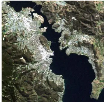
Bands for different wavelengths within an image are illustrated in Figure 2-1. The figures shown are Landsat TM images of Hobart, Tasmania, Australia acquired on 28/9/1999. Each band is displayed independently of the others in a grey scale image composition of the data for that band. The brighter any pixel in the image is, the higher its reflectance in that particular band.

1_{The Landsat Thematic Mapper does in fact have a seventh band representing thermal energy with a}

(15)

(a) (b) _(c)

[image:15.595.127.545.68.409.2]

(d) (e) (f)

Figure 2-1: Reflectance in each of the Landat TM satellites 6 bands: (a), (b), (c) Blue, green and red visible light, (d) near infrared, (e) middle infrared 1, (d) middle infrared 2.

(16)

[image:16.595.140.313.95.265.2]

Figure 2-2: Landat TM image of Hobart, Tasmania in visible light (bands 3, 2 and 1).

Figure 2-3: False colour composite using bands 4, 1 and 5 of the Landsat TM image of Hobart.

2.1.3 Pre-processing

Prior to interpretation, remotely sensed imagery is often subjected to rectification and/or enhancement. Rectification of imagery is important for obtaining accurate results. Radiometric correction is used to counter the effects of sensor noise and atmospheric refraction. Geometric correction is used rectify the geometric distortions cause by the curvature of the Earth, the angle of acquisition and topographic relied distortion. A summary of rectification techniques can be found in (Lillesand & Kiefer 2000; Richards 1986; Schowengerdt 1997). Enhancement refers to the use of image filters to stretch, smooth and sharpen imagery for visual analysis (Gonzalez & Woods 1983).

2.1.4 Interpretation

Interpretation is the key stage in the process of remote sensing. Up until this point no actual information has been gained. This section presents the two exclusive yet complementary, traditional approaches to interpretation of remotely sensed data and introduces the use of a third non-traditional approach.

(17)

expertise. This visual inspection based approach is usually quite effective in the process of segmentation. Segmentation involves extracting objects (road, buildings, lakes, rivers, etc) from the image and displaying their extent in the image. Image interpretation is not suited to the task of accurately determining the area or extent of land cover classes. Not only is it tedious for an analyst to examine every pixel in an image (as would be needed to obtain an accurate area estimate) but it is difficult for them to take into account the full reflectance profile of each pixel as only three bands are being displayed at once. Multiple false colour composites can be used to somewhat alleviate the latter issue but the problem still exists.

Whilst it is impractical for a human analyst to examine every pixel in an image, and when doing so to take into account the full dimensionality of (i.e., the number of bands in) the image the task is well suited to a computational approach. A quantitative analysis may consist of classifying each pixel in the image. Classification is a method by which labels may be attached to pixels according to their spectral characteristics (Richards 1986). This is discussed in Section 2.3. Having obtained a classification for each pixel, a colour coded thematic map of the image can be constructed (Figure 2-4). From this map the area of coverage for a given land cover class can be extracted, as well as many other measurements.

Quantitative analysis more readily yields the information that remote sensing analysts require. However, interpretation can take another key form; Visual Data Mining (VDM) or more generally scientific visualisation. This is essentially the middle ground between quantitative analysis and image interpretation. Visual data mining presents the user with a more appropriate representation of their data so that they can visually explore the relationships and patterns it contains. Like image interpretation VDM is highly subjective. This does not detract from its usefulness in remote sensing. Indeed Lillesand & Kiefer highlight the artistic nature of remote sensing:

(18)

Visualisation was used in combination with remote sensing successfully by Lucieer (2004). Visualisation and Visual Data Mining are discussed extensively in section 2.6. Its use in remote sensing is discussed in section 2.7.

(a)

(b)

Figure 2-4: (a) Thematic map of the Landsat TM Hobart image, (b) Land cover classes by colour

2.2 Data Mining

Witten & Frank (2005) define data mining as follows:

Data mining is defined as the process of discovering patterns in data. The process must be automatic or (more usually) semiautomatic. The patterns discovered must be meaningful in that they lead to some advantage, usually an economic advantage. The data is invariably present in substantial quantities.

(19)

Table 2-1: Sample from the Iris Plants Database (Fisher 1988) Instance No. Sepal Length Sepal Width Petal Length Petal Width Class

1 5.1 3.5 1.4 0.2 Iris Setosa

2 4.6 3.1 1.5 0.2 Iris Setosa

3 6.1 2.8 4.7 1.2 Iris Versicolor

4 6.3 2.9 5.6 1.8 Iris Virginica

There exist many methods for machine learning; decision trees, classification rules, artificial neural networks and instance based methods (Witten & Frank 2005). These methods all perform the operation of classification. The result of this operation is the construction of a classifier. A classifier embodies the knowledge extracted from the dataset and can be used to classify new unclassified instances. For example, if a new specimen of Iris needs to be classified, the values of the specimen’s attributes (sepal length/width, petal length/width) are given to the classifier and a class label is returned.

In the case of satellite imagery, instances are pixels. The attributes for each pixel are the bands in the image. The values are the reflectance values in each band. Class labels are assigned by an analyst to a small set of pixels in the image known as the training pixels. A classifier can be constructed and used to classify the rest of the pixels in the image.

(20)

Specific classifiers are described in section 2.3. The descriptions refer specifically to remotely sensed data rather than the general case. Many remote sensing authors tend to discuss these techniques as if they exist purely for the field of remote sensing; this of course is not true, they may be applied to virtually any classification problem.

2.2.2 Feature Space

Feature space is an abstract n-dimensional space representing the classification problem at hand. Each instance in a dataset can be plotted as a point in this space. The value of n is determined by the number of attributes in the dataset. The dimensionality can be reduced by simply ignoring certain attributes. If n is reduced to 2 or 3 the 2D or 3D feature space can be visualised.

It is useful when describing various classification algorithms to use some form of visual aid. A 3D feature space allows visualisation of the training data clusters and/or the decision boundaries used by the classifier. A 3D feature space plot can be constructed in the following manner: select three attributes from the dataset to assign to the axes of 3D Euclidean space, each instance can then be plotted according to the values of these three selected attributes. Likewise, a 2D feature space plot uses two attributes from the data set. In Figure 2-5 each instance from a sample dataset is plotted as a single point. Points are usually grouped into clusters based on class. Shapes can then be used to summarise the points in each cluster (Figure 2-6). Shapes and points allow visual explanation of classifier parameters.

(21)

(a) (b)

(c) (d)

Figure 2-6: Feature space plots; (a) Greyscale scatter plot of a 3 class dataset, (b) Ellipsoids statistically representing the 3 classes, (c) α-shapes representing the extent of classes, (d) isosurfaces representing the extent and density of classes.

2.3 Supervised Remote Sensing Image Classification

Supervised classification is the most commonly applied quantitative analysis technique for remotely sensed imagery. Image classification is the process of labelling pixels in the image as representing particular land cover types, or classes based on reference or training samples. Many algorithms exist for performing this classification. Regardless of the algorithm used, the process of supervised image classification is as follows:

1. Determine and specify the classes into which the image is to be classified.

(22)

selected based on field data (ground truth). This second option is often preferred as it removes any subjectivity from the classification.

3. The classifier is trained on these training pixels. For parametric classifiers the data is summarised statistically, for some non-parametric classifiers the training data may simply be recorded verbatim.

4. The trained classifier is then used on every pixel for which classification is desired (training pixels are usually excluded from this process). Every pixel in the image will now have an associated class label.

5. A colour coded thematic map or tabular summary can be produced.

This section presents a selection of classification algorithms popular in remote sensing applications. The most popular of these algorithms are parametric. Their popularity is largely due to the fact that non-parametric classifiers (excluding the parallelepiped) tend to be computationally intensive. Remote sensing data sets are becoming larger because of increasing image resolutions causing longer run times for these algorithms.

2.3.2 Maximum Likelihood

(23)

pixel lies, the higher the likelihood. A pixel on the exact boundary of two decision surfaces has the same probability for each class.

Maximum likelihood classifications usually impose some probability threshold below which a pixel will be labelled as unclassified; this avoids the situation of selecting the highest from a very low set of likelihoods. In a five class problem where one class has probability of 0.201 and the others have probability 0.19975 the first will be selected and the relatively high probability of the other classes will be totally ignored. The reason for its popularity is the fact that, as a parametric classifier, it is fast to classify but still maintains some important properties of the training data through the inclusion of the covariance matrix.

2.3.3 Minimum Distance

Possibly one of the simplest parametric classifiers is the minimum distance to mean, also known as the nearest-mean classifier (Schowengerdt 1997). During training the mean vector of each class is calculated and stored. Classification then simply consists of finding the nearest mean for a pixel in feature space based on its Euclidean distance. The pixel is then assigned the class of the closest mean. Decision boundaries for the minimum distance classifier are lines or (hyper-) planes dividing feature space. Minimum distance classifications are sometimes performed with a maximum distance threshold; pixels outside this range of any mean vector will be labelled as unclassified.

2.3.4 Level-Slice and Parallelepiped

(24)

the two classes). By contrast the minimum distance and maximum likelihood classifiers can classify any pixel (unless thresholding is applied) (Richards 1986).

The level-slice classifier is a special case of the parallelepiped. In this instance the parallelepipeds are strictly aligned with axes of feature space, as opposed to the general algorithm in which the (hyper-) shapes are only restricted to having parallel opposing sides (hence they are parallelepipeds). This is illustrated in Schowengerdt (1983, p. 178).

2.3.5 Instance Based Learning

Instance based classifiers are essentially the pinnacle of non-parametric classification. Many of these classifiers simply record their data verbatim. One of these types of instance based classifiers is the k-nearest neighbour. During training every pixel in the training set is recorded. During classification the k nearest neighbours in feature space (based on the Euclidean distance) in the training set are found for the pixel to be classified. k is a user defined parameter. The class labels of these neighbours are inspected and the most frequently occurring class is assigned to the pixel. Instance based methods are not commonly applied in remote sensing as they are very computationally expensive. An unoptimised k-nearest neighbour classification algorithm has time complexity of O(n2). The k-nearest neighbour classifier can produce accurate results when used on remotely sensed data as shown by Murray (in-press). Decision boundaries for the k-nearest neighbour are complex and vary depending on the value of k.

2.3.6 Soft Classification

(25)

boundaries for the fuzzy classifier can be visualised as spheres (Lucieer 2004, p. 23) or ellipsoids.

2.4 Texture

Classification of remotely sensed imagery as discussed in section 2.3 was limited to the use of a single pixel’s spectral properties (its value in each band) to classify the pixel. The use of texture measures allows the interpretation of spatial relationships between pixels in a local area in classification.

Texture is a difficult concept to define. Gonzales & Woods (1983) define texture as a ‘descriptor [that] provides measures of properties such as smoothness, coarseness, and regularity.’ Another way of thinking of texture is as an attribute that represents the spatial arrangement of the spectral values of the pixels in a region. We can quantise texture in a region by a variety of texture measures.

A popular approach to quantising texture is the grey-level co-occurrence matrix (GLCM) (Haralick, Shanmugan & Dinstein 1973). This approach examines how often grey level values co-occur within a user specified neighbourhood in a single image band. Of course this matrix is of no use in itself as a texture measure but it can be statistically summarised using a variety of measures. Common measures include:

Table 2-2 - Common texture measures derived from the co-occurrence matrix Entropy

∑∑

= = − n i n j ij j C Ci 1 1 log Mean

∑∑

= = n i n j ij C 1 1 Dissimilarity

∑∑

= = − n i n j j i Cij 1 1

where the matrix C represents the grey level co-occurrence matrix with i and j being column and row indices respectively. Murray (in-press) used GLCM measures in the classification of sub-Antarctic vegetation types.

(26)

Gonzalez & Woods 1983; Randen & Husøy 1999; Richards 1986; Wahl 1987). Randen & Husøy (1999) discuss and compare these and a variety of other texture based classification techniques. Texture has been shown to improve classification results (Haralick, Shanmugan & Dinstein 1973; Lucieer 2004; Murray in-press). Visualisation can be used be determine the effects of particular measures before they are used for classification.

2.5 Scientific Visualisation

Scientific Visualisation can be defined as the process of, and field of research relating to, the representation of data graphically as a means of gaining a deeper understanding of a complex system. There are subtle (and much debated) differences between the field of Scientific Visualisation and the field of Information Visualisation. Whilst Scientific Visualisation is considered to be related to visualisation of “natural” or spatial data, Information Visualisation is commonly regarded as visualisation of non-inherently spatial data, for example email traffic flow or relational databases (Ferreira de Oliveira & Levkowitz 2003). Some Scientific Visualisation purists would argue that Information Visualisation is only about presenting known ideas while Scientific Visualisation can be used to gain new understanding of complex problems.

Scientific Visualisation can take many forms. Parallel coordinate plots, feature space plots, surface and contour plots, volume renderings and a myriad of other visualisations are commonly used. Dynamically linked views are often used to represent multi-dimensional data in different ways. The dynamic link between visualisation and the original data enables exploration of patterns and relationships.

This study makes frequent use of feature space plots. Chapter 3 describes the use of a dynamic link between feature space and geographic image space to visualise relationship Sections 2.5.3 and 3.5 describe techniques from the field of 3D computer graphics which can be employed to represent class clusters in 3D feature space.

(27)

(a) (b)

(c)

(d)

Figure 2-7: Examples of different scientific visualisations: (a) Parallel coordinate plot (Carr, Wegman & Luo), (b) feature space scatter plot, (c) surface and contour plot, (d) volume rendering.

2.5.2 Volumes

(28)

Figure 2-8: MRI of the human head and 2 slices extracted from the volume. MRI data by (RSI 2003a) rendering and slice view created using iVolume (RSI 2003b).

2.5.3 Computer Graphics for Displaying Feature Space

The field of 3D computer graphics is too large to discuss in detail in a study such as this. Numerous authors have published on the subject (Firebaugh 1993; Foley et al. 1993; Hearn & Baker 2003; Mortenson 1999). In this study the primary concern is with displaying 3D objects with volume such as ellipsoids and polyhedra. These shapes can be used to represent class clusters in feature space. These shapes are usually represented by a boundary representation (Hearn & Baker 2003). In a boundary representation a shape is defined by a list of vertices in 3D space which define its points and a table defining how these vertices are linked to form faces. These are known as the vertex array and connectivity (or polygon) table respectively (Hearn & Baker 2003). By appropriately defining vertices and the linkages between them, shapes can be represented in 3D space. The construction of these shapes for visualisation of class clusters is described in section 3.5.

As shown in Figure 2-5 feature space can be represented by a simple scatter plot. Facilities for plotting points in 3D space are common in graphics libraries (Hearn & Baker 2003). However, plotting a point for every pixel in a region or image may be too computationally expensive. Plotting a large number of points can cause unacceptable degradation of response times for interactive applications. The high and ever increasing resolution of satellite imagery means a large number of points need to be plotted.

(29)

off between visual accuracy and processing speed to be obtained, the higher the degree of generalisation, the less accurate and less computationally intensive the scene is to process. Specific means of constructing feature space volumes and the issues involved in this performance trade off are discussed in section 3.2.

Volumes may either be rendered directly or have surface representations extracted from them. Extraction of surfaces for boundary representation is discussed in section 3.5. Many techniques exist for the direct rendering of volumes (Drebin, Carpenter & Hanrahan 1988). Two popular methods are volumetric ray-casting and texture mapped volume rendering. Others of interest include: splatting and shear warp (Lacroute & Levoy 1994).

Volumetric ray-casting produces high quality volume renderings as demonstrated in Figure 2-9a. However, it is computationally intensive and cannot normally be used in real time processing2. Texture mapped volume rendering can produce results rivalling ray-casting with significantly lower computational cost, allowing its use in real time processing. Whereas ray casting samples the volume many times for each ray, texture mapping samples, or rather slices the volume at a similar number of regular intervals but only once. The trade off comes when extracting the slices. The slices may be either viewport aligned or volume aligned. Viewport aligned slices produce high quality output but require the use of graphics hardware supporting 3D textures. Volume aligned slices produce poorer quality output as demonstrated in Figure 2-9b but have no hardware requirements.

2_{Modern graphics hardware (GPUs supporting pixel and vertex shaders) is now being employed to}

(30)

(a) (b)

Figure 2-9: Volume rendering of a CT scan of an engine component. (a) Ray-casting, (b) Volume aligned texture mapping.

2.6 Visual Data Mining

Visual Data Mining (VDM) can be thought of as the melding of (interactive) scientific or information visualisation (Section 2.5) with data mining (Section 2.2). The term is believed to have first been used by Cox et al. (1997). This study limits the definition of VDM to the use of scientific visualisation because remotely sensed data is spatial in nature.

VDM uses interaction to allow a human user to visually extract and explore patterns in data. When conducting a non-visual data mining, no matter how unbiased it may seem, the fact is that by simply choosing to carry out an automated analysis a priori assumptions have been made about what form the important results will take before analysis has actually begun (Simoff 2002). By visually mining the data this prior bias can be removed. Whilst the bias is removed, subjectivity of the analysis is vastly increased as it is based on a user’s perception, a point highlighted by many machine learning purists. However, this increased subjectivity is compensated for by a vastly increased degree of confidence in the analysis (Keim, D A 2002). VDM not only seeks to allow a human user to visually mine data but also to augment the non-visual data mining process. This augmentation usually takes the form of making the automated process more transparent to the user, hence providing increased confidence.

(31)

analyses a hypothesis must be pre-determined. The analysis is then run to test the hypothesis. By contrast VDM can be seen as a hypothesis generation process (Keim, D A 2002). Visualisation of the data helps the user create new hypotheses. These hypotheses may then be tested by purely visual or non-visual data mining, or by a combination of the two. The results of the test can also be visualised. This allows for effective revision of the hypothesis.

The Information Seeking Mantra (Shneiderman 1996) defines the normal process of visual data mining: ‘Overview first, zoom and filter, and then details-on-demand’ (Keim, D A 2002). This is the visual analogy of a divide-and-conquer style algorithm. However, only interesting parts of the data are analysed.

Visual Data Mining is more than the application of scientific visualisation to attribute-value style data. There must be interaction that allows the user to mine the data for patterns (Ferreira de Oliveira & Levkowitz 2003). This usually means the incorporation of non-visual, automated data mining, into the visualisation system. The system should allow the user to create new hypotheses and test them using the automated tools. The tests may be applied at varying scales and to various subsets of the original data.

A true visual data mining system has one more key component: the visual representation of the automated data mining algorithms to be applied. Many users of data mining have no need to be concerned with the underlying implementation of the quantitative analysis they are performing. However, a basic understanding of what the algorithm does to achieve its goal is important in order to understand what effect the analysis will have on a given set of data. From a classification perspective this is the visualisation of decision boundaries and parameters in feature space.

(32)

2.6.2 Exploratory Data Analysis

Visual Data Mining is a type of Exploratory Data Analysis (EDA). Non-visual data mining is a form of Confirmatory Data Analysis (CDA). This is essentially formalises the statements in Section 2.6.1; EDA in the form of Visual Data Mining is used to explore the data prior to the use of, or in place of, CDA in the form data mining. Wegman (2001) states:

In the original EDA framework, both visual and analytical tools were used to explore data and confirm that the data conformed to the assumptions underlying the confirmatory statistical methods employed to analyze the data. With the advent of high performance personal computing, more aggressive exploration of data has come into vogue. No longer was EDA simply used to verify underlying assumptions, but also was used to search for unanticipated structure.

2.6.3 Summary

The key benefits of Visual Data Mining can be summarised as follows:

• The ability to deal with inhomogeneous and noisy data,

• Light expectations concerning user knowledge of data mining algorithms,

• The ability to educate users regarding the operation of these algorithms,

• The removal of prior notions regarding the form of the important information in the data, and;

• Higher confidence factors in findings as the user has been involved in the process and understands the steps carried out by any automated analysis that may be performed.

(33)

2.7 Visual Data Mining of Remotely Sensed Data

Interpretation is an important stage in the process of remote sensing (Section 2.1.4). Visual Data Mining can be used at this stage to aid in image interpretation or quantitative analysis. It can also be employed in conjunction with both of these traditional techniques. Few studies have investigated and discussed the use of VDM in remote sensing: Braverman & Kahn (2004), Keim, D. A. (2001), Keim, D. A. et al. (2004), Lucieer (2004), Lucieer & Kraak (2004). Many prior studies have focused largely on the visualisation rather than the data mining element. Lucieer (2004) visualised the fuzzy classification of remotely sensed imagery. A tool was developed whereby a user could visually adjust parameters of the fuzzy classifier. The use of such a system improved insight into fuzzy classification of remotely sensed imagery. Also, Lucieer (2004) investigated the use of visualisation of object segmentation and related uncertainty. This part of the study can be considered post-processing VDM; quantitative analysis was applied and results visualised.

(34)

Chapter 3 Methods

3.1 Overview

In order to assess the value of Visualisation and Visual Data Mining of satellite imagery, a system with these features has been constructed. Most commercial remote sensing software packages lack visual exploratory analysis tools. ENVI (the

Environment for Visualising Images) is a leading remote sensing package with an extensible framework. This framework has been used to create a visual data mining environment for satellite imagery.

This chapter details the algorithms and technologies used in the construction of a prototype visualisation system. The system features a volume based feature space representation. The volumes are derived from regions of interest (ROIs) within a digital image. Direct volume rendering can be applied to directly visualise these volumes. Ellipsoids are used to show the mean and variance of a region. Surface representation is used to show the full extent of regions in feature space. This representation is by means of isosurfaces and α-shapes. The prototype is written in IDL (the Interactive Data Language, created by Research Systems Inc.) as an extension to ENVI; a leading commercial remote sensing package written in IDL. Combined with ENVI, the prototype forms a visual data mining system for satellite imagery.

Figures in this chapter have been generated by the prototype visualisation software unless otherwise cited. Unless otherwise stated the dataset used to generate the figures is a Landsat TM image of Hobart, Tasmania, Australia captured on 28/9/1999. This image has 6 bands as described in Section 2.1.2. The spatial resolution is 30 m and the radiometric resolution is 8-bit.

(35)

3.2 Constructing Volume Representations

Pixels in an image can be thought of as being a 2D array of size b x n (b = number of bands, n = number of pixels). One way plot this data in 3D feature space is to create a 3D frequency histogram of the 2D data based on three of the image bands. This 3D histogram is a volume representing the pixels which can be directly rendered in 3D feature space. In this way the frequency of certain pixel values becomes the density of the corresponding voxels in the volume. Figure 3-1 shows a volume in which every second voxel has been assigned the value zero in order to illustrate individual volume elements or voxels. The value at every other voxel could be a frequency at which pixels with certain values occur. A volume representation such as this is a summary of the set of pixels; each voxel represents the frequency at which pixels with certain values occur. For example, a voxel with coordinates (10, 5, 14) might represent the frequency of pixels with the exact value (10, 5, 14) in three image bands. More commonly each voxel represents a range of pixel values. This is a

(36)

Figure 3-1: Example volume rendering showing varying voxel values. The darker voxels have higher values, lighter voxels have lower values. Every second voxel has a value of zero. Voxels with zero values are rendered as fully transparent in order to illustrate individual voxels.3

Volume size determines the degree of generalisation by adjusting the granularity of the volume. For example, take the X dimension of a volume. This dimension represents the columns of the volume. Each column is made up of a number of rows (in the Y dimension) and slices (in the Z dimension). This X dimension is assigned to one band of a satellite image. The radiometric resolution is 8-bits, so the data range is 0 to 255. However only values between 8 and 215 are used in this band, so empty regions of feature space are removed by scaling the pixel values to lie between the minimum and maximum. The volume size determines what ranges of pixels will be grouped together.

With a volume size of 5, the columns of the volume might look like4:

3_{This volume was rendered with texture mapped direct volume rendering using nearest neighbour}

interpolation for crisp edges. The volume itself was created with the following IDL commands:

IDL> vol = replicate(1, 20,20,20) IDL> vol[*,*,0:*:2] = 0

IDL> vol[*,0:*:2,*] = 0 IDL> vol[0:*:2,*,*] = 0

(37)

Figure 3-2: Ranges of pixel values to be sorted to five columns.

This means that all pixels with values ≥8 and <59 will be sorted to the first column, pixels with values ≥59 and <111 will be sorted to the second, and so on. If the volume size is increased to 10, the granularity becomes finer, hence less generalisation:

Figure 3-3: Ranges of pixel values to be sorted to ten columns.

This doubling in volume size doubles the detail expressed by the volume. This also doubles the compute time for operations on the volume. In the extreme case the volume size may bet set equal to the range of the data. In this case a single pixel value will be mapped to each column. The opposite extreme is a volume size of 1, in this instance all pixels are sorted to the one existing column, indeed for a cube volume, to the one existing voxel. This concept of generalisation can be scaled up to the 3 dimensions of feature space by simultaneously applying similar reasoning to two more dimensions and bands.

Rendering one voxel unique pixel value combination, resulting in no generalisation, is often too computationally intensive to be considered feasible. Remotely sensed data is often of 8-bit, 16-bit integer or 32-bit floating-point type. A volume with one voxel per pixel value combination for an unsigned 16-bit image would be approximately 32766GB in size. Few remotely sensed images will use this full range of the data type in any of their bands. Constructing volumes based on the full data type range of the image often gives poor visual results with the volume being largely empty and interesting areas being too small to visually explore. For these reasons the prototype constructs volumes of a user defined size (the same in each dimension), and scales pixel values to fit the user defined size. This scaling takes into account the minimum and maximum values in each band for the given set of pixels. This usually

4_{This range of values (215 – 8 = 207) does not divide evenly. Labelled values have had their decimal}

(38)

produces a relatively full feature space and increases the users’ opportunity to observe different patterns in the data.

As stated above, volumes constructed in this study are of equal size in each dimension. The default size for volumes in the prototype software is 64 in each dimension. The user may choose any size they wish, however, sizes larger than 256 are considered too large for interactive volume rendering. As the array is three dimensional, the increase in size from 64 to 255 causes an exponential growth in compute time and memory allocation; 643 = 512kB (643 x 2 bytes per voxel) vs 2563= 32mB (2563x 2 bytes per voxel).

Volumes are implemented as 3D arrays of 16-bit unsigned integers, yielding a maximum frequency in any one voxel of 65535. This should be enough for most practical purposes and reasonable volume sizes (volumes with few voxels relative to the range of the pixel values would be considered unreasonable). Measures were taken to check for overflow and report this to the user. If overflow should occur the value will be capped at the maximum representable 16-bit unsigned integer.

Pixel values must be scaled such that the range of values for each attribute becomes equal to the range between zero and the size of the dimensions of the array. Scaling is carried out on a per-dataset, per-band basis. The dataset refers to a number of sets of pixels to be visualised simultaneously in 3D feature space.

This process of constructing a volume from a set of pixels is condensed into the function bin_volume(volume-size, dataset,...)5 which returns a

volume of given size in each dimension representing the pixel data given.

3.3 Intersection of Volumes

One of the purposes of the prototype is to explore the interactions between training regions for different land cover classes. The prototype allows the user to generate and visualise intersections of multiple volumes. Intuitively this involves examining where volumes intersect in 3D feature space, which in geographic space translates to examining pixels in different training sets for similar values. These similar values represent spectral intersection between ROIs. Comparing each pixel in a training set

(39)

to every pixel in every other training set with some measure of similarity (eg: Euclidean distance) has unsatisfactory time-complexity. This brute force style method described above would achieve the most accurate result and would allow the use of a similarity threshold at which pixels are included in the intersection. However a more efficient method is available.

The existing volumes for each region can be used to perform the intersection operation. Having already constructed the volumes it is simply a matter of preforming a logical AND operation on every voxel of a volume with the same voxel in other intersecting volumes. Although this method is performing a similar operation to that described above it is preferred due to the fact that time-complexity is constrained by the size of the volume not the range of pixel data. The measure of similarity is essentially defined by the volume size. Using an AND style operation also allows the process to short-circuit as soon as a zero value is found in a voxel. This method has the disadvantage of performing the intersection based on values that have been scaled to fit the volume size; potentially causing greater intersection than would be desirable. This problem fades as the size of the volume approaches the range of the data. This problem is discussed in 3.6.2.

The intersection routine implemented in the prototype creates a new volume consistent with those to be intersected and finds voxels where intersection occurs. Each voxel in the new volume where intersection occurs is assigned the value of the sum of that voxel over all volumes being intersected (overflow is handled by capping at the maximum value and notifying the user). All other voxels have value zero.

3.4 Direct Volume Rendering

(40)

volume indexes an opacity table. The outputs of all these volumes are merged to form the final rendering. There are two renderers available; a fast, low quality, 2D texture-mapped approach and an accurate ray-casting approach. The user may switch between these renderers at any time.

3.5 Boundary Representation and Surfaces

This section describes 3D surface and boundary representation methods used to enhance visualisation of class clusters in feature space. Section 3.5.2 describes how basic ellipsoids are formed from statistical measurement of a set of pixels. Sections 3.5.3 and 3.5.4 describe methods used for constructing 3D meshes which closely approximate the true shape of the cluster represented by a volume.

3.5.1 Problems with Direct Volume Rendering and Point Clouds

(41)

ranges of two visible light bands. The green region, representing mostly man-made land cover, is too sparsely distributed to be recognisable by visual inspection alone.

(a) (b)

(c) (d)

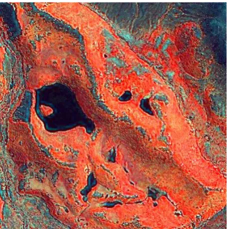
Figure 3-4: Screen captures from an example usage scenario. (a) false colour display of Landsat TM image of Hobart, TAS. (b) selection of a predefined colour table, (c) unsatisfactory volume rendered output (alpha-enhanced), (d) original region data shown as a point cloud (ungeneralised feature space).

It is predicted that standardising the volume prior to direct volume rendering would alleviate the scaling issue but this has not been implemented in this prototype. The issue of visualising the relationships between clusters still remains. Other means such as boundary representations can easily achieve this.

(42)

the visualisation of regions as point clouds for the purposes of comparison to other surfaces.

3.5.2 Ellipsoids

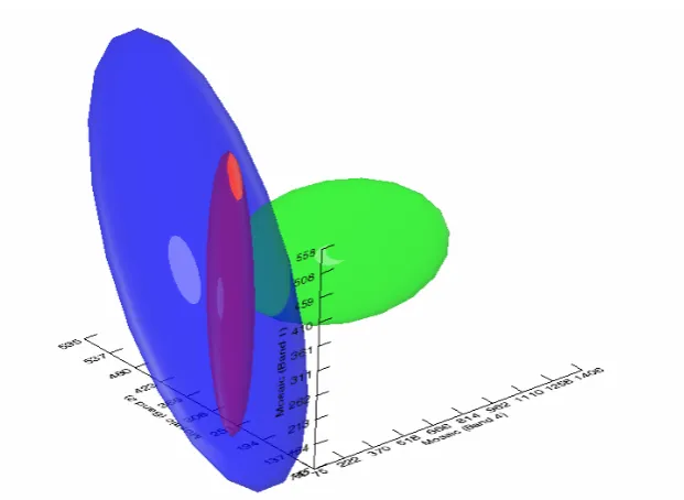
Historically parametric classifiers have been popular in remotely sensed image classification. It is useful to visualise the parameters that will be used for classification. By visualising a statistics based ellipsoid of a data set against the actual shape of the volume as represented by an isosurface or α-shape useful insight into maximum likelihood classification results can be obtained (see Figure 4-13).

A 3D ellipsoid can be constructed based on the statistics of the data set. The mean vector of the data represents the centre of the ellipse. Computing the covariance matrix allows the calculation of eigenvalues and eigenvectors. Eigenvectors can be used represent the direction of the axes of the ellipsoid and eigenvalues to represent the length of those axes. Obtaining these values is known as eigen-decomposition

and can only be carried out on square matrices such as the covariance matrix. Abdi (2007 (in-press)) provides an introduction to eigen-decomposition. The use of these values to reasonably approximate the shape of a cluster relies on the assumption of a normal distribution of points in that cluster.

Figure 3-5: Ellipsoids for regions defined in Figure 3-4a at 60% transparency

3.5.3 α-shapes

(43)

α-shapes can be used to accurately represent the true extent of irregularly shaped or concave clusters. Edelsbrunner & Mücke (2000) state ‘The geometric notion of “shape” has no associated formal meaning.’ They introduced α-shapes as a formal definition and computation of the shape of finite point sets in Euclidean space. For a variable parameter α, shapes produced by this computation range from crude to fine representations of the cluster. This relationship is such that for α = ∞ the α-shape of a point set S is equal to the convex hull of S. As α decreases the shape shrinks and moulds to the concavities of the point set. Tunnels and holes may appear and the connectivity of the shape may be broken as shown in Figure 3-6.

(a) (b)

(c) (d)

Figure 3-6: α-shapes for a sample point set (a), with α values of (b) 784, (c) 100, (d) 50

Formally, if S is a finite point set in Rd (where d is the number of dimensions) and α a real number such that 0 ≤ α ≤ ∞ then the α-shape of S is a polytope (in 2D a polygon or in 3D a polyhedron) that is neither necessarily convex nor connected. Fischer (1994) provides an excellent metaphor for describing α-shapes:

(44)

out all parts of the ice-cream block we can reach without bumping into chocolate pieces, thereby even carving out holes in the inside (eg. parts not reachable by simply moving the spoon from the outside). We will eventually end up with a (not necessarily convex) object bounded by caps, arcs and points. If we now straighten all “round” faces to triangles and line segments, we have an intuitive description of what is called the α-shape of S.

In 3D feature space Rd = R3 as the shape is limited to three dimensions. A graphical illustration of Fischer’s metaphor for a point set in R2 is shown in Figure 3-7. In this case the ice cream spoon is replaced by a simple circle.

Edelsbrunner & Mücke’s (Bloomenthal & Wyvill 1997) algorithm for generating α -shapes takes as input a list of points in Euclidean space; that is, a vertex list and the parameter α. It returns a polygon table defining the faces of the calculated shape.

Figure 3-7: Example formation of a 2D α-shape. The parameter α determines the radius of the disc connecting any two points on the edge of the final shape (Fischer 2000).

(45)

denoted Z3 rather than R3 as the points will be strictly integers. These points make up a cluster which defines the “shape” of the set. In this way α-shapes in the prototype are still tied to the volume representation. This is important as α-shapes are computationally expensive to construct (Lucieer 2004, p. 126). The trade off between detail and processing time based on volume size must still be considered.

α-shapes are implemented in the prototype using hull (Clarkson 2004), an external program written in C. Hull takes as input a list of points in 3D space, that is, a vertex array, and value for α. It produces a list of faces which defines the polygon connectivity for the shape. Each face consists of the three indices of the vertex array in right-handed6 order.

3.5.4 Isosurfaces

A different approach to volume rendering is the extraction of polygonal meshes from the volume data. This gives a surface representation of the volume. Isosurfaces (Bloomenthal & Wyvill 1997) are a popular means of doing this. The surface generated varies depending on a user specified isovalue. Like α-shapes, isosurfaces can be used to represent the extent of clusters in feature space. They also provide a visual measure of the density of the clusters. Unlike α-shapes, isosurfaces require the initial data to be in volume form. The prototype fulfils this requirement by generalising feature space into volume form.

An isosurface can be thought of as a three dimensional isogram (a line connecting points in space having the same numerical value of some variable). A useful analogy is that of isobars on a weather map. Barometric pressure is sampled at various points across the Earth. A grid of dots could be drawn where each dot represents some area on the ground (eg. x km2), Some of the dots would have barometric pressures associated with them (where a measurement has been made). Lines are then drawn through points of equal pressure forming an isobar. Obviously there is not a measurement of pressure for every dot, values are interpolated according to the values of neighbouring recordings. Expanding this to three dimensions (a 3D grid of dots, each representing an area of x km3) it is possible to imagine a value being

6_{In a right-handed system the Z (depth) axis increases toward the viewer. Vertices are ordered}

(46)

available for every point in that 3D space; essentially a volume of barometric pressure readings.

Isosurfaces can be calculated using the Marching Cubes algorithm (Drebin, Carpenter & Hanrahan 1988). The algorithm builds a polygonal mesh according to the specified isovalue. The mesh will represent a surface around or through the volume where voxels have values equal to the isovalue. The effect of the isovalue on the extent of an isosurfaces is demonstrated in Figure 3-8. This can be exploited to visualise where the more dense portions of a cluster lie.

Figure 3-8: Three isosurfaces for a cluster of points in feature space. The Blue surface has an isovalue of 0.1, the green, 0.5 and the red 1.0.

(47)

In order to build an isosurface each point in (ungeneralised) feature space must have a sensible numeric value. This value can be derived in the following manner, as used by (Lucieer 2004): Each pixel when plotted in feature space can be considered a source of gravitational potential energy, analogous to a planet in the universe. In the general case, potential energy (or simply potential) Ug is calculated:

r G U_g ₌₋ m1m2

Equation 3-1: Potential energy in a gravity field

where G is the gravitational constant7_,_m1_and_m2_{are masses and}_r_{is the distance}

between them. This can be simplified for an artificial environment such as a feature space plot:

c g

r U ₌m1

Equation 3-2: Potential energy in feature space

where G = 1.0, m2 = 1.0 and Ug is the potential for a given point in feature space. m1

is the mass of a source determined by the distance to the closest neighbouring source.

c may be used to adjust the power of the potential energy. The potential then for any point in feature space is the sum over all sources of potential for that point. Potential will be high for points near sources and low for points distant from sources. This approach works for feature space plots based on point clouds or other individual pixel representations. This study uses volumes to represent feature space. A small adjustment is needed to generate sensible isosurfaces on these volumes.

The variable m1 can be thought of slightly differently for constructing isosurfaces

based on volumes (eg: a 3D frequency histograms). In this case each non-zero valued voxel in 3D space already represents a cluster of one or more pixels, that is, it has a value that can be treated as the voxel’s mass. Voxels with higher frequencies will cause higher potentials in surrounding voxels of feature space.

(48)

Isosurfaces are commonly generated using the marching cubes algorithm (Lorensen & Cline 1987). This divide-and-conquer algorithm divides space into cubes, similar to the voxels in a volume. Each cube references eight points in feature space, the points at each corner of the cube (Figure 3-9). For each cube, the intersection between the cube and the isosurface is calculated. Intuitively, if one or more of the points has a value less than the isovalue and one or more other points have values equal to or greater than the isovalue then the given cube must contribute some component to the final isosurface. Given this there are an enumerable number of possible intersections within the cube:

Since there are eight vertices in each cube and two slates, inside and outside, there are only 28 = 256 ways a surface can intersect the cube. By enumerating these 256 cases, we create a table to look up surface-edge intersections, given the labeling of a cubes vertices. The table contains the edges intersected for each case. (Lorensen & Cline 1987)

(49)

Figure 3-9: Marching cube (Lorensen & Cline 1987)

Figure 3-10: Symmetrically distinct triangulations (Lorensen & Cline 1987)

Having determined the cube configuration, polygons are generated and the process repeats for the next cube. After all cubes have been processed the generated polygons are connected into a single mesh by standard triangulation.

In the prototype system, feature space is represented by a volume. Each voxel in the volume can be thought of as a point in the previous description of the algorithm. Isosurfaces are implemented in the prototype using IDL’s built in isosurface construction routine. This routine uses a slight variation on the marching cubes algorithm; until recently marching cubes was covered by a U.S. patent (Cline & Lorensen 1985). The user may visualise as many regions as isosurfaces as they desire.

3.6 Highlighting Conflicting Training Data

3.6.1 Linking Data Spaces

(50)

The figures shown in this section are derived from regions within the Hobart Landsat TM image as shown in Figure 3-11. These regions are selected by visual inspection and bear no association with any ground truth data for the region. The purpose is not to verify the correctness of any classification based on these regions, but is to serve as sample data for visualisation in feature space. Indeed figures in this section highlight the vast overlap between the regions.

3.6.2 Limitations

(51)

(a)

(b)

Figure 3-11: ENVI display showing: (a) Landsat TM image of Hobart, TAS annotated with various regions. (b) Colours of regions and their assigned labels.

(52)

Figure 3-13: Feature space intersection between yellow and black regions shown as red (all as isosurfaces with isovalue 0.1) with a volume size of 32.

3.6.3 Determining Pixel Values

Recall that volumes are constructed from an array of pixels of size 3 x n where n is the number of pixels in a given ROI. For a given pixel x in the region, its three component values will be [0,x], [1,x] and [2,x]. This pixel will be referred to as pixel number x in the region. To construct the volume each pixel component must be scaled to lie between zero and the volume size and be converted to an integer value. This produces an array of 3D indices into the volume, one triple for each pixel in the pixel array, which is stored for later use if the user requests the intersection to be mapped to the image display. If a voxel in an intersection volume (the result of intersecting two or more volumes) has a value greater than zero then all pixels falling in that voxel are deemed to have caused that intersection. Pixel values causing intersection (offenders) can then be obtained by the following steps:

1) Use the voxel indices to search the scaled pixel value arrays (one array per volume intersected).

(53)

3) Retrieve the pixels values by indexing the original array using the pixel numbers

Having obtained the list of offenders the prototype then, based on the user’s selection, either:

• Searches the entire image for pixels with values matching any of those in the list, or;

• Searches the regions involved in the intersection for such pixels.

Obviously searching only those regions of concern is vastly more efficient than searching every pixel in the image. The user may wish to use the entire image option to find all occurrences of such offenders. This image searching process is essentially that of Table Look Up Classification (Richards 1986, p. 186).

3.6.4 Displaying Offenders

Section 3.6.3 describes the process of finding the location of offenders. This yields a list of 2D coordinates (x,y) into the image. Pixels at these locations need to be highlighted as they represent uncertain areas in the user’s region selection. The prototype does this by creating a new ROI containing the offending points. The prototype uses ENVI’s built-in routines for creating ROIs from lists of points. This feature is implemented using these functions. The new ROI is assigned an arbitrary colour and unique descriptive label.

(54)

(a) (b)

(c)

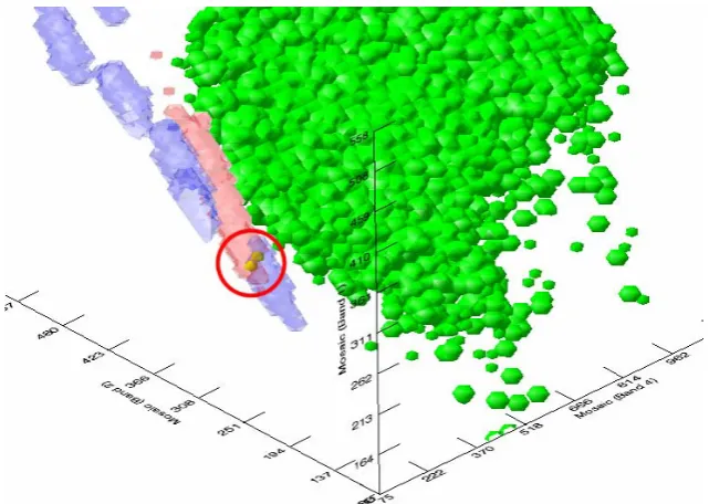
Figure 3-14: (a) Highlighted conflict between regions. Pixels with values that cause intersection in feature space between the City (black) and Suburb (Yellow) classes are highlighted as black points. Spatial intersection is shown as dark red in the City region and green in the Suburb Regions. (b) Zoomed view of boxed area of the image showing spectral intersection between regions. (c) ROI details.

3.7 Configuring the Visualisation

(55)

feature space. ENVI provides the image display and ROI management features. A menu item on the colour composite display launches the visualisation configuration GUI.

This visualisation configuration GUI allows users to select the regions they wish to visualise and the manner in which they visualise them (ellipsoids, isosurfaces, direct volume rendering, etc). It also allows the volume size parameter to be set. Depending on the choice of visualisation type the user may need to specify additional information, eg: isovalues, α values and colour tables for direct volume rendering. The user then clicks a button and the initial visualisation is presented. This visualisation can be rotated, zoomed and panned. The properties (colour, outline style, etc) can be changed from the Visualisation Browser window. This window is part of the iTools framework within which the prototype operates. The user may revise any of their decisions through the configuration GUI at any time.

3.8 Implementation of the Prototype

The prototype system is implemented in IDL using ENVI library functions for image display functionality and classification. The prototype makes use of the iTools

(Intellegent Tools) framework. This means that new visualisations can be easily added; for example, new shapes for cluster representations. In addition to the iTools

framework, RSI also supply a number of existing visualisation programs with the

iTools package. One such program is iVolume, a tool for volume rendering and related operations on volume data. This was used a basis for the prototype, with features such as ellipsoids and α-shapes being incorporated as additional visualisation classes.