Parallelization of the AAE algorithm
By
Akram Hameed (BA-BComp.)
A dissertation submitted to the
School of Computing
In partial fulfilment of the requirements for the degree of
Bachelor of Computing with Honours
UNIVERSITY OF TASMANIA
i
D
ECLARATION
I hereby declare that to the best of my knowledge, this thesis has not been submitted for the award of any diploma or degree at any other tertiary institution. It is also my belief that the thesis contains no previously published material except where due
reference is made.
ii
A
BSTRACT
The exact algorithm formulated by Kececioglu and Starrett (2004) provides a solution to the NP-complete problem of aligning alignments in most biological cases. This work investigates potential speedups that may be gained through the parallelization of the
dynamic programming phase of this particular algorithm. Results indicate it is possible to improve the run time performance of the algorithm over non-trivial alignments that
iii
A
CKNOWLEDGEMENTS
Professor Sale gave me the opportunity to perform this research; so, first thanks go to him for being so optimistic about my ability to do this. Second, huge thanks to Phil for
allowing me to bounce questions off him. Went out of his way to explain things I found perplexing and was always there when I needed to ask a question.
To the academic staff and especially Jacky: your enthusiasm made something
that might have felt like ‘just another year’ into an eye-opening experience. Please keep
up the good work.
And you, gentlemen all of my office – you whom tolerated my vitriolic
conversations with my taciturn console yet spoke not a word of annoyance
yourselves…the office was indeed full of win. Good luck to us all.
My parents were kind enough to do some proofing on this document, as well as lending me a car when I needed to work all night; I owe you guys more than I can repay, I think!
Thanks also go to whoever ended up being in charge of Gundam while the rest of us were busy writing thesis (obscure?).
Finally, I thank my loving wife for having the temperance to hang around while I
finished writing; this may not have taken as long to write as a pHD thesis but I’m
iv
TABLE
OF CONTENTS
:
Declaration ... i
Abstract ... ii
Acknowledgements ... iii
Table of contents: ... iv
Table of Figures ... vii
List of Tables ... viii
1. Introduction & objective ... 1
2. Literature Review ... 2
2.1 Overview: ... 2
2.2 Sequence comparison background issues: ... 2
2.2.1 Background biological concepts: ... 2
2.2.1.1 DNA and Molecular Sequences: ... 2
2.2.2 Parallel and Distributed systems: ... 4
2.2.2.1 Types of Parallel System: ... 4
2.2.2.2 On the Parallelization of Algorithms: ... 5
2.2.3 Objectives of Multiple Sequence Alignment: ... 6
2.2.4 Origins of Sequence alignment: ... 7
2.3 Sequence Alignment Theory: ... 8
2.3.1 Pair-wise Sequence Alignment: ... 8
2.3.1.1 Elements of alignment algorithms: ... 9
2.3.1.2 Substitution Matrices and the Objective Function: ... 9
2.3.1.3 Dynamic programming with Needleman-Wunsch: ... 11
2.3.2 Multiple Sequence Alignment: ... 12
2.3.2.1 Dynamic Programming: ... 12
2.3.2.2 Progressive Alignment: ... 13
2.3.2.3 Iterative Alignment: ... 13
2.3.2.4 Consistency-based Alignment: ... 14
2.4 The Aligning Alignments Exactly Algorithm: ... 15
2.4.1 The problem: ... 15
2.4.2 The exact algorithm (Summary): ... 17
v
2.5 Existing applications of parallel sequence alignment: ... 20
2.6 Summary: ... 22
3. Approaches to Parallelization ... 22
3.1 Considered elements ... 22
3.1.1 Dynamic programming table generation ... 22
3.1.2 Dominance and Bounds pruning ... 23
3.1.2.1 Space reduction under Hirschberg’s principle ... 24
3.1.2.2 Dominance Pruning ... 24
3.1.2.3 Bound Pruning (an overview) ... 26
3.2 Logic & Pragmatism ... 27
3.2.1 Subdividing the Dynamic Programming Matrix ... 27
3.2.1.1 Blocking as an efficiency enhancer ... 27
3.2.1.2 Striping to maximise productivity ... 27
3.2.1.3 Using stripes and blocks to improve timeliness ... 28
3.2.1.4 Speedup of the exact algorithm. ... 31
3.2.1.5 Parallel exact algorithm walkthrough ... 34
4. Method ... 35
4.1 Introduction ... 35
4.2 Metrics ... 36
4.3 Experiment Design ... 37
4.3.1 System architecture ... 37
4.3.2 Assumptions ... 39
4.3.2.1 Networking ... 40
4.3.2.2 Object Serialization ... 41
4.3.3 Calculation of results ... 41
4.3.3.1 Preprocessing of data with ClustalW ... 41
4.3.3.2 Serial AAE ... 42
4.3.3.3 Parallel AAE ... 43
4.3.4 Summary ... 44
5. Results and Observations ... 44
5.1 Performance comparison ... 44
5.1.1 Parallelization overhead ... 44
5.1.2 Small alignments ... 46
vi
5.1.4 Large alignments ... 52
5.1.5 Speed up in general ... 55
5.2 Discussion ... 56
5.2.1 Parallel algorithm performance ... 57
5.2.2 Thresholds and Unpredictability ... 59
5.2.2.1 Unexpected outcomes ... 60
5.2.2.2 Variable block sizes ... 61
5.2.3 Summary ... 61
6. Conclusions ... 62
7. Further work ... 63
8. References: ... 64
vii
T
ABLE OF
F
IGURES
Figure 1:DNA double helix showing base pairing and generic structure. ... 3
Figure 2: Shape propagation in the dynamic programming matrix ... 23
Figure 3: A example of a 5x5 block with numbered cells ... 29
Figure 4: A 4x4 block with logical cached column highlighted ... 30
Figure 5: Input row from a 5x5 block ... 31
Figure 6: 6 stripe by 19 block overlay matrix. Darker shades indicate longer waits for jobs ... 33
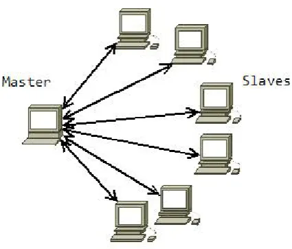
Figure 7: Communication relationship between master and slave cluster ... 38
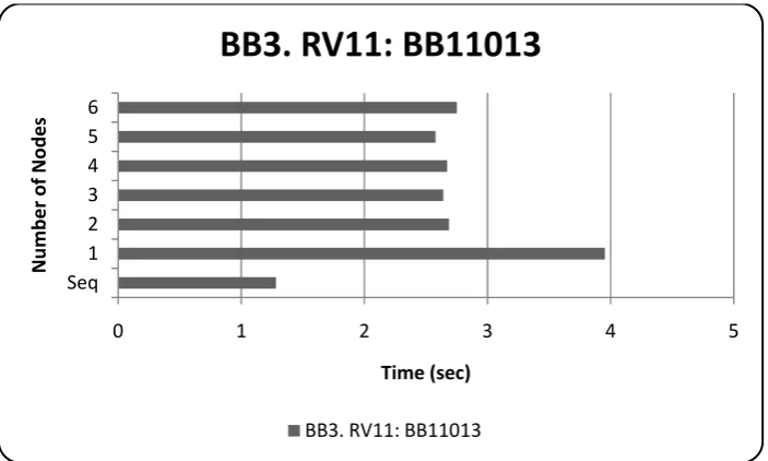
Figure 8: 13th instance of RV11, performance over pUnit scaleup ... 47
Figure 9: 28th instance of RV11 performance over pUnit scaleup ... 48
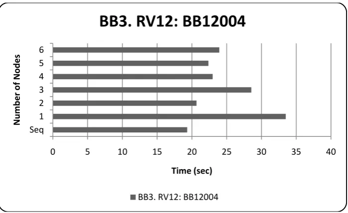
Figure 10: 4th instance of RV12, performance over pUnit scaleup ... 48
Figure 11: 15th instance of RV11, performance over pUnit scaleup ... 50
Figure 12: 43rd instance of RV12, performance over pUnit scaleup ... 51
Figure 13:18th instance of RV12, performance over pUnit scaleup ... 51
Figure 14: 38th instance of RV12, performance over pUnit scale up ... 52
Figure 15: 7th instance of RV12, performance over pUnit scale up ... 53
viii
L
IST OF
T
ABLES
Table 1: Speedup factor as a function of mean processing time over RV11 ... 45
Table 2: Speedup factor as a function of mean processing time over RV12 ... 45
Table 3: Mean run time and speed up over RV1 dataset (‘Small’ range) ... 55
Table 4: Mean run time and speed up over RV1 dataset (‘Medium’ range) ... 55
1
1.
INTRODUCTION & OBJECTIVE
Molecular sequence alignment is a field of bioinformatics that is generally concerned with determining relationships between various organisms (Durbin et al. 1998). This is achieved by analysing the similarities between protein and nucleotide sequences and deriving conclusions about their phylogenetic or even functional properties. This field is
not new; it has existed for over thirty years – however recently it became apparent that
a sub-problem within the field could be rendered soluble given current technology. The
problem was that of ‘aligning alignments’ – the composing of an alignment of many sequences of amino acids or nucleotides from two pre-existing alignments(Kececioglu, J
& Zhang 1998). Despite being proven to be NP-complete (Wang & Jiang 1994), Kececioglu and Starrett formulated an algorithm that solves aligning alignments in polynomial time (2004). Over non-trivial problems, however, the solution may have room for improvement, which leads to the objective of this work:
Investigate the potential for the parallelization of the Aligning Alignments Exactly algorithm and determine the extent to which any parallelization is worthwhile. Given this objective, the following thesis documents research performed upon the exact algorithm with the intention of improving its timeliness through parallelization. Initially, consideration is given to previous work in the field. Following this, an investigation on the pragmatism of parallelization is presented. As a result of the work
undertaken for that section, it was determined that the algorithm could most practicably be parallelized by exploiting the generation of a dynamic programming matrix that forms the core time-consuming activity of the algorithm1
. The approach adopted for examining the extent to which a speedup could be achieved involved the
application of the exact algorithm’s logic in such a manner as to parallelize its core
functions so they may be executed as a distributed application. Tests2
were performed over a number of machines in a micro-cluster in order to determine the extent to which
the hypothesis could be satisfied. The results section3
details the outcome of this research, with a discussion on elements of the findings and a conclusion4
on their validity. Finally, areas that would benefit from further work are mentioned5
.
1 See section 3.1.1
2
2.
L
ITERATURE
R
EVIEW
The first of several chapters investigating the objective stated in the introduction, this literature review does not presume knowledge of the field of sequence alignment, nor that of parallelization. It does, however, make assumptions about the minimum level of
understanding that the reader will have; namely in their comprehension of algorithmic complexity issues.
2.1
OVERVIEW:
The intention of this chapter is to provide grounding in the literature surrounding
multiple sequence alignment. In particular, it examines the Aligning Alignments
Exactly algorithm (hereafter referred to as ‘AAE’) conceived of by Kececioglu and
Starrett for the exact alignment of multiple alignment pairs. Parallelization issues are also discussed in order to support the investigation of the proposed hypothesis that it may be probable to extract a performance enhancement through the parallelization of the AAE algorithm.
2.2
SEQUENCE COMPARISON BACKGROUND ISSUES:
This section considers some of the background concepts of sequence comparison and their origins. A brief overview of the history of sequence alignment is presented with the intention of providing a context for current techniques. Additionally, an introduction to DNA and protein sequences establishes the problem domain for the
research issue.
2.2.1
BACKGROUND BIOLOGICAL CONCEPTS:
2.2.1.1 DNA and Molecular Sequences:
Deoxyribonucleic acid (DNA) molecules play a vital role in the functioning of organic life-forms. Contained within the cells of all known organisms, DNA encodes the information necessary for the production of proteins that enable cells to function and replicate and regulates the
articulation of said proteins to produce an organism’s genetic
3 (Alberts et al. 2002). The alignment of molecular sequences is
traditionally performed upon nucleotide6 or protein sequences.
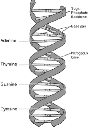
Fig 1. shows a simplified representation of the model of DNA that Watson and Crick proposed (1953). Visible
are the nitrogenous bases that comprise the articulated
‘alphabet’ of DNA. It is these bases, Adenine (A), Thymine (T), Guanine (G), and Cytosine (C) which pair to form the structure of DNA.
As mentioned, they form an alphabet of sorts. If the English alphabet contains 26 characters, the DNA base alphabet contains just the four
specified. Both nucleotide and protein sequences are represented by long text strings. Evolutionary events such as the insertion, substitution or deletion of genetic material are modelled by placing gaps in the place of characters that prevent a
‘best’ alignment (Mount 2001). Before continuing, it would be instructive to mention that protein sequences are sequences of amino
acids which themselves are coded from DNA bases; one example might
be the amino acid ‘Arginine’ which can be coded from cytosine, guanine
and adenine or more simply CGA. Such a triplet of nucleotides in a particular coding sequence is called a codon (King & Stansfield 1997). There exist 20 amino acids that are biosynthesized in protein sequences, each of which have an English character assigned to them for the purposes of protein sequence analysis and alignment (Campbell, Reece &
Meyers 2006).
6 Nucleotide, n. One of the monomeric units from which DNA or RNA polymers are constructed,
consisting of a purine or pyramidine base, a pentose, and a phosphoric acid group (King & Stansfield 1997).
[image:12.595.202.374.152.400.2]4 Therefore, the comparison and subsequent alignment of biological
sequences with respect to this research refers to the comparison of nucleotide or protein sequences. Important issues that should be articulated before proceeding are:
• Given a series of sequences to align, it may become
necessary to substitute characters to obtain the ‘best’
alignment. The caveat of this particular operation is covered in section 2.3.1.1.
• Nucleotide sequences are often measured in terms of base-pairs (bp), the number of which may dictate the mechanism used for sequence alignment.
• The optimality of an alignment of sequences is dependent on several factors that are discussed on section 2.3.
2.2.2
PARALLEL AND DISTRIBUTED SYSTEMS:
The parallelization of a task refers to the subdivision of a given problem into n-units which may be processed in parallel to produce a satisfactory solution (Wilkinson & Allen 1998). The notion of dividing work up to be computed in
parallel is not a new one. A classic example is the work of Holland, who conceived of a system which might allow for the simultaneous execution of many sub-programs, therefore foreshadowing contemporary operating systems with his vision (1959). In the context of sequence alignment, the hypothesis stipulates
that it may be possible to obtain performance gains by parallelizing the AAE algorithm. Prospective gains, however, are dependent on the resolution of several issues which the following sections introduce.
2.2.2.1 Types of Parallel System:
Algorithmic parallelization generally falls between two poles of data parallelization and task parallelization. The former, data parallelization refers to a given data source being processed using the same technique on each node in the parallel architecture (whether those nodes are whole systems or just processors) (Wilkinson & Allen 1998, p. 5). An example
of data parallelization is the Seti@home project: each computer running the Seti screensaver performs the same algorithm on its discrete portion
5 al. 2002). Task parallelization refers to the alternative scenario where
several nodes may execute different algorithms on the same data source, or alternatively on several data sources. Such parallelization is present in the functioning of multiple-core PCs presently, provided that the operating system supports the execution of two tasks in parallel. The historical alternative to task parallelization has been complicated
time-sharing arrangements, whereby a system gives the impression it is
running several programs concurrently, when in truth – the processor
may only execute a single instruction at a time (Zomaya 1996, p. 6).
2.2.2.2 On the Parallelization of Algorithms:
The primary concern of the hypothesis is the possibility of formulating a
parallel version of the AAE algorithm that displays a worthwhile improvement in processing time. Therefore, consider the factors involved in parallelizing algorithm. The speedup factor of an algorithm is defined as:
Where is defined as the run time of the best sequential algorithm and
is the run time of the parallelized algorithm. Zomaya (1996, p. 14)
quite astutely states that the best possible improvement would be that of
given processing units. This presupposes that the problem may be
decomposed into tasks, therefore suggesting that a factor of is the
optimal speedup. Amdahl (1967) theorized that this maximum would be limited by the amount of inherent parallelism in the algorithm itself.
An additional factor that must be considered is that an improvement in computational throughput is often outweighed by the cost of communication between processing units. This is formalized in the ratio:
Where is the communication penalty on processor , is the time
processor i takes to process the algorithm, and represents the time
6 Wilkenson and Allen (1998, p. 26) point out that will have a value
dependant on the granularity of the parallelism inherent in the algorithm. In this circumstance, granularity may be defined loosely as the amount of work processed before another communication interval is required. Therefore, coarse granularity refers to relatively large processing time periods, while fine granularity is the opposite; taking only a modest period to process (Wilkinson & Allen 1998). A final issue that is worth considering is resource utilization; especially given that the most effective versions of the AAE algorithm require quadratic space (see section 3.1.2). Depending on how a resource is defined (whether a resource be a processor or memory); the following metric may be of some utility:
Where is the resource utilization factor, is the number of
operations performed by an -processor machine and represents
the maximum number of operations that might be performed given
processors and time units (Zomaya 1996, p. 15). Stated simply,
represents a percentage of resources utilized during a given parallel process. Clearly, when designing a parallel algorithm, time must be spent considering these issues in order to maximize expectant outcomes.
2.2.3
OBJECTIVES OF MULTIPLE SEQUENCE ALIGNMENT:
Before considering any algorithmic details, it is instructive to examine the uses of multiple sequence alignment (hereafter referred to as MSA) in the laboratory.
Mount (2001, p. 142) suggests that sequence alignment may be used to infer phylogenetic7
relationships between the sequences being aligned. He also proposes that structural or functional attributes can be determined through rigorous analysis of conserved or similar regions of sequences. Further support is provided by Schmollinger et al (2004, p. 1) who state that sequence alignment
has been used recently to determine functional elements of biological sequences. Wholesale explanation of this subject area is beyond the scope of this paper, thus curious readers would be advised to consider the subject matter in the attached
7 Phylogeny: n ‘the pattern of historical relationships between species or other groups resulting from
7 reference list. The following section examines the origins of sequence alignment
and its most influential architects.
2.2.4
ORIGINS OF SEQUENCE ALIGNMENT:
The 1970s saw what Baxevanis and Ouellette describe as an ‘explosion’ in the
number of DNA sequences that became available for research (2001, p. 145). Comparison and alignment of available sequences was theorized as a productive method of analysis. One such algorithm, the Needleman-Wunsch algorithm was proposed by Saul Needleman and Christian Wunsch in a seminal 1970 paper. Needleman-Wunsch envisages a dynamic programming approach to sequence alignment, effectively producing what is known as a global sequence alignment. In such an alignment, the entirety of a biological sequence (whether protein sequences as in the original paper, or nucleotide sequences such as DNA more recently) is aligned with the intention that further analysis of the combinate sequence will reveal useful genetic relationships. Given that the dynamic
programming approach is a key element in the AAE algorithm, section 2.3.1.3 provides a brief overview of the intrinsic nature of the Needleman-Wunsch algorithm.
In 1981, building on Needleman and Wunsch’s work and incorporating
some tenets of Hirschberg’s (Hirschberg 1975) maximal common subsequence
theory, Temple Smith and Michael Waterman proposed a method for finding local sequence alignments. Such a method is often employed when the evolutionary distance between sequences is large and the probability of highly
conserved8 regions in the sequences is remote. Buoyed by the success of pair-wise alignment researchers conceived of the benefits of comparing several protein or nucleotide sequences, and hence the theory of aligning multiple sequences emerged in the late 1980s. Since then, many researchers (Collins & Coulson 1984; Myers & Miller 1988; Needleman & Wunsch 1970; Smith & Waterman
1981) have attempted to render the problem into an optimally solvable state, though it is arguable that at present, optimal alignments may be achieved only at the expense of great amounts of time and resources (Kececioglu, J & Starrett 2004; Schmollinger et al. 2004). As a computationally feasible alternative,
8 In this circumstance, the level of conservation of a region belonging to a sequence is the probability that
8 optimal but efficient methods have grown increasingly popular, as will become
evident in the subsequent section on MSA strategies.
2.3
SEQUENCE ALIGNMENT THEORY:
The alignment of nucleotide and protein sequences has been claimed to allow researchers to identify homologous regions in the genetic makeup of many species (Mount 2001).
The term ‘homology’ refers to conclusions that the genetic material examined shares a
common evolutionary history, something that is often considered to be a desirable
attribute of sequence alignments (Baxevanis & Ouellette 2001). The field may be divided into approximately two sub-fields: first is pair-wise sequence alignment where two sequences are aligned using various mechanisms; second is multiple sequence alignment, where 3 or more sequences are aligned. Alignment algorithms may be divided into several types: those that attempt to construct a mathematically optimal
alignment, and those that attempt to construct a best-possible alignment using alignment heuristics. Baxevanis and Ouellette inter alios caution that the optimal mathematical alignment is not necessarily the best possible biological alignment in terms of simulating expected evolutionary events (2001, p. 151; Mount 2001, pp. 64-65).
2.3.1
PAIR-WISE SEQUENCE ALIGNMENT:
Computational sequence alignment began with pair-wise sequence alignment.
The Needleman-Wunsch algorithm (Needleman & Wunsch 1970) allows for optimal global alignments to be achieved and in its original form, required
approximately steps in the worst case, and space requirement of
where and represent two molecular sequences, the latter being the
9 2.3.1.1 Elements of alignment algorithms:
The alignment of molecular sequences tends to require different elements
depending on whether one wishes to align protein sequences or nucleotide sequences. Given an alphabet of characters from which sequences may be constructed, alignment algorithms generally define a character to fill
the ‘gaps’ in the sequence which define homologous regions (Durbin et al.
1998, p. 13). Another element that is common is a substitution matrix; the substitution of one amino acid (or indeed, the substitution of one DNA base) for another may improve or degrade the optimality of an
alignment, but may alter the inherent meaning or function of the genetic code (Gusfield 1997). As such, the substitution matrix is a construct
that provides a ‘cost’ for the substitution of characters. Substitution
matrices are usually crafted by experts in molecular biology, rather than
computer scientists (Mount 2001). Substitution ‘cost’ is often used along
with a cost defined for inserting a ‘gap’ to determine the optimality of an
alignment. Gaps, however, may run for more than a single character, so algorithms like the Needleman-Wunsch algorithm (1970) also define a gap-extension cost which is summed with the gap-initiation cost already mentioned, and finally used to compute alignment optimality. Further
explanation of these terms and elucidation of the mechanisms used to define them may be found in (Baxevanis & Ouellette 2001; Durbin et al. 1998; Gusfield 1997; Mount 2001).
2.3.1.2 Substitution Matrices and the Objective Function:
As mentioned, substitution matrices are used to calculate the ‘cost’ of
substituting one character for another in sequence alignment. This
theory can be traced back to the work of Dayhoff, Eck and Park (1972), who conceived that to model evolutionary events, such as the insertion or deletion of genetic material, it would be of some utility to assign a probability to the likelihood that a pair of sequences were related or not.
The point-accepted-mutation (PAM) model of evolution that Dayhoff and his counterparts published is a widely used set of substitution matrices for amino-acid (therefore, protein sequence) comparison.
Baxevanis and Ouellette put the definition of PAM quite simply: ‘one
10 have been changed.’ (2001). The Dayhoff process model, itself a Markov
process, dictates that given an amino acid the probability of mutation
to any other amino acid in an alphabet Ζ is independent of any other mutations which may have occurred at other sites in the protein (Mount 2001, pp. 83-84). This assumption that each amino-acid position is equally mutable is open to conjecture and has been challenged (George, Barker & Hunt 1990). Complementary to the concept of substitution
matrices, is the objective function that calculates the quality of the obtained alignment. For multiple sequence alignment, a common (and in our case, used in the AAE algorithm) choice has been the sum-of-pairs objective function. This is defined by Pevzner as the following (2000, pp. 125-126):
‘For a multiple alignment , the induced score of pairwise alignment for sequences and is
, ,
Where is the distance between elements of any alphabet…’ Ζ given
Ζ (assuming – represents a spacer character not in the original
alphabet Ζ.). Given this expression of a pair wise alignment, the sum-of-pairs score (SP-score) may be calculated using the following expression:
, .
Or more simply, according to Gusfield (1997, pp. 343-348), SP-score is equivalent to the sum of the scores of pair wise global alignments induced
by some multiple alignment . The complexity of calculating the
SP-score for a worthwhile problem exactly is defined by Wang and Jiang (1994)to be NP-complete. An explanation of how this is expressed is not relevant to the research issue; therefore the enterprising reader may find a full dissertation in the referenced paper. The combination of
11 given substitution matrix depends on the hypothetical relatedness of the
sequences to be compared (Mount 2001, p. 83).
2.3.1.3 Dynamic programming with Needleman-Wunsch:
In the interests of providing a clearer explanation of the AAE algorithm, an overview of the original Needleman-Wunsch algorithm follows:
Initially, given two sequences and of lengths and respectively,
construct a matrix that may be denoted as . For clarity’s sake,
assert that consists of columns and rows. Let , be a function to represent the edit distance between the first characters of
and the first . The definition of edit-distance with relation to sequence
alignment may be seen as the number of operations required in order to
‘merge’ the two sequences and . Gusfield defines the dynamic programming approach as having three components – ‘the recurrence relation, the tabular computation, and the traceback’ (1997, p. 217). Furthermore, define the scores for the edit-distance metric to be 1 for
mismatches or gaps and 0 for matches. A recurrence relation for , may be established as the following:
min 1, 1, , 1 1, 1, 1 , ,
Where , is defined as having a value of 1 if , or a value
of zero if . Using this recurrence relation, the second
component of the dynamic programming approach is satisfied: tabular
computation. The simplest method of composing the dynamic programming table is to use the recurrence relation and establish
0 & 0 0 (assuming the comparison of elements begins at
12
, and searching back through the matrix, ascertaining at each step precisely which value the current value was calculated from. This is
akin to storing a series of pointers from cell to cell – essentially, given the
recurrence, when , is computed, set a pointer from that cell to cell
, 1 if , , 1 1; set a pointer to 1, if
, 1, 1; and set a pointer to 1, 1 if ,
1, 1 , (Gusfield 1997, p. 221). In essence, conduct a traceback storing pointers indicating the direction that the minimal values were found. As mentioned, the dynamic programming approach is
utilised in the AAE algorithm – namely the concept of using a table to
store sequence identities9
and conducting a traceback to obtain an optimal alignment.
2.3.2
MULTIPLE SEQUENCE ALIGNMENT:
As mentioned, the alignment of multiple sequences is a significantly more difficult problem than that of pair-wise alignment. As such, there are many
mechanisms employed to achieve an alignment, each differing in their implementation. The key methods are listed below, though several key elements of MSA are discussed before continuing.
2.3.2.1 Dynamic Programming:
Pair-wise alignment can be achieved through dynamic programming
practices with an approximate complexity of between and
(Needleman & Wunsch 1970). Multiple sequence alignment is considered to be a significantly more difficult process; if we take our example of using dynamic programming and conceive of a k-dimensional version of the original Needleman-Wunsch algorithm, it has been shown
to have a space cost of and a time cost of 2 where there are k strings (sequences) of length l (Durbin et al. 1998, p. 142; Gusfield 1997, p. 344). While cunning attempts have been made by researchers to
improve the performance of dynamic programming methods on multiple sequences (Carrillo & Lipman 2006; Gupta, Kececioglu & Schaeffer
9 Identities in the case of dynamic programming refers to obtained scores, in the case of the AAE
13 1995), the number of sequences it is possible to align using this method
in a reasonable timeframe is assumed to cut off at 7 (Durbin et al. 1998, p. 142; Gupta, Kececioglu & Schaeffer 1995).
2.3.2.2 Progressive Alignment:
The runtime cost of dynamic programming techniques encouraged
researchers to approach the process of sequence alignment from different perspectives. Progressive alignment is a hybridized approach whereby multiple sequences are aligned incrementally, generally by continuous pair-wise alignments (Mount 2001, p. 152). Durbin et al.(1998, p. 144)
suggest that there are three ways such progressive methods differ from one another; first of all, the initial logic they employ to order the sequences being compared. Second, whether the phylogenetic10
tree that is created during processing involves a single alignment or several sub-related alignments. Finally, they may differ in the procedure and heuristics used to score sequences and alignments against one another.
Despite the ability of such progressive systems to compute a significant number of sequences into a multiple alignment, Mount (2001, p. 155) cautions that the result is not guaranteed to be an optimal alignment. One example of a popular progressive alignment system is:
ClustalW: A system whereby sequences are progressively aligned in a pair-wise manner, with weighting selectively applied to sequences and substitution costs in order to create the most accurate alignment. Further explanation can be found in (Thompson, Julie D., Higgins & Gibson 1994).
2.3.2.3 Iterative Alignment:
The iterative approach to MSA attempts to address the problems inherent in the progressive alignment process; namely that the quality of the final MSA rests heavily on the quality of the initial alignment and
the order of subsequent pair-wise alignments (Gotoh, O. 1996). As suggested by its name, such an approach repeatedly re-aligns regions and subgroups of sequences so as to provide a global alignment that is more
14 optimal than would be produced had such optimization not been
performed. One well-known iterative system is:
DIALIGN: A program conceived of by Morgenstern inter alios (1998) that attempts to create optimal global alignments via progressive alignment and then iterative weighting of local regions (or motifs11).
According to the authors, DIALIGN contrasts itself from more
traditional methods by ensuring that the local similarities between sequences are used to construct an MSA that displays an alignment that
‘maximizes the sum of individual similarity scores’ (Morgenstern et al. 1998, p. 293).
2.3.2.4 Consistency-based Alignment:
An element of most alignment strategies is the substitution matrix. As mentioned, often the measure of goodness for a particular alignment may be biased depending on the particular substitution matrix employed. Consistency-based alignment strategies may employ the methods used by the previously mentioned approaches (exact, progressive, and iterative)
to construct pair-wise alignments. At this point, the similarity to these employed mechanisms diverges; the measure of goodness employed by consistency schemes defines the optimal MSA to be one that is most representative of all possible pair-wise alignments in a given set of sequences (Notredame 2002). Unfortunately, according to Kececioglu,
computing such an optimal alignment is an NP complete problem (1983). One well known MSA application that employs the principles of
consistency-based alignment is T-Coffee. The basis for a residue pair’s
score is given by what Notredame et al refer to as a ‘position-specific
scoring scheme’. Pair score is dictated by the compatibility of the given
pair with the sequences that comprise the library of weighted pair-wise
alignments generated in the initial stages of T-Coffee’s alignment process
(Notredame, Higgins & Heringa 2000).
ap11 Motif here refers to a ‘sequence motif’, that is, a recognizable pattern in a nucleotide or amino-acid
15
2.4
THE ALIGNING ALIGNMENTS EXACTLY ALGORITHM:
The AAE algorithm as previously mentioned is an approach to MSA. It concerns in particular, the alignment of two multiple sequence alignments (Kececioglu, J & Starrett
2004). The algorithm is claimed by Kececioglu and Starrett to be capable of producing optimal alignments on benchmark instances in two widely used datasets. This claim might appear curious, given their complementary statement that aligning alignments is NP-complete, however they go on to emphasize that while the problem is inherently hard in the worst case, it is possible to produce a polynomial-time solution in practice. What is perhaps most interesting about AAE is that it claims to be able to produce optimal alignments, which are by their very definition, desirable to researchers.
A detailed explanation of the exact algorithm in the space available is infeasible, however the problem behind AAE is discussed in some detail in section 2.4.1 and a summary of the solution is provided in section 2.4.2. Initially however, it is instructive to consider some elements of the AAE algorithm itself.
First of all, the product of AAE is an optimal alignment of the two input MSAs, being able to handle instances with approximately 100 sequences consisting of 1000 columns (2004, p. 95). Second, these optimal alignments may be achieved using a
technique Kececioglu and Starrett refer to as ‘dominance pruning’ (2004, p. 94) that
allows for computation in linear space. Furthermore, the application of the proposed
‘bound pruning’ (2004, p. 95) technique, may decrease the time complexity by an order of magnitude while having the side effect of increasing space cost to quadratic. Finally,
the exact algorithm has been rigorously tested on two independent benchmark datasets(2004, pp. 92-94); namely the BAliBASE and that of McClure, Vasi, and Fitch (McClure, Vasi & Fitch 1994). The results presented by Kececioglu and Starrett provide plausible substantiation that the AAE algorithm is effective in practice, despite its worst-case complexity. Let us now examine AAE in order that a methodology may
be derived for investigating the hypothesis.
2.4.1
THE PROBLEM:
Kececioglu and Starrett (2004, p. 86) define the problem of ‘Aligning
Alignments’ as:
16 , substitution cost function , gap initiation cost , and gap extension cost .
The output is an alignment of the columns of versus the columns of that
minimizes the sum-of-pairs objective with linear gap costs.”
This formidable definition contains several key elements:
• Alignments and are defined as being multiple alignments if
and only if any collection of strings which may be composed
into an alignment contains more than two strings.
• Any string in alignments and (therefore, from collection )
may contain only characters from a given alphabet or a spacer
(gap) character, which is denoted as ‘-‘.
• An assumption is made that such gaps may run for one
column. Hence, the cost for any given gap of length is defined
as where is a constant 0 that is defined as the cost of initiating a gap, and 0 is the cost of extending a gap.
• Given that substitutions will undoubtedly occur, it is necessary to
define a substitution cost function δ that assigns each pair of
letters , the cost , , . Therefore, define
alignment cost as the sum of all substitution costs , over
all non-gap columns , plus the sum of the gap costs.
• The sum-of-pairs objective scores a given multiple alignment A in
the following manner. Given two rows , in alignment A, induce a pair-wise alignment of the strings and . A weight
function is defined to assign each pair of strings , the
weight , , .
According to the authors, therefore, the sum-of-pairs cost of alignment A is
defined to be the weighted sum of the costs under cost function of the two
17 weighted by , . Hence, the pair , specifies the sum-of-pairs objective function (Kececioglu, J & Starrett 2004).
2.4.2
THE EXACT ALGORITHM (SUMMARY):
The AAE algorithm essentially follows the dynamic programming method as originally presented by Needleman and Wunsch (1970). This is with respect to its representation, as we view the alignments as a series of columns. Therefore,
in order to align an alignment of rows and columns to an alignment of
rows and , AAE requires the construction of a grid-structured graph of
dimensions 1 by 1. Next, the graph is examined in lexicographic order, which corresponds to traversing the graph in row-major order until the cell
, has been calculated.
To determine the cost of any alignment the exact algorithm produces, it is necessary to establish the number of gaps initiated by a given column. The proposed theory for doing this rests on the concept of a shape. Shapes are ordered partitions of the rows of both alignments, indicating the ordering of each
row’s final character. This is most easily explained with an example; consider
the shape 4 2 , 1,3 – each number in this construct represents a pair of rows in a given alignment such that row 4 finishes first, with its last character
followed by gaps, row 2 finishes second, while rows 1 and 3 finish after both 4 and 2, however in this particular shape, rows 1 and 3 end in the same character
(either a letter or a gap) and as such are called ‘flush’. The algorithm dictates in
this circumstance that row 4 underhangs rows 2, 1 and 3, and row 2 overhangs row 4 respectively. Because there may be multiple alignments generated during the alignment process, each cell in the dynamic programming table maintains a
list of shapes and scores for the optimal alignment that ends in that particular shape.
Given the ability to generate shapes and the multiple alignments and
that were of sizes and respectively, the optimal alignment of and is generated by solving the following subproblem: for any shape and
indices 0 and 0 , the cost of an optimal alignment of the
18 aligning all given prefixes. . Hence, set of all possible alignments given these
prefixes is denoted as , for a particular cell in the dynamic programming table. The cost of an optimal alignment of and is defined to be:
min
s S m, n C m, n, s .
In order to count gaps the following predicates are employed:
For a pair of rows and in an alignment with shape .
qsp if and only if p overhangs q in the alignment, and psq if and only if p underhangs q.
And for the rows p and q and a column c,
qcp if and only if p has a letter and q has a spacer in column c, and pcq if and only if q has a letter and p has a spacer.
Thus when aligning two columns and , the composite column is formed by
placing on . Using this notation, and will columns from or or
alternatively, a column of all spaces (gaps). So, the total number of gaps that
are initiated by appending column , onto any new alignment that ends in shape is:
, , , ! , ! .
Assume in this equation that any predicate that evaluates to true is equal to 1, and the opposite evaluates to 0. A ‘flat’ shape is defined to be a shape in which all rows are flush, where the associated alignment concludes with a column composed of all letters, or is empty altogether:
1, … , .
19
,
, 0 0; , 0 0; 1, , , 1 ,
1, 1 , , .
Where , is the set of all shapes at any given cell in the table, and given a column , is the shape derived from concatenating onto an alignment ending in shape . Therefore, , is the set of shapes derived from
concatenating onto any such that , . Assume in this circumstance also, that any refers to any column in alignment , and refers to any
given column in alignment . Once , is established, the sub-problem of
, , must be solved. The recurrence for , , relies on the assumption
that the optimal alignment of 1: and 1: ending in shape must have the final column such that with the removal of an optimal alignment remains
that ends in shape š where š . Hence assuming 0 and
0 , and , , and , ! 0,0 :
Where | | denotes the number of letters in column . Therefore, for ,
20
0,0, 0.
2.4.3
BENCHMARK TEST SUITES:
For the purposes of this research, test data will be instrumental in determining whether the objective has been achieved and has satisfied the demands of the
hypothesis. Given the problem domain, it would be most instructive to utilize the test data that was used to determine the performance of the exact algorithm in the first place. As such, any experimental system will be tested on the BAliBASE test suite. BAliBASE is specifically designed to allow for the benchmarking of MSA algorithms (Thompson, J. D., Plewniak & Poch 1999)
and has evolved considerably since its inception (Julie D. Thompson 2005). The referenced papers provide an excellent overview on the constituent elements of BAliBASE and its adoption rate since it was published in 1998. One other documented set of test data that Kececioglu and Starrett tested AAE on is that of McClure, Vasi, and Fitch (MVF) (1994, p. 573). While the MVF dataset was carefully selected to provide a fair analysis of MSA applications, the difficulty of
obtaining the original dataset and its age in comparison to the BAliBASE (given that BAliBASE has been maintained and improved upon since its inception) renders the MVF to be a less attractive candidate for use as test data. The architects of BAliBASE (Thompson, J. D., Plewniak & Poch 1999) clarify the
need for distinct databases of accurate reference alignments for the use of testing MSA programs given that MSA algorithms by their very nature require more than two sequences to produce a compelling alignment. They stipulate that the
performance of an alignment program rests upon ‘the number of sequences, the
degree of similarity between sequences and the number of insertions in the alignment. Other factors may also affect alignment quality, such as the length
of the sequences, the existence of large insertions…’ (1999, p. 87).
2.5
EXISTING APPLICATIONS OF PARALLEL SEQUENCE ALIGNMENT:
Given the hypothesis, it is instructive to examine previous examples of parallelised sequence alignment methods. Perhaps unsurprisingly, most examples of parallel sequence alignment (at least, in the area of MSA) attempt to parallelise either progressive or iterative alignment algorithms (Ebedes & Datta 2004; Li 2003; Schmollinger et al. 2004; Yap, Frieder & Martino 1998). What is perhaps more useful
21 given that it is an integral part of the AAE algorithm. Typical parallelization methods
for the dynamic programming approach are usually concerned with applying the
approach to comparing a single sequence against sequences (Brutlag et al. 1993;
Trelles-Salazar, Zapata & Carazo 1994);this is due to the practical concerns of searching databases for particular sequence similarities. Parallelization of the actual algorithm itself (and not the large-scale application of the algorithm) is a less well-studied field. Martins et al. (2001)discuss a method whereby it is possible to parallelise the composition of the dynamic programming table. They suggest three possible methods of parallelising this particular step in the algorithm. In particular, given that the value of
any cell is dependent on its north, north-west and western neighbour cells:
Parallelise the computation by allocating a processor to each row, using discrete time
intervals to co-ordinate communication.
Perform a similar operation, only on the columns of the table rather than the rows. Or, anti-diagonal by anti-diagonal, allowing the computation to progress in the original top-down method.
The initial two approaches are discarded by Martins et al. due to the fact that elements within a given row or column depend on other elements within that same row or column. Hence, it is not possible to parallelise the composition of individual rows or columns (Martins et al. 2001). The third approach minimises this problem in that any
diagonal is dependent on only the three neighbours as mentioned above. Problems
inherent in this approach are communication costs; all processing units would need to communicate among one another in a somewhat complicated fashion. Also, assuming that each processor calculates only one value in the table, it requires three input values
and creates only one output value; a 3: 1 communication to computation cost. Martins et al. (2001) circumvent this overhead by performing a block division upon the table whereby a certain range of elements are assigned to a given processor to be computed at any single time step. Dependencies still exist with this method, however communication
overhead is reduced: assume each block contains 4 4 rows and columns respectively – said block requires 9 input values (those to the west of the block, those north, and a single element in the north-west), yet computes 16 minima, dropping the communication to computation ratio to 9: 16. Further improvements are also mentioned, namely the horizontal striping of the block table in order to alleviate
22 own hypothesis, given that one of his aims was performance enhancement on general
purpose parallel computing platforms.
2.6
SUMMARY:
This review has presented an introduction to the relevant issues pertaining to the investigation of the stated hypothesis. An attempt was made to relate the field of
sequence alignment theory to the issues inherent in the parallelization of applications. A parallel version of the Needleman-Wunsch algorithm was examined that may provide some insight into the investigation of the current hypothesis. Naturally, given the scope of the review it is impossible to explain exhaustively all relevant issues, though attempts have been made to direct curious readers towards the appropriate resources. At each
stage it was necessary to consider the utility of a particular subject area given the hypothesis. Subsequent chapters discuss the method employed for the parallelization of the AAE algorithm and what results have been gathered.
3.
APPROACHES TO PARALLELIZATION
This chapter deals with the approach taken to parallelize the AAE algorithm. Initially, it describes the issues with the algorithm that prevent it from being embarrassingly parallel and how these may be alleviated to successfully parallelize one particularly time consuming operation. The choice of this particular operation as a suitable candidate for parallelization is discussed in the second section, as is the motivation for using the dominance pruned variant of the algorithm during this research.
3.1
CONSIDERED ELEMENTS
3.1.1
DYNAMIC PROGRAMMING TABLE GENERATION
Kececioglu and Starrett (2004) describe the initial stage of the AAE algorithm as
using a dynamic programming table. This matrix is the same grid-structured graph described in section 2.4.2 and is composed over the columns of any two
alignments and . For each entry , in the table a list of shapes is maintained, the generation of which comprises the initial stage of the algorithm.
Given that in the worst case the number of shapes at an entry is exponential in
and (where and are the number of sequences in the alignments and )
the problem of computing this matrix is not trivial.
23 in section 2.5, Martins et al (2001) had some success with their parallelization of
the computation of a dynamic programming matrix. They observed that any potential speedup factors would be confounded by the dependencies present in the underlying algorithm; dependencies which exist through generalisation of the dynamic programming approach, in the AAE algorithm. This corresponds to the necessity of computing the shape-list of neighbouring cells to the north,
north-west and west of any cell before the computation of may commence.
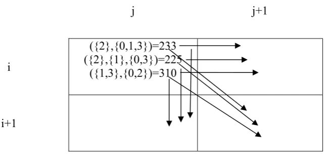
Figure 2 demonstrates this relationship, with each arrow corresponding to a required propagation of a shape. In the context of the exact algorithm, the relative finishing order of each arrow in the figure dictates the order in which
each shape from the cell , is propagated. This order can be important when deciding whether to maintain a shape in a cell’s shape list, especially when
incorporating a pruning technique into the algorithm.
j j+1
i
({2},{0,1,3})=233 ({2},{1},{0,3})=225
({1,3},{0,2})=310
[image:32.595.204.526.360.519.2]i+1
Figure 2: Shape propagation in the dynamic programming matrix
Section 2.4 mentions dominance and bounds pruning techniques as allowing a substantial reduction in the time and space complexity of the AAE algorithm (in particular, the generation of the dynamic programming matrix); therefore, the theory of these techniques is discussed in the following section.
3.1.2
DOMINANCE AND BOUNDS PRUNING
In order to reduce the time and space complexities of the AAE algorithm and render it useful as a tool for molecular sequence alignment, it was necessary for
24 operations were prevented from occurring. Kececioglu and Starrett (2004)
propose three techniques for improving the performance of AAE.
3.1.2.1 Space reduction under Hirschberg’s principle
The maximal common subsequence theory discovered by Hirschberg (1975) dictates that it is possible to compute an optimal alignment of any
two strings and in space linear in the lengths of and respectively.
Myers and Miller (1988) go further, discussing a generalisation of
Hirschberg’s theory to allow the alignment of two strings with linear gap
costs; an essential step in some forms of molecular sequence alignment. Furthermore, it is possible to generalise this divide-and-conquer approach
to the problem of aligning alignments. Kececioglu and Starrett (2004) describe a method whereby the optimal alignment is produced via a row-swapping approach made possible by the dominance pruning heuristic (see next section). While this has the effect of reducing the space consumption of AAE to linear in the number of columns of the input
alignments, it does not improve the runtime significantly; time complexity remains quadratic in the number of shapes generated during the row-swapping procedure. Nevertheless, this is an attractive mechanism that could be employed if it were necessary to use the
algorithm on a workstation with limited memory.
3.1.2.2 Dominance Pruning
Reducing the space of AAE is an imperative to its successful conclusion; dominance pruning allows for significant space saving while having the
side-effect of improving the timeliness of the algorithm markedly. Essentially; establish a dominance relation that operates on pairs of shapes. As mentioned, each cell in the dynamic programming matrix
represents a list of shapes. Given some cell with associated shapelist
the total number of shapes maintained by the vanilla algorithm is
exponential in the number of sequences, hence where represents the
rows from some alignment and represents the number of rows from
some alignment . This is clearly unacceptable on all but the most
25 and pruning of shapes in such a manner that the resulting shape list is
equivalent to its form if it had been pruned post-propagation. This is established by the following logic. At each stage in the algorithm, from
some location , in the dynamic programming matrix, three operations can be completed; an insertion, a deletion, or a substitution – note that
these operations are those of propagating a shape to the east, south or south east of the current cell. Each of these operations yields a subalignment of the current alignment that Kececioglu and Starrett (2004) term an extension. The dominance pruning technique seeks to
establish a relation where for shape in some list , remove if it is
never better than another shape from the same list over all possible extensions from that cell. Thus, for shape and extension let
denote an alignment derived from composing onto the pre-computed
alignment associated with . Let denote the cost of an alignment
ending in shape , and denote the cost of subalignment that
begins with the flat shape (the initial shape in the matrix – wherein all
sequences finish at the same point and associated cost is 0). Further, let
, represent the count of the numbers of pairs of rows and
such that overhangs or underhangs in a gap that is continued
by . It is possible then to establish:
, .
Where represents the gap initiation cost discussed in 2.4.1. To extend
this, shape is no better than shape on any extension if it is possible
to show the following:
, ,
! !
26 Wherein the definition may be simplified because the resulting upper
bound on pairs of rows that satisfy the overhang/underhang conditions is
independent of . Therefore, shape dominates shape if:
! !
This definition is of particular importance given that it means that in the
best case, the shape-list at a given cell can be pruned to length 1. Note the two fold benefits of this operation; while it requires some overhead to
perform the dominance calculation – it will result in less work over time
given that there will be fewer shapes to propagate, which in turn,
dictates that there will be a lower storage overhead. Furthermore, it is possible to combine dominance pruning with the row swapping space reduction technique mentioned earlier. This is the method by which the algorithm may run in space linear in the number of input columns from
any two alignments and .
3.1.2.3 Bound Pruning (an overview)
Bound pruning seeks to improve the time complexity of the exact
algorithm by computing upper and lower bounds , on the cost of the ‘best alignment of and that extends the alignment associated with shape ’ (Kececioglu, J & Starrett 2004). Unlike dominance pruning, bound pruning cannot be used alongside the row swapping technique,
rendering its space complexity to be where is the number of
input columns from alignments and . One of the benefits of bound
pruning, however, is that unlike dominance pruning, in the best case, the algorithm can prune an entire shape-list from the table, thereby decreasing the amount of work that must be performed during
composition. Unfortunately, bound pruning requires the computation of three tables for optimistic scores; one for insertions, one for deletions, and a final table for substitutions (Kececioglu, J & Starrett 2004). This has the net effect of imposing a great deal of overhead in situations where it would be desirable to subdivide a task for parallel processing. These
27 generation of the dynamic programming matrix) having further
dependencies introduced that render a bound-pruned matrix infeasible to compute over several machines.
3.2
LOGIC & PRAGMATISM
This section examines the logic behind the design decisions made for the parallel
implementation of the AAE algorithm. First is an overview of the approach used for subdividing the matrix into distinct entities that may be assigned to individual processing units; second, justification is provided for the appropriateness of the chosen parallelization scheme.
3.2.1
SUBDIVIDING THE DYNAMIC PROGRAMMING MATRIX
As has been previously mentioned, the most expensive aspect of the exact algorithm is that of composing a matrix of shapes. The time and memory complexity may be improved upon using bound and dominance pruning, however, as stated in the hypothesis; for large alignments it may be possible to improve upon the speed of the sequential algorithm by parallelizing the composition of the shape matrix. The approach taken to improve timeliness has
two aspects.
3.2.1.1 Blocking as an efficiency enhancer
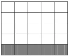
The first aspect is that of dividing the elements of the dynamic programming table into blocks. A block is defined as a subset of cells
from the dynamic programming table, such that ζ where . denotes the set of all cells in some matrix , and ζ denotes a stripe from
the set of stripes Ζ. Stripes are defined and discussed in the following section (3.2.1.2). The following sections also discuss how blocking is used
practically to improve efficiency by aggregating work for processing.
3.2.1.2 Striping to maximise productivity
The second aspect to improving the timeliness of the exact algorithm is that of block striping. In the context of the parallel exact algorithm, a
stripe may be defined as a subset of the rows in some matrix .
28 advantageous to ensure that all processing units (hereafter referred to as
pUnits) are always assigned some kind of work (Martins refers to this
concept as ‘strips’). Stripes are one mechanism whereby it is possible to
maximise processor productivity. Conceptually, assigning a stripe to a pUnit has the effect of making that pUnit responsible for all blocks in the
stripe ζ. The utility of this approach is discussed next.
3.2.1.3 Using stripes and blocks to improve timeliness
Given the definitions of blocks and stripes provided, the question remains how can they be used to practically improve the timeliness of the exact
algorithm? Wilkinson and Allen’s (1998, p. 26) requisite communication versus expected computation ratio (as defined in 2.2.2.2) dictates that in distributed parallel applications, it is beneficial to aim for a ratio that is biased towards a higher expected computation outcome. Essentially, the
algorithm should achieve a processing output that is greater than the required communication for that particular output. In terms of the parallel exact algorithm; both striping and blocking help lower the communication to computation ratio significantly. Recall that each cell in the dynamic programming matrix is dependent on its northern, north-western, and western neighbours for input. Furthermore, these neighbours must be complete in the sense that their shape-lists must be their final length; this is to say, an assumption is made that the shape-list in question is now immutable to the degree that no further write operations will be performed upon it.
A naïve parallel implementation might consider allocating the
computation of individual cells to distinct pUnits. The reasons for avoiding such a method are immediately obvious; for each cell, it is
necessary to retrieve the neighbouring cell’s final shape-lists. This would
result in a communication to computation ratio of 3: 1, with three communications required to process a single cell. To extend this approach, it is equally possible to assign a pUnit to an individual row (or column) in the dynamic programming matrix. This is a similar method
to striping, but is still less effective than desirable – the computation of a
single row may not be a very costly exercise: presuming the pUnit cached
29 cell in a row), the communication ratio inherent in this approach would
be 2: 1 with the cell to be computed being reliant on the northern and north-western shape-lists.
It seems logical, therefore, that improving the timeliness of the exact algorithm is dependent on reducing the amount of communication that is inherent in any parallel implementation. Blocking is the primary
approach used for improving the ratio of communications versus work undertaken by the remote-hosts12
. The definition of a block in section 3.2.1.1 defines a region of the underlying matrix for computation. Varying the logical horizontal and vertical measures of a block will result in the following results: by increasing the block size, more work will be
undertaken versus the communication required to initiate the job; conversely, the inverse effect results from decreasing block size. Consider
the following example; given some block of size 5 5, presume that input is only required to be transmitted between pUnits for the first row
in . This relies on several assumptions; first, that the pUnit in charge
of this block has cached the results of the western block if indeed there
was a western block: if can be identified as being from the initial
column of blocks in the logical matrix that is the set of all stripes Ζ, there will be no input from the western block. Second, that the communicable
pre-requisite for computing is the final row of the block to the north of
. If these conditions hold, the communication to computation ratio for
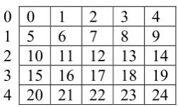
would be 5: 25, such that for 5 communications of cells, 25 cells are computed.
[image:38.595.271.397.565.641.2]0 0 1 2 3 4 1 5 6 7 8 9 2 10 11 12 13 14 3 15 16 17 18 19 4 20 21 22 23 24
Figure 3: A example of a 5x5 block with numbered cells
Clearly, this is preferable to a ratio of 3: 1 for the naïve parallel approach; but as it requires a pUnit to store the results of the final
30 column for the previously computed block ( 1) in all cases except for the first block in a row of blocks , further logic is necessary to achieve
this particular ratio. Note that if the cached column was not available,
the ratio would be increased to 11: 25, which is a result of having to communicate the details of the previous block 1 to the current block
. It would also be necessary to communicate the value of the final cell
of the block immediately to the north-west of . Striping is the requisite
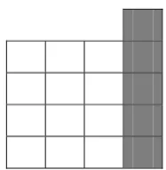
logic that allows for the caching of a column to serve as input to the next block. This logic sounds slightly off, but is redeemable if the cached
[image:39.595.292.386.334.430.2]column is of size 1, where denotes the height of an individual block in cells.
Figure 4: A 4x4 block with logical cached column highlighted13
It is important to note that when a pUnit processes a particular stripe,
any block is always dependent on its neighbouring block 1. If this ordering is violated, the produced alignment will be incorrect, or in the worst case, the program cannot run to completion. The use of stripes as
a mechanism for improving timeliness rests on the concept that given
stripes over some table and the set of pUnits , each pUnit will
be allocated some stripe where the range of is 0 to 1. In instances where the number of stripes is the size of , this mechanism is
trivial: each receives its own . Logically, this means in terms of
computation that in all cases excepting where 0 (for the first stripe to be computed) that is dependent on input from 1, which
13 The implementation does not make any attempt to store such a peculiar data structure; rather, it stores a
31 corresponds to (the previous stripe). The dependency in this case is
a block-level dependency; if a pUnit were required to wait for the composition of an entire stripe before performing its own tasks, there would be a surfeit of available processing time that would be wasted. Hence the segmentation of a stripe into blocks; at any stage, a pUnit
undertaking the composition of some block in some stripe requires
[image:40.595.318.431.253.347.2]the final row of the preceding block vertically in the table, .
Figure 5: Input row from a 5x5 block
This means that any is always going to be dependent on which
suggests that there is a threshold upon which no further speedup can be
gained, a threshold that is logically based upon the processing of blocks in a stripe, and physically based upon the maximum possible rate at which a pUnit can complete a block. The speedup for the parallel algorithm is discussed in the following section.
3.2.1.4 Speedup of the exact algorithm.
As stated in section 2.2.2.2, the speedup factor for a particular parallel algorithm over its sequential counterpart is formalised thus;
Where there is a tacit assumption that given a maximum factor , it is
always the case that , but that in certain circumstances . The results section details the actual results that were achieved through experimentation on different types of input data. Here, the theoretical
speedup of the parallel algorithm is described. Therefore, let denote
the sequential computation time over some table and denote the
32 And that,
.
Such that denotes the number of cells in . Section 2.4.2 describes
how can be calculated; essentially, it is the product of the number of
characters in a sequence from both alignment and alignment . More
simply assuming denotes a sequence from alignment and denotes a
sequence from alignment :
.
Where determines the number of characters in a given sequence.
This reasoning follows the original definition of the exact algorithm in
Kececioglu and Starrett’s (2004) paper in that the complexity of
generation of the dynamic programming table is a function of the number
of columns in the input alignments and , rather than the number of sequences in each alignment. To calculate the speedup for the parallel
algorithm, there are two factors that must be considered: first, the sum of
the communication penalties (see section 2.2.2.2) on all processors:
…
Where represents the total communication penalty over all pUnits,
denotes a logical pUnit from the set of pUnits and has the range 0 to where is the size of . Within the expression of is the term
which denotes the time of communication between processing units. To
calculate , it is necessary to introduce the second factor that must be
considered in the parallel speedup; a wait-factor that scales linearly
with . This wait-factor is a function of several elements of the parallel
algorithm; the processing of blocks, the number of pUnits , the number
of blocks in a stripe, and the number of stripes in the table .
Therefore, let denote the time to compute a single block;