Large Bayesian VARMAs

D

EPARTMENT OF

E

CONOMICS

U

NIVERSITY OF

S

TRATHCLYDE

G

LASGOW

LARGE BAYESIAN VARMAS

B

Y

JOSHUA C C CHAN, ERIC EISENSTAT AND GARY KOOP

N

O

14-09

S

TRATHCLYDE

Large Bayesian VARMAs

∗

Joshua C.C. Chan

Australian National University

Eric Eisenstat

University of Bucharest

Gary Koop

University of Strathclyde

September 25, 2014

Abstract: Vector Autoregressive Moving Average (VARMA) models have many the-oretical properties which should make them popular among empirical macroeconomists. However, they are rarely used in practice due to over-parameterization concerns, difficul-ties in ensuring identification and computational challenges. With the growing interest in multivariate time series models of high dimension, these problems with VARMAs become even more acute, accounting for the dominance of VARs in this field. In this paper, we develop a Bayesian approach for inference in VARMAs which surmounts these problems. It jointly ensures identification and parsimony in the context of an efficient Markov chain Monte Carlo (MCMC) algorithm. We use this approach in a macroeconomic application involving up to twelve dependent variables. We find our algorithm to work successfully and provide insights beyond those provided by VARs.

Keywords: VARMA identification, Markov Chain Monte Carlo, Bayesian, stochastic search variable selection

JEL Classification: C11, C32, E37

∗_{Gary Koop is a Senior Fellow at the Rimini Center for Economic Analysis. Emails:}

1

Introduction

Vector autoregressions (VARs) have been extremely popular in empirical macroeconomics and other fields for several decades (e.g. beginning with early work such as Sims, 1980, Doan, Litterman and Sims, 1984 and Litterman, 1986 with recent examples being Ko-robilis, 2013 and Koop, 2014). Until recently, most of these VARs have involved only a few (e.g. two to seven) dependent variables. However, VARs involving tens or even hun-dreds of variables are increasingly popular (see, e.g., Banbura, Giannone and Reichlin, 2010, Carriero, Clark and Marcellino, 2011, Carriero, Kapetanios and Marcellino, 2009, Giannone, Lenza, Momferatou and Onorante, 2010 and Koop, 2013, and Gefang, 2014). Vector autoregressive moving average models (VARMAs) have enjoyed less popularity with empirical researchers despite the fact that theoretical macroeconomic models such as dynamic stochastic general equilibrium models (DSGEs) lead to VMA representations which may not be well approximated by VARs, especially parsimonious VARs with short lag lengths. Papers such as Cooley and Dwyer (1998) point out the limitations of the structural VAR (SVAR) framework and suggest VARMA models as often being more appropriate. For instance, Cooley and Dwyer (1998) conclude “While VARMA models involve additional estimation and identification issues, these complications do not justify systematically ignoring these moving average components, as in the SVAR approach.” There is, thus, a strong justification for the empirical macreconomist’s toolkit to include VARMAs.

VARs are commonly used for forecasting. But, for the forecaster, too, there are strong reasons to be interested in VARMAs. The univariate literature contains numerous examples in finance and macroeconomics where adding MA components to AR models improves forecasting (e.g. Chan, 2013). But even with multivariate macroeconomic forecasting some papers (e.g. Athanasopoulos and Vahid, 2008) have found that VARMAs forecast better than VARs. Theoretical econometric papers such as Lutkepohl and Poskitt (1996) also point out further advantages of VARMAs over VARs.

Despite these advantages of VARMA models, they are rarely used in practice. There are three main reasons for this. First, there are difficult identification problems to be overcome. Second, VARMAs are parameter rich models which can be over-parameterized (an especially important concern in light of the growing interest in large dimensional models as is evinced in the growing large VAR literature). And, largely due to the first two problems, they can be difficult to estimate. This paper develops methods for estimating VARMAs which address all these concerns.

parameters and impulse responses that are more reasonable and estimated more accu-rately than alternative approaches, especially in the larger VARMAs of interest in modern macroeconomics.

2

The Econometrics of VARMAs

2.1

The Semi-structural VARMA

Consider the n dimensional multivariate time series yt, t = −∞, . . . ,∞ and begin with

the semi-structural form of the VARMA(p, q):

B0yt= p

X

j=1

Bjyt−j+ q

X

j=1

Θjǫt−j +Θ0ǫt, ǫt∼ N(0,Σ) (1)

or, in terms of matrix polynomial lag operators,

B(L)yt =Θ(L)ǫt,

and assume stationarity and invertibility. For future reference, denote the elements of

the VAR and VMA parts of the model as B(L) = [βki(L)] and Θ(L) = [θki(L)] for

i, k = 1, .., n.

The theoretical motivation for the VARMA arises from the Wold decomposition:

yt =K(L)ǫt, (2)

where K(L) is generally an infinite degree polynomial operator. Specifically, it can be

shown that any such rational transfer functionK(L) corresponds to the existence of two

finite degree operators B(L) and Θ(L) such that

B(L)K(L) =Θ(L).

Thus, the VARMA(p, q) is an exact finite-order representation of any multivariate system

that can be characterized by a rational transfer function. When K(L) is not rational, the

VARMA(p, q) can provide an arbitrarily close approximation. Moreover, an important

advantage of the VARMA class is that, unlike VARs or pure VMAs, it is closed under a

variety of transformations on yt, including linear operations and subsets.

The practical problem in having both AR terms with MA terms, however, is that an

alternative VARMA with coefficients B†(L) = C(L)B(L) and Θ†(L) = C(L)Θ(L) will

lead to the same Wold representation. The VARMA(p, q) representation, therefore, is in

general not unique. However, there are two reasons why a unique representation is desir-able in practice: parsimony and identification. The first reason concerns both frequentist

and Bayesian approaches. If B(L) and Θ(L) contain redundancies, then the resulting

B0 = Θ0 = I leaves 1,242 parameters (including error covariances) to estimate. With

macroeconomic data sets containing a few hundred observations, it will be very hard to obtain precise inference for all these parameters in the absence of an econometric method which ensures parsimony or shrinkage.

The second reason (lack of identification) may be less important for the Bayesian who is only interested in forecasting or in identified functions of the parameters such as impulse responses. That is, given a proper prior a well-defined posterior will exist even in a non-identified VARMA. However, the role of the prior becomes important in such cases and carelessly constructed priors can lead to deficient inference for the Bayesian. For frequentists, however, a lack of identification is a more substantive problem, precluding estimation.

How does one obtain a unique VARMA representation? There are generally two major steps:

The first step is to eliminate common roots in B(L),Θ(L) such that only C(L) with

a constant determinant is possible. In this case, the operators B(L),Θ(L) are said to

be left coprime and C(L) unimodular. For the univariate case, it is sufficient to achieve

uniqueness and corresponds in practical terms to specifying minimal orders p, q. For a

multivariate process, however, this is not enough and a second step is required. That

is, even if we impose B0 = Θ0 = I, there may still exist C(L) 6= I that preserves this

restriction for an alternative set of left coprime operators B†(L),Θ†(L). A common

example is

C(L) =

1 c(L)

0 1

.

Clearly, detC(L) = 1 and for any B(L),Θ(L), the transformations B†(L) = C(L)B(L)

and Θ†(L) =C(L)Θ(L) lead to B†₀ =Θ†₀ = I.

This implies that the elements of B(L),Θ(L) are not identified for estimation

pur-poses. One approach to achieving identification relies on the assumption that the matrix

[Bp : Θq] has full row rank, and indeed, when this holds then B0 = Θ0 = I induces a

unique representation (e.g., Hannan, 1976). In practice, one could try to explicitly

en-force [Bp :Θq] to have full row rank, but that may not be desirable in many applications.

The full row rank condition will likely not be satisfied by most data generating processes

(DGPs) in practice (L¨utkepohl and Poskitt, 1996). Therefore, forcing it in an estimation

routine would likely result in mis-specification and an alternative second step would be

required to achieve uniqueness when [Bp :Θq] is rank deficient.

The more general approach that we follow involves imposing exclusion restrictions on

elements of B(L),Θ(L) such that onlyC(L) = I is possible. It turns out that when such

zero restrictions are applied according to a specific set of rules, it is possible to achieve a

unique VARMA representation corresponding to a particular rational K(L). This leads

to the echelon form which we will use as a basis for our approach to identification.

2.2

The Echelon Form for the VARMA

every K(L) in (2) is associated with a unique set of indices κ= (κ1, . . . , κn), which can

be directly related to the VARMA operators B(L),Θ(L). Identification is achieved by

imposing restrictions on the VARMA coefficients in (1) according to so-called Kronecker indices κ1, . . . , κn, with 0≤κi ≤p∗, where p∗ = max{p, q}.

To explain further the identifying restrictions in the echelon form note that,

with-out loss of generality, we can denote the VARMA(p, q) as VARMA(p∗_{, p}∗_{). Then any}

VARMA(p∗_{, p}∗_{) can be represented in echelon form by setting B}

0 =Θ0 to be lower

tri-angular with ones on the diagonal and applying the exclusion restrictions defined by κ

to B₀, . . . ,Bp∗,Θ₁, . . . ,Θ_p∗. The latter restrictions impose on [B(L) : Θ(L)] a maximal

degree of each rowiequivalent toκi. A VARMA in echelon form is denoted VARMAE(κ)

and details regarding the foregoing restrictions are discussed in many places. The key

theoretical advantage of the echelon form is that, given κ, it provides a way of

con-structing a parsimonious VARMA representation foryt. A by-product of this is that the

unrestricted parameters are identified. At the same time, every conceivable VARMA can be represented in echelon form. The formal definition of the echelon form is given, e.g., in Lutkepohl, 2005, page 453 as:

Definition:

The VARMA representation in (1) is in echelon form if the VAR and VMA operators are left coprime and satisfy the following conditions.

The VAR operator is restricted as (for k, i= 1, . . . , n):

βkk(L) = 1−

Ppk

j=1βkk,jLjfor k = 1, . . . , n

βki(L) = −Pp_j=k_pk−pki+1βik,jLj for k 6=i ,

where

pki =

min(pk+ 1, pi) for k ≥i

min(pk, pi) for k < i .

The VMA operator is restricted as (for k, i= 1, . . . , n):

θki(L) = pk

X

j=0

θki,jLj and Θ0 =B0.

The row degrees of each polynomial arep1, . . . , pn. In the echelon form the row degrees

are the Kronecker indices which we label κ1, . . . , κn.

We specify a distinction between row degrees (p1, . . . , pn) and Kronecker indices

(κ1, . . . , κn) since this plays a role in our MCMC algorithm. In this, at one stage we work

with a VARMA that simply has row degrees p1, . . . , pn, but is otherwise unrestricted.

That is, it does not impose the additional restrictions (defined through pki) required to

put the VARMA in echelon form.

As an example of the echelon form, consider a bivariate VARMA(1,1), denoted as

y1,t

y2,t

=

β11 β12

β21 β22

y1,t−1

y2,t−1

+

θ11 θ12

θ21 θ22

ǫ1,t−1

ǫ2,t−1

+

ǫ1,t

ǫ2,t

. (3)

If it is known that β21 = β22 = θ21 = θ22 = 0, then y2,t =ǫ2,t and β12 is not separately

β12 = 0 orθ12= 0. However, knowing that y2,t =ǫ2,t implies that the Kronecker indices

of the system are κ1 = 1, κ2 = 0. Converting (3) to a VARMAE(1,0) yields

1 0

β0 1

y1,t

y2,t

=

β11 0

0 0

y1,t−1

y2,t−1

+

θ11 θ12

0 0

ǫ1,t−1

ǫ2,t−1

+

1 0

β0 1

ǫ1,t

ǫ2,t

.

Therefore, the rules associated with the echelon form automatically impose the identifying

restriction β12= 0.

The key challenge of applying the echelon form methodology in practice is

specify-ing κ. After all, any unrestricted VARMA is also a VARMAE for a particular set of

Kronecker indices. The problem is that whenever a particular κi is over-specified, the

resulting VARMAE is unidentified; whenever it is under-specified, the VARMAE is

mis-specified. Therefore, to exploit the theoretical advantages that the VARMAE provides,

the practitioner must choose the Kronecker indices correctly.

The standard frequentist approach to specifying and estimating VARMA models, in consequence, can be described as consisting of three steps:

1. estimate the Kronecker indices, ˆκ;

2. estimate model parameters of the VARMAE(ˆκ);

3. reduce the model (e.g. using hypothesis testing procedures to eliminate insignificant parameters).

It is important to emphasize that the order of the above steps is crucial. Specifically, step 2 cannot be reasonably performed without completing step 1 first. To appreciate the difficulties with implementing step 1, however, consider performing a full search procedure

over all possible Kronecker indices for an n-dimensional system. This would require

setting a maximum order κmax, estimating (κmax+ 1)n echelon form models implied by

each combination of Kronecker indices and then applying some model selection criterion

to select the optimal κ. Given the difficulties associated with maximizing a VARMAE

likelihood, even conditional on a perfectly specifiedκ, one cannot hope to complete such

a search in a reasonable amount of time (i.e. even a small system withn = 3 andκmax = 5

would require 1024 Full Information Maximum Likelihood (FIML) routines). Moreover,

many of the combinations ofκ1, . . . , κnthat a full search algorithm would need to traverse

inevitably result in unidentified specifications, thus plaguing the procedure with exactly the problem that it is designed to resolve.

To handle this difficulty, abbreviated search algorithms relying on approximations are typically employed. Poskitt (1992) provides one particularly popular approach. First, it takes advantage of some special features that arise if the Kronecker indices are re-ordered from smallest to largest such that the number of model evaluations is greatly reduced. Second, it involves a much simpler estimation routine for each evaluation step—i.e., a closed form procedure for consistently (though less efficiently than FIML) estimating the

free parameters of a VARMAE(κ). These two features also alleviate (although do not

However, the implementation also relies on a number of approximations. First, like all existing Kronecker search algorithms, Poskitt (1992) begins by estimating residuals from a long VAR. These are then treated as observations in subsequent least squares esti-mation routines, which are used to compute inforesti-mation criteria for models of alternative Kronecker structures. Based on the model comparison, the search algorithm terminates when a local optimum is reached. In small samples, therefore, the efficiency of this ap-proach will depend on a number of manual settings and may often lead to convergence difficulties in the likelihood maximization routines implemented at the second stage (for further discussion, see Lutkepohl and Poskitt, 1996).

Consequently, the procedure does not really overcome the basic hurdle: if the ˆκ

obtained in small samples incorrectly describes the underlying structure of the Kronecker

indices (as reliable as it may be asymptotically), the VARMAE(ˆκ) specified in step 2 may

ultimately be of little use in resolving the specification and identification issues associated with the unrestricted VARMA.

Recently, Dias and Kapetanios (2013) have developed a computationally-simpler iter-ated ordinary least squares (OLS) estimation procedure for estimating VARMAs. They prove its consistency and, although it is less efficient than the maximum likelihood es-timator (MLE), it has the advantage that it works in places where the MLE does not. In fact, the authors conclude (page 22) that “the constrained MLE algorithm is not a feasible alternative for medium and large datasets due to its computational demand.” For instance, they report that their Monte Carlo study which involved 200 artificial gener-ated data sets of 200 observations each from an 8 dimensional VARMA took almost one month of computer time. Their iterated OLS procedure is an approximate method, but the authors show its potential to work with larger VARMAs such as those considered in the present paper. However, their method does run into the problem that it can often fail to converge when either the sample size is small or the dimension of the VARMA is large. For instance, their various Monte Carlo exercises report failure to convergence rates from 79% to 97% for VARMAs with 10 dependent variables and T=150. These results are generated with VARMA(1,1) models and would, no doubt, worsen with longer lag lengths such as those considered in the present paper. These high failure to converge rates are likely due to the fact that, with many parameters to estimate and relatively little data to inform such estimates, likelihood functions (or approximations to them) can be quite flat and their optima difficult to find. This motivates one theme of our paper: use of carefully selected shrinkage through a Bayesian prior is useful in producing sensible (and computationally feasible) results in large VARMA models.

2.3

The Expanded Form for the VARMA

Papers such as Metaxoglou and Smith (2007) and Chan and Eisenstat (2014) adopt an alternative way of parameterizing the VARMA called the expanded VARMA form which proves useful for computational purposes. The expanded VARMA form, which provides an equivalent representation, can be written as:

B₀yt = p

X

j=1

Bjyt−j + p

X

j=0

Φjft−j +ηt, (4)

where ft ∼ N(0,Ω) and ηt ∼ N(0,Λ) are independent, Φ0 is a lower triangular matrix

with ones on the diagonal, Φ1, . . . ,Φp are coefficient matrices, and Ω,Λ are diagonal.

Since the parameters in the echelon form VARMA or the semi-structural VARMA can be recovered from the expanded VARMA parameters, it is clear that estimating the latter is sufficient to estimate the former. Our MCMC algorithm draws from the expanded VARMA form and then transforms draws to the echelon form.

Chan and Eisenstat (2014) provide an extensive discussion of the expanded VARMA form and its use in building MCMC algorithms. To summarize briefly, the expanded

form introduces n additional parameters, which are not fully identified even with the

echelon form restrictions imposed. However, this expansion of the parameter space does not require restrictive priors, nor does it impair sampling efficiency. In fact, because it leads to a straightforward linear state-space model, one can readily take advantage of a number of existing computational methods to construct fast sampling algorithms.

Moreover, working directly with the expanded form and transforming the draws ex post

to recover the original VARMA parameters circumvents the need to impose invertibility restrictions in the course of the MCMC. Instead, this is easily implemented in the ex

post processing of draws, i.e. in transforming Φ0, . . . ,Φq,Ω,Λ to Θ1, . . . ,Θq,Σ. A

straightforward algorithm for implementing the latter is detailed in Section 2 of Chan and Eisenstat (2014).

3

Bayesian Inference in VARMA Models

3.1

The Existing Bayesian Literature

Previously, we have drawn a distinction between the related concepts of parsimony and identification. Identification can be achieved by selecting the correct Kronecker indices (which imply certain restrictions on a semi-structural VARMA model). Parsimony is a more general concept, involving either setting coefficients to zero (or any constant) or shrinking them towards zero. So identification can be achieved through parsimony (i.e. selecting the precise restrictions implied by the Kronecker indices in the context of an unidentified VARMA model), but parsimony can involve imposing other restrictions on a non-identified model or imposing restrictions beyond that required for identifying the model.

Eisenstat (2014). The second consists of papers which explicitly address identification issues. The key references in this strand of the literature is Li and Tsay (1998). Since a key focus of our paper lies in identification, we will focus on this paper.

Li and Tsay (1998) specify a model similar to (1), i.e., with Θ0 lower triangular

but not equal to B0 and a diagonal Σ and work with the echelon form, attempting to

jointly estimate the VARMA parameters with the Kronecker indices (as we do in the present paper). This is done through the use of a hierarchical prior for the coefficients which is often called a stochastic search variable selection (SSVS) prior (although other terminologies exist). Before describing Li and Tsay’s algorithm, we briefly introduce the

idea underlying SSVS in a generic context. Let α be a parameter. SSVS specifies a

hierarchical prior (i.e. a prior expressed in terms of parameters which in turn have a prior of their own) which is a mixture of two Normal distributions:

α|γ ∼(1−γ)N(0, τ₀2) +γN(0, τ₁2), (5)

where γ is a dummy variable. Thus, ifγ = 1 then the prior for α is given by the second

Normal and if γ = 0 it is given by the first Normal. The prior is hierarchical since γ

is treated as an unknown parameter and estimated in a data-based fashion. The aspect which allows for prior shrinkage and variable selection arises by choosing the first prior variance,τ2

0, to be “small”(so that the coefficient is shrunk so as to be close to zero) and

the second prior variance, τ2

1, to be “large”(implying a relatively noninformative prior

for the corresponding coefficient). An SSVS prior of this sort, which we shall call “soft SSVS”, has been used by many researchers. For instance, George, Sun and Ni (2008) and Koop (2013) use it with VARs and Li and Tsay (1998) adopt something similar. An extreme case of the SSVS prior arises if the first Normal in (5) is replaced by a point mass at zero. This we will call “hard SSVS”. It was introduced in Kuo and Mallick (1997) and used with VARs by Korobilis (2013) and others.

Li and Tsay (1998) specify soft SSVS priors on the VAR and VMA coefficients of a VARMA. The ingenuity of this approach is that it combines in practical terms the two related concepts of identification and parsimony. The authors enforce the echelon form through this framework by imposing certain deterministic relationships between the SSVS indicators (see section 4 of Li and Tsay, 1998, for more details). Based on this,

they devise an MCMC algorithm that cycles through n individual (univariate) ARMAX

equations. The ith ARMAX equation is obtained by treating the observations {yj,t} for

j = 1, . . . , i −1, t = 1, . . . , T and the computed errors {ǫj,t} for j 6= i, t = 1, . . . , T

as exogenous regressors. SVSS indicators are then updated conditional on draws of the coefficients and subject to the deterministic relationships implied by the echelon form. In consequence, draws of the Kronecker indices (which can be recovered from draws of the SSVS indicators) are simultaneously generated along with the model parameters.

Their algorithm, however, entails a significant degree of complexity both in terms of programming and computation. A pass through each equation requires reconstructing VARMA errors (i.e. based on previous draws of parameters pertaining to other equations) and sampling three parameter blocks: (i) the autoregressive and “exogenous” variable coefficients, (ii) the error variance, and (iii) the moving average parameters. The latter

sweep of the MCMC routine. Evidently, the complexity of this algorithm grows rather

quickly with the size of the system, and in their applications, only systems with n = 3

and κmax ≤ 3 are considered. The run times reported for even these small systems are

measured in hours.

Relative to Li and Tsay (1998) our algorithm shares the advantage of jointly estimating Kronecker indices and model parameters, thus ensuring parsimony and identification. However, we argue that ours is a more natural specification, which also provides great computational benefits and allows us to work with the large Bayesian VARMAs of interest to empirical macroeconomists. First, by using the expanded form discussed in subsection 1.4, we are able to work with a familiar, linear state-space model. Conditional on the

Kronecker indices, computation is fast and efficient even for large n. Moreover, this

representation enables us to analytically integrate out the coefficients {Bj} and {Φj}

when sampling the Kronecker indices. The efficiency gains from this are particularly

important as n increases because the size of each Bj and Φj grows quadratically with n.

In fact, this added efficiency together with the reduced computational burden is precisely what allows us to estimate an exact echelon form VARMA for large systems. The details are provided in the following subsection.

Chan and Eisenstat (2014) develop an MCMC algorithm on the expanded form of the VARMA. However, it does not deal with identification using the echelon form as is done in the present paper. Nor does it deal with the challenges involved with large VARMAs (e.g. it does not develop shrinkage priors such as those we introduce shortly). Nevertheless, the MCMC algorithm developed in Chan and Eisenstat (2014) is the building block that we extend in the present paper when we derive an MCMC algorithm for the canonical echelon form.

3.2

Our Approach to Bayesian Inference in VARMAs

Our approach to Bayesian inference is based on the ideas that identification is achieved

in the echelon form (i.e. through estimating κ in the VARMAE(κ)), but computation

is more easily done in the VARMA(p, q) model in the expanded form (see also Chan

and Eisenstat, 2014). Thus, our MCMC algorithm works in the latter, but draws are

transformed to the echelon form. We also treatκas a vector of unknown parameters and

draw it in our algorithm. Parsimony and identification are achieved using SSVS priors.

In particular, we parameterize the echelon form by row degreesp1, . . . , pn and impose

two sets of restrictions: those implied by the row degrees and those resulting from the additional shrinking of model parameters. As will be made clear in this subsection, the echelon form is enforced by imposing a certain relationship between the two types of restrictions. All these elements are introduced in the model through a unified hierarchical SSVS prior.

Since row degree restrictions are especially important for identification, we always

use hard SSVS for these (i.e. the restrictions implied by a choice for p1, . . . , pn and,

thus, κ are imposed exactly). Restrictions on the remaining parameters are partly used

for identification and partly to achieve additional parsimony (i.e., by further restricting

parameters which remain in the VARMAE(κ)). For these, the researcher may wish to

terminology, we will call the prior which uses hard SSVS to achieve identification and soft SSVS to achieve parsimony the “soft SSVS prior” and the prior which imposes hard SSVS throughout the “hard SSVS prior”. In what follows, we describe the main features of our approach, paying particular attention to the SSVS priors on the VARMA coefficients. Complete details on the priors for the remaining parameters are given in Appendix A. Complete details of our MCMC algorithm are given in Appendix B.

Consider the expanded form VARMA given in (4) for which the VARMA coefficients

are parameterized in terms ofBi and Φi. Let the individual coefficients in these matrices

be denoted Bi,jk and Φi,jk, respectively. Here we describe the soft SSVS implementation

with τ2

0,ijk ≪ τ12,ijk (the hard SSVS implementation will be the same except there is no

τ2

0,ijk, but instead a point mass at zero is used) which is given by

Bi,jk|γ_ijkB,R, γ_ijkB,S

∼1−γ_ijkB,R1l(Bi,jk = 0)

+γ_ijkB,R1−γ_ijkB,SN(0, τ₀2,ijk) +γ B,S ijk N(0, τ

2 1,ijk)

,

Φi,jk|γijkΦ,R, γ

Φ,S ijk

∼1−γ_ijkΦ,R1l(Φi,jk = 0)

+γijkΦ,R

1−γijkΦ,S

N(0, τ02,ijk) +γ

Φ,S

ijk N(0, τ12,ijk)

, (6)

where 1l(·) is the indicator function. In this setup, γ_ijkB,R, γ_ijkΦ,R ∈ {0,1} are indicators determined completely by the row degrees: γ_ijkB,R =γ_ijkΦ,R = 1iff 0< j ≤ρiorj = 0, i < k.

Furthermore, γ_ijkB,S, γ_ijkΦ,S ∈ {0,1} are the indicators related to the SSVS mechanism for

the remaining coefficients not restricted by the row degrees.

Using the definition of the echelon form in subsection 1.3, define a mapping E(κ)

from the Kronecker indices to a set of indicators on the coefficients. We can use this

mapping in the construction of a set of restriction indicators for the echelon form: γE ₌

{γijkB,E, γ

Φ,E

ijk } = E(p1, . . . , pn). The echelon form can be imposed by specifying the prior

onγ_ijkB,S conditional on p1, . . . , pn as

Prγ_ijkB,S = 1|p1, . . . , pn

=

0 if γ_ijkB,E = 0, γ_ijkB,R 6= 0

0.5 otherwise . (7)

For the indicators on the elements of Φj we set Pr

γ_ijkΦ,S = 1 = 0.5.1 _{We further set}

uniform priors on p1, . . . , pn, which induce a prior on γR, and by implication, a uniform

prior on the Kronecker indices. Our MCMC algorithms provide draws of p1, . . . , pn,

and under the prior specification (7), these are equivalent to draws of the Kronecker

indices κ1, . . . , κn. Parameters of interest in terms of (1) can be recovered from draws

of B0,B1, . . . ,Bp, Φ0,Φ1, . . . ,Φp, Ω, and Λ using the procedure provided in Chan and

Eisenstat (2014).

A particular identification scheme can be imposed through a dogmatic prior which

sets probability one to a particular value for κ (e.g. allocating prior probability one to

1

κ1 = · · · = κn = p will be equivalent to estimating an unrestricted VARMA(p, p)). In

this case, we can work directly with γE _{(i.e. instead of γ}R_{) to enforce the echelon form}

restrictions, and the SSVS indicators γS _{= {γ}B,S

ijk , γ

Φ,S

ijk } would then be used exclusively

to control additional shrinkage: they can either be fixed a priori with P(γ_ijk·,S = 1) = 1

such that no additional shrinkage/variable selection is employed, or specified as _P(γ_ijk·,S =

1) = 0.5 and sampled in the course of the MCMC run along with the other parameters.

Applying the latter and naively setting κ1 =· · ·=κn =p leads to a simple SSVS model

where the parameters are potentially unidentified, but parsimony is achieved through shrinkage and computation is very fast.

Working with stochastic κ through stochastic row degrees p1, . . . , pn and indicators

γ_ijkB,S, γ_ijkΦ,S as outlined above, on the other hand, results in an algorithm that always

operates on a parameter space restricted according the echelon form, but also allows for additional shrinkage on the unrestricted coefficients. One interesting consequence of this is

that, unlike the classic VARMAE(κ) model in which the number of AR coefficients must

equal the number of MA coefficients, the additional SSVS priors allows the stochastic

search algorithm to uncover a VARMA(p, q) where p 6= q (i.e. if the SSVS mechanism

additionally forces certain coefficients to zero).

In sum, we argue that this SSVS prior can successfully address two of the three reasons (identification and parsimony) for a dearth of empirical work which uses VARMAs outlined in the introduction. The third reason was computation. Our MCMC algorithm, described in Appendix B, is fairly efficient and we have had success using it in quite large

VARMAs. For instance, we present empirical work below for VARMAs withn= 12 which

is much larger than anything we have found in the existing literature with the exception of Dias and Kapetanios (2013). However, dealing with much higher dimensional models

(e.g. n= 25 or more) as has been sometimes done with VARs would represent a serious,

possibly insurmountable computational burden, with our algorithm. Furthermore, real time forecasting exercises, requiring repeated MCMC estimation on an expanding window

of data, would pose challenges to our algorithm even with n= 12.

For these reasons, in Appendix B, we also describe an approximate MCMC algo-rithm which is much faster. This latter algoalgo-rithm is achieved by replacing (7), which involves prior dependencies between restrictions, with the simpler independent choice

Prγ_ijkB,S = 1 = 0.5. In our artificial data experiments (see below), this approximate

algorithm (which we call the “row degree algorithm”) seems to work quite well and is much more efficient than our exact algorithm (which we call the “echelon algorithm”). Complete details are given in Appendix B, but to understand the intuition underlying the approximate algorithm observe that (7) creates cross-equation relationships among

indicators, and therefore, strong dependence between the row degrees p1, . . . , pn. For

MCMC, this forces us to sample each pi conditional on all other row degrees and keep

track of all these relationships.

However, simplifying the prior on γ_ijkB,S as provided above allows the approximate row

practice, may be slight since the SSVS prior on the VARMA coefficients (i.e. involving

γS_{) should be able to pick up any restrictions missed by using an approximate algorithm.}

Thus, the row degree algorithm may be useful for the researcher who finds our echelon form algorithm too computationally demanding.

The MCMC algorithms described above can be used for selecting identifying restric-tions or deciding whether individual coefficients are zero or not. Of course, alternative methods of model comparison, involving marginal likelihoods or information criteria can be done using MCMC output. In our empirical section, we use the Deviance Information Criterion (DIC) for model comparison. Appendix C includes more details, including a definition and explanation of how we calculate it.

3.3

Extensions

In our empirical work, we use the models described in the preceding sub-section. However, we note that many extensions are possible. In this sub-section, we describe two directions which may be of use for the empirical macroeconomist. The first is to allow for a

time-varying Ωt or Σt. This can be done in a standard way by adding appropriate blocks to

the MCMC algorithm. For instance, multivariate stochastic volatility of the form used in Primiceri (2005) can be included by adding the extra blocks to the MCMC algorithm as described in Appendix A of his paper.

A second extension we consider is related to an alternative approach to analyzing

medium and large datasets. Specifically, let yt be an n×1 vector of dependent variables

that is categorized as follows:

• y₁,t: the n1 variables of primary interest;

• y2,t: then2 variables that together withytconstitute a fulln1+n2 variate VARMA

process;

• y3,t: the n3 additional variables that are used to identify factors ft.

Then, consider the following expanded form representation of the VARMA model:

yt= p

X

j=1

Bjyt−j + q

X

j=0

Φjft−j+ηt, ft∼ N(0,Ωt) and ηt ∼ N(0,Λ), (8)

where Φ1, . . . ,Φq are n ×n1 coefficient matrices and ft is n1 ×1. Consequently, the

covariance matrix Λ is of dimension n×n, whereas the time-varying covariance matrix

Ωt is diagonal with diagonal elements exp(h1,t), . . . ,exp(hn1,t), where the log-volatilities

follow a random walk process.

When n ≫ n1, (8) becomes a dynamic factor model, or under certain restrictions, a

4

Empirical Results

4.1

Artificial Data

In this section, we carry out a brief exercise with artificial data to investigate the perfor-mance of our algorithm. We focus on the identification issue and present results relating

toκ for various versions of our algorithm. All the results in this section involve drawing

10 artificial data sets, each of T = 100 observations. Each data set is normalized to

have mean zero and unit standard deviation. For each data set, 11,000 MCMC draws are taken and the first 1,000 of these discarded. All results are based on the benchmark prior described in Appendix A. We present results for the algorithm which imposes the echelon form exactly (labelled “echelon” in the tables below) versus the approximate algorithm which works with the row degrees (labelled “row degree” in the tables below). We also investigate the difference between the two different implementations of SSVS methods (labelled “hard SSVS” and “soft SSVS” in the tables) discussed in Section 2.

The first set of artificial data exercises uses bivariate VARMAs based on (3). Our first

data generating process (DGP) is a standard identified VARMA(1,1) with κ1 = κ2 = 1.

The second DGP is also a VARMA(1,1) but with κ1 = 1, κ2 = 0. In both cases, our

estimating model is an VARMA(4,4). The starting value forκ in the MCMC algorithm

is, throughout this section, always set so as to choose the VARMA(4,4). We are interested in investigating whether our algorithm can, in the context of a greatly over-parameterized model, uncover the parsimonious identified model in each case. Precise values of the parameters used in the DGPs are:

DGP1: β11 = 0.7, β21 = 0.4, β12 = 0.2, β22 = 0.5, θ11 = 0.1, θ12 = 0, θ21 = 0.5, θ22 =

0.1,Σ=

0.9 0

0 0.1

.

DGP2: β11= 0.7, β21 = 0, β12= 0.2, β22 = 0, θ11 = 0.1, θ12= 0, θ21= 0, θ22= 0.0,Σ=

0.9 0

0 0.1

.

Table 1 presents summary statistics of the various estimates of κ for the two DGPs.

It can be seen that, despite working with the over-parameterized VARMA(4,4), our

algo-rithm is accurately choosing the identified VARMAE(1,1) and VARMAE(1,0) for DGP1

and DGP2, respectively. The cross-data-set averages of κ do tend to be slightly above

the true values used in the DGP. In the case of κ2 in DGP2, this is of necessity (since

the true value ofκ2 = 0 and κ2 cannot be negative). For other cases, this is likely due to

excessively large lag length used in the estimating model. With regards to the different variants of our algorithms, there seems little difference. In particular, the approximate row degree algorithm is yielding results which are very similar to the exact algorithm which imposes the echelon form at every draw. Overall, though, the results indicate that our algorithms are working well in identifying small VARMAs. The estimates of the parameters (not reported here) are similar to the true values used in the DGPs and the inefficiency factors for the MCMC algorithm (also not reported here) indicate the algorithms are mixing well.

Table 1: Averages across Data Sets of Posterior Mean of κ. Standard Deviation, Mini-mum and MaxiMini-mum in Parentheses.

DGP1 DGP2

Algorithm details κ1 κ2 κ3 κ4

True value 1 1 1 0

echelon, 1.35 1.11 1.29 0.48

hard SSVS (0.19) (0.11) (0.06) (0.21)

(1.14, 1.68) (1.02, 1.40) (1.21, 1.36) (0.31, 0.99)

row degree, 1.28 1.24 1.59 0.49

hard SSVS (0.13) (0.15) (0.38) (0.21)

(1.18, 1.63) (1.14, 1.63) (1.31, 2.54) (0.32, 0.91)

echelon, 1.28 1.09 1.30 0.49

soft SSVS (0.25) (0.05) (0.21) (0.25)

(1.13, 1.93) (1.02, 1.17) (1.11, 1.85) (0.23, 1.05)

row degree, 1.23 1.20 1.32 0.42

soft SSVS (0.13) (0.14) (0.21) (0.30)

(1.12, 1.47) (1.12, 1.59) (1.14, 1.86) (0.25, 1.15)

in Tables 2 through 5. Tables 2 and 4 contain results relating to κ comparable to those

in Table 1 for larger 7-variate and 12-variate VARMAs. Tables 3 and 5 contain results relating to the efficiency of the MCMC algorithm. For the sake of brevity, inefficiency factors are presented for the impulse responses of the first and second variables to a shock

in the third variable four periods in the future. These are labelled “IR1” and “IR2” in

Tables 3 and 5.

The data generating process for the 7-variate VAR is a VARMA(1,1) with the following parameter values:

DGP3: B0 = Θ0 = I and βii = 0.1×i, θii = 0.1×(7 −i), β12 = β23 = −0.4,

θ56 = θ67 = −0.4 where βij and θij are the (i, j) elements of B1 and Θ1, respectively.

Letting σij be the elements of Σ, we set σii= 0.1×i, σ57 =σ67=−0.3. All elements of

B1, Θ1 and Σnot specified are set to zero.

Note that DGP3 has κi = 1 for i= 1, . . . ,7 and should be well-identified in the sense

that each row of the VARMA has either an AR or an MA coefficient which is substantively different from zero.

The data generating process from the 12-variate VAR is also a VARMA(1,1) with parameter values:

DGP4: B0 = Θ0 = I and βii = 0.1×i for i = 1, . . . ,8, θii = 0.1× (12− i) for

i= 1, . . . ,10,β12 =β23 =−0.4,θ56 =θ67 =−0.4 whereβij and θij are the (i, j) elements

of B1 and Θ1, respectively. Letting σij be the elements of Σ, we set σii = 0.1 ×i,

σ57=σ67=−0.3. All elements of B1, Θ1 and Σnot specified are set to zero.

Note that DGP4 has κi = 1 for i = 1, . . . ,10, with κ11 = κ12 = 0. However, for

equations 9 and 10 in the VARMA the identification is quite weak in the sense that both of these equations have no AR lags and the coefficient on the MA lag is quite small (i.e.

is quite close to the κ9 =κ10= 0 case.

Results for the medium-sized 7-variate VARMA are similar to those for the bivariate VARMA. Table 2 indicates the variants of our algorithm are all successfully producing

an estimate of κ near its true value. For none of the data sets do any of our algorithms

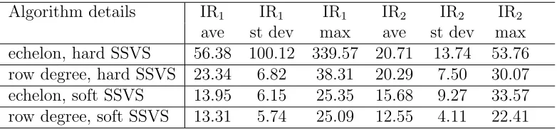
go far wrong. Table 3 indicates that the efficiency of our algorithm is fairly good, pro-ducing inefficiency factors that are around 10 or 20. However, the inefficiency factors for the echelon form algorithm with hard SSVS are somewhat higher than this. One of the artificial data sets leads to an inefficiency factor of over 300 for one of the impulse responses. Hence, the researcher using our algorithm in VARMAs of this size should take care with MCMC convergence issues and would probably be required to take hundreds

of thousands of draws,2 _{but MCMC convergence is unlikely to be a major worry. Indeed}

even the 10,000 draws (plus 1000 burn-in draws) used to produce the results in Table 2 appear to be enough to produce an accurate estimate of the true DGP in our artificial data exercise, despite the fact that the initial conditions used in our MCMC algorithm (based on the VARMA(4,4)) are far from the true VARMA(1,1).

Table 2: Averages across Data Sets of Posterior Pean ofκfor DGP3. Standard Deviations

in Parentheses.

Algorithm details κ1 κ2 κ3 κ4 κ5 κ6 κ7

True value 1 1 1 1 1 1 1

echelon, 1.05 1.01 1.01 1.04 1.07 1.00 0.90

hard SSVS (0.10) (0.01) (0.01) (0.09) (0.13) (0.01) (0.32)

row degree, 1.07 1.04 1.02 1.05 1.03 1.03 0.80

hard SSVS (0.10) (0.05) (0.03) (0.13) (0.03) (0.04) (0.34)

echelon, 1.01 1.02 1.01 0.99 1.03 1.01 0.80

soft SSVS (0.02) (0.05) (0.01) (0.08) (0.06) (0.01) (0.42)

row degree, 1.04 1.04 1.00 0.99 1.04 1.02 0.73

soft SSVS (0.05) (0.06) (0.03) (0.08) (0.05) (0.02) (0.43)

Table 3: Inefficiency Factors for Impulse Responses for DGP3.

Algorithm details IR1 IR1 IR1 IR2 IR2 IR2

ave st dev max ave st dev max

echelon, hard SSVS 56.38 100.12 339.57 20.71 13.74 53.76

row degree, hard SSVS 23.34 6.82 38.31 20.29 7.50 30.07

echelon, soft SSVS 13.95 6.15 25.35 15.68 9.27 33.57

row degree, soft SSVS 13.31 5.74 25.09 12.55 4.11 22.41

Results for the 12-variate VARMA are also quite encouraging. In Table 4, the

es-timates for κ1, . . . , κn are almost always very close to the true values in the DGP. The

only exception is for κ9 and κ10. But for the reasons noted previously, these are not

2

surprising. The four variants of the algorithm are producing similar results, although it is worth noting that the approximate row degree algorithms are producing estimates for

κ7 which are somewhat below those for the exact echelon algorithms.

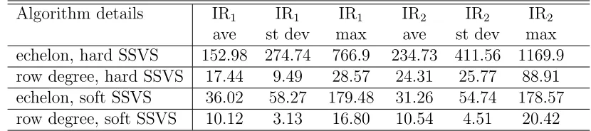
Table 5 presents evidence on MCMC efficiency. As expected, MCMC efficiency de-teriorates somewhat in this larger VARMA, but the row degree algorithm mixes much better than the echelon form algorithm. Of course, an exact algorithm is always to be preferred to an approximate one and, hence, where computationally possible we would recommend using the echelon form algorithm. However, Table 5 indicates that in larger VARMAs, the echelon form algorithm might be excessively computationally daunting or even infeasible in a reasonable amount of time. For instance, when using the echelon form algorithm with hard SSVS, one of our artificial data sets produces an inefficiency factor of over 1000 for estimation of one of the impulse responses suggesting that millions of draws may be required in some applications with larger VARMAs. In such applications, our approximate row degree algorithm, which is quite efficient even in the 12-variate VARMA, may be a good alternative.

It is also worth noting that MCMC algorithms using soft SSVS are much more efficient than hard SSVS. Even in the 12-variate VARMA, the echelon form algorithm with soft SSVS is producing inefficiency factors that are consistent with the researcher using tens (or at most a few hundred) of thousands of draws.

Table 4: Averages across Data Sets of Posterior Mean ofκfor DGP4. Standard Deviations

in Parentheses.

Algorithm details κ1 κ2 κ3 κ4 κ5 κ6

True value 1 1 1 1 1 1

echelon, 1.05 1.09 0.91 0.99 1.24 1.24

hard SSVS (0.11) (0.18) (0.23) (0.01) (0.31) (0.41)

row degree, 1.02 1.00 0.71 0.98 0.94 1.00

hard SSVS (0.06) (0.01) (0.42) (0.04) (0.23) (0.00)

echelon, 0.99 1.00 0.79 0.95 1.18 1.02

soft SSVS (0.01) (0.00) (0.36) (0.14) (0.39) (0.03)

row degree, 0.99 1.00 0.67 0.96 0.92 1.00

soft SSVS (0.01) (0.00) (0.44) (0.11) (0.23) (0.00)

κ7 κ8 κ9 κ10 κ11 κ12

True value 1 1 1 1 0 0

echelon, 1.00 0.96 0.04 0.02 0.00 0.00

hard SSVS (0.00) (0.12) (0.01) (0.03) (0.00) (0.00)

row degree, 0.33 0.98 0.03 0.02 0.00 0.00

hard SSVS (0.39) (0.05) (0.06) (0.02) (0.00) (0.00)

echelon, 0.81 0.93 0.01 0.01 0.01 0.00

soft SSVS (0.41) (0.16) (0.01) (0.01) (0.00) (0.00)

row degree, 0.21 0.94 0.01 0.01 0.00 0.00

Table 5: Inefficiency Factors for Impulse Responses for DGP4.

Algorithm details IR1 IR1 IR1 IR2 IR2 IR2

ave st dev max ave st dev max

echelon, hard SSVS 152.98 274.74 766.9 234.73 411.56 1169.9

row degree, hard SSVS 17.44 9.49 28.57 24.31 25.77 88.91

echelon, soft SSVS 36.02 58.27 179.48 31.26 54.74 178.57

row degree, soft SSVS 10.12 3.13 16.80 10.54 4.51 20.42

In summary, our artificial data exercise shows that our approach performs well in picking out the correct restrictions required to choose a correctly-identified parsimonious VARMA in the context of estimating an unidentified over-parameterized VARMA(4,4)

even whenn is quite large. The findings also lead us to recommend the use of soft SSVS

over hard SSVS for MCMC efficiency reasons and our empirical results using macroeco-nomic data will use soft SSVS. We also recommend the use of our exact echelon form algorithm as opposed to the approximate row degree algorithm where possible. But we in-clude the row degree algorithm in this paper since in larger VARMAs it may be required. Our empirical results using macroeconomic data use the echelon form algorithm.

4.2

Macroeconomic Application

In this section, we investigate the performance of our echelon algorithm (using soft SSVS and the prior specified in Appendix A) in a substantive empirical application involving

quarterly US macroeconomic data in VARMAs of varying dimensions: n= 3, n = 7 and

n= 12. We will draw all inference from a VARMA(4,4), of the form

yt =

4

X

j=1

Ajyt−j +

4

X

j=1

Θjǫt−j+ǫt, ǫt∼ N(0,Σ). (9)

For quarterly data, we conjecture that this is potentially over-parameterized. Therefore, for estimation purposes we will employ the echelon form and rely on the data to uncover the correct Kronecker structure. Our MCMC algorithms obtain draws directly from the expanded form. Upon the termination of the MCMC routine, however, we transform

all draws ex post to recover A1, . . . ,A4, Θ1, . . . ,Θ4, Σ in (9) above. We then analyze

estimates of these parameters and compute impulse responses. In sub-section 4.2.2 we also consider a simpler approach that involves sampling from (9) without employing the echelon form, but only specifying SSVS shrinkage priors on the over-parameterized

VARMA(4,4). We compare the results obtained with both approaches, as well as those

generated by a VAR(4) with SSVS priors on the VAR coefficients.

orthogonal to all other shocks) and classify every other variable as either “slow-moving” or “fast-moving” relative to this. Variables are ordered as slow-moving, then the monetary policy instrument, then the fast-moving variables. We stress that our variables have been transformed (e.g. GDP is log differenced) and that impulse responses reported below are to these transformed variables. Exact definitions of the variables, their transformations and classifications are given in Appendix D.

4.2.1 Results for our Preferred Model

In this sub-section, we focus on our preferred approach, as described in the preceding

sub-section. We run the algorithm for 50,000 iterations (5,000 burn-in) for the n = 3

model, 200,000 iterations (20,000 burn-in) for the n = 7 model, and 1,000,000 iterations

(100,000 burn-in) for the n = 12 model. For each model, we then thin the chains to

obtain exactly 10,000 draws (e.g., for n= 3 we take every 5th draw, forn = 7 every 20th

draw and forn = 12 every 100th draw). In each case, we set κmax= 4.

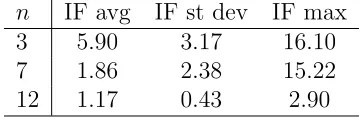
Figure 1 presents the estimated impulses responses of GDP, inflation and the interest rate to a shock in the interest rate, for 20 quarters following the shock. Table 6 presents inefficiency factors relating to these impulse responses. Specifically, it contains summary statistics for the inefficiency factors of the 60 different impulse responses computed and indicates that the number of draws taken is longer than necessary if one is only interested in obtaining impulse responses.

Table 6: Comparison of inefficiency factors for impulse responses across the three models:

n = 3, n = 7, and n = 12; note that the reported inefficiency factors are computed on

thinned draws.

n IF avg IF st dev IF max

3 5.90 3.17 16.10

7 1.86 2.38 15.22

12 1.17 0.43 2.90

Since we are interested in accurately estimating the Kronecker indices, we also present

results on MCMC performance relating to them. However, since κ1, . . . , κn are discrete

random variables, inefficiency factors are not an appropriate way to gauge sampling

ef-ficiency. In addition, any particular κi may naturally exhibit little movement over the

course of the sampler. For instance, if there is one correct choice for κi then a good

MCMC sampler would often (or even always) make such a choice and a lack of switching in the chain could be consistent with good MCMC performance. Accordingly, we shed light on the efficiency of the algorithm by the number of times the sampler switches

models, as defined by the entire vector κ. Specifically, we compute the metric

̟n =

G

X

g=1

1l n

X

i=1

κ(_ig)−κ_i(g−1)>0

!

/G,

where G is the number of MCMC draws, and consider that 10% represents sufficient

n= 3 n = 7 n = 12

0 5 10 15 20

−0.5 −0.4 −0.3 −0.2 −0.1 0 0.1 0.2

0 5 10 15 20

−0.5 −0.4 −0.3 −0.2 −0.1 0 0.1 0.2

0 5 10 15 20

−0.5 −0.4 −0.3 −0.2 −0.1 0 0.1 0.2

0 5 10 15 20

−0.3 −0.2 −0.1 0 0.1 0.2 0.3 0.4

0 5 10 15 20

−0.3 −0.2 −0.1 0 0.1 0.2 0.3 0.4

0 5 10 15 20

−0.3 −0.2 −0.1 0 0.1 0.2 0.3 0.4

0 5 10 15 20

−0.5 0 0.5 1

0 5 10 15 20

−0.5 0 0.5 1

0 5 10 15 20

−0.5 0 0.5 1

Figure 1: Impulse responses to a shock in the interest rate. The first row contains responses of GDP to a shock in the interest rate; the second row contains responses of inflation to a shock in the interest rate; the third row contains responses the interest rate

estimated κ for the VARMAs of different dimensions. Two general points are worth noting: the MCMC sampler is mixing well and the identification restrictions selected are much more parsimonious than the VARMA(4,4) estimating model. These facts suggest our modelling approach and associated MCMC algorithm are working well, even in large VARMAs.

A specific point worth noting is that, for output and inflation, the estimated Kronecker indices are consistent across VARMAs of different dimensions. In contrast, the Kronecker index for the interest rate decreases as the size of the system increases. This result is related to the ordering of the variables and is, in fact, consistent with the Kronecker

index theory. Loosely speaking, a Kronecker indexκi represents a threshold beyond which

autocovariances of further lags are linearly dependent on the lower-degree autocovariances

of variables 1, . . . , i. Since output and inflation are always ordered first, we expect that

the associated Kronecker indices do not change as additional variables are introduced. However, moving from three variables to seven, and especially from seven to twelve, introduces new variables that precede the interest rate. The fact that the Kronecker

index on the interest rate shrinks from an estimated ˆκ3 = 1.68 for the n = 3 system

to ˆκ9 = 0.01 for the n = 12 system indicates that the additional variables contain

all necessary information to explain the autocorrelations present in the interest rate.

In other words, we infer from the n = 12 system that the interest rate only responds

contemporaneously to slow moving variables; removing these variables from the model leads us to estimate the interest rate as an autocorrelated process.

Table 7: Comparison of estimated Kronecker indices across the three models: n = 3,

n= 7, and n= 12

n = 3 n = 7 n = 12

1 Real Gross Domestic Product 2.05 1.99 2.00

2 Consumer Price Index: All Items 2.12 2.01 2.00

3 Real Personal Consumption Exp. 1.00

4 Housing Starts: Total 1.00

5 Average Hourly Earnings: Manuf. 3.00 3.00

6 Real Gross Private Domestic Invest. 1.00

7 All Employees: Total nonfarm 1.00

8 ISM Manuf.: PMI Composite Index 1.00

9 Effective Federal Funds Rate 1.68 0.99 0.01

10 S&P 500 Stock Price Index 1.00 0.84

11 M2 Money Stock 1.28 0.97

12 Spot Oil Price: West Texas Interm 0.88 0.40

̟n 23.8% 13.7% 13.4%

The preceding table suggests our methodology is successfully picking out parsimonious identified models. To investigate this issue more deeply, Tables 8-9 present estimates of

the autoregressive and moving average coefficients in then = 12 model. For comparison,

discarding the echelon restrictions, and setting q = 0. We then use the algorithm de-scribed in Section 2.

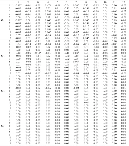
In Tables 8-9 it can be seen that the matrices of AR and MA coefficients are mostly zeros, particularly at longer lag lengths. This strengthens the evidence in support of our specification and algorithm successfully achieving parsimony. Note also that there are

several non-zero coefficients in Θ₁ (and some in Θ₂) indicating that adding MA terms

to the VAR is important. A careful examination of the MA coefficients shows that it is usually errors in the housing starts and the purchasing manager’s index equations that are found to be important. It is interesting to note that these two variables are typically regarded as leading indicators. Results for the housing starts variable are particularly interesting. When estimating the VARMA, we are finding in most equations that housing starts’ effect is best modelled through the MA part of the model. That is, other variables typically react to innovations in the housing starts equation, not lags of the housing starts

variable itself (i.e. the fourth columns of A1, . . . ,A4 are mostly zeros). Of course, the

VAR itself could not produce such a finding. It is interesting to note in Table 10 that lagged housing starts now appear much more prominently in the VAR part of the model, included in some equations at the second or third lag. This is as theory would predict. A parsimonious VARMA, such as that obtained in Tables 8-9, may be approximated by a VAR. However, the resulting VAR will be less parsimonious and with a longer lag length. In other words, it looks like the VAR(4) is trying to fit an inverted VARMA process.

4.2.2 Comparison with Alternative Approaches

In order to investigate the advantages of working with a VARMA over a VAR and the importance of imposing identification, in this sub-section we compare our preferred ap-proach to a different VARMA (which does have prior shrinkage but does not explicitly impose identification) and a VAR (which does have shrinkage but no MA components).

In particular, for each model of dimension n, we compare the following specifications:

• VARMAE(κ): our preferred echelon form VARMA with soft SSVS priors on AR

and MA coefficients and κmax = 4;

• VARMA(4,4): a VARMA with soft SSVS priors but no echelon form restrictions;

• VAR(4): a VAR with soft SSVS priors.

Note that we are only comparing modelling approaches which involve prior shrinkage. As we shall see below, empirical results such as impulse responses are clearly inferior and imprecise when we do not do have such shrinkage.

We begin by calculating DICs (see Appendix C) for each model and report the results

in Table 11. It can be seen that, for models of larger dimension, our VARMAE(κ) is

the preferred model by a substantial margin. Although when n= 3 the VARMA(4,4) is

preferred.

Each column in Table 11 contains results for a different value ofnand, thus, a different

yt. Hence, results are not comparable across columns and the table cannot be used to

Table 8: Posterior estimates of the moving average coefficients matrices Θ1, . . . ,Θ4 in a

VARMAE(κ). Note: * denotes that either Pr(θl,ij ≤0|y)≤0.1 or Pr(θl,ij>0|y)≤0.1;§ denotes

that either Pr(θ_{l,ij≤0|y)≤0}._{05 or Pr(}θ_l,ij>_0|y)≤0._{05;† denotes that either Pr(}θ_{l,ij≤0|y)≤0}.₀₁

or Pr(θ_l,ij>_0|y)≤0._01.

1 2 3 4 5 6 7 8 9 10 11 12

1 -0.19* -0.01 0.06 0.47§ _{-0.01 -0.04 0.20* 0.12 -0.02 0.06 0.00 -0.03}

2 -0.06 -0.08 0.07 0.03 0.01 -0.12 0.05 0.23§ _{0.03 0.01 0.01 0.04}

3 -0.09 -0.15 0.02 0.53§ _{0.00 0.04 -0.07 -0.12 -0.08 0.04 -0.03 -0.07}

4 -0.02 -0.01 0.01 0.08§ _{0.00 0.00 0.01 -0.01 -0.01 0.01 0.00 -0.01}

5 0.00 0.04 -0.05 0.17 0.01 -0.03 -0.03 0.05 -0.01 0.01 0.00 -0.01

Θ1 6 -0.20* 0.06 0.01 0.66† -0.03 -0.08 0.38† 0.20* 0.02 0.03 0.03 0.00

7 -0.08 -0.01 0.02 0.25§ _{-0.02 -0.04 0.03 0.13}§ _{-0.01 0.02 0.00 -0.01}

8 -0.07 -0.02 0.00 0.30† _{-0.01 -0.03 0.06 0.11* -0.02 0.02 0.01 -0.01}

9 -0.05 -0.02 0.01 0.15§ _{-0.01 -0.04 0.05 0.11}§ _{0.00 0.01 0.01 0.00}

10 -0.03 -0.03 0.01 0.26* 0.00 0.00 -0.07 -0.01 -0.04 0.06 0.01 -0.02

11 0.07 -0.02 0.00 -0.15 0.04 0.05 -0.12 -0.26§ _{-0.03 0.01 -0.09 -0.01}

12 -0.01 0.01 0.03 -0.11 0.00 -0.04 0.01 0.13* 0.01 0.01 0.02 0.03

1 -0.03 -0.03 -0.01 0.11 -0.01 -0.02 0.12 0.02 -0.04 -0.01 0.00 -0.01

2 0.04 -0.14 -0.02 -0.04 0.04 -0.01 -0.05 -0.11 -0.02 -0.02 -0.03 -0.09

3 -0.02 -0.02 0.00 0.07 -0.01 -0.01 0.08 0.01 -0.03 -0.01 0.00 -0.01

4 0.00 0.00 0.00 0.01 0.00 0.00 0.01 0.00 0.00 0.00 0.00 0.00

5 0.12 -0.05 -0.13* -0.01 -0.04 -0.11 0.24§ _{0.04 0.00 -0.01 0.00 0.00}

Θ2 6 -0.01 -0.02 -0.01 0.07 -0.01 -0.02 0.10 0.02 -0.03 -0.01 0.00 -0.01

7 0.00 -0.02 -0.01 0.03 0.00 -0.02 0.05 0.00 -0.01 -0.01 0.00 -0.01

8 0.01 -0.02 -0.02 0.02 -0.01 -0.02 0.06* 0.00 -0.01 0.00 0.00 -0.01

9 0.01 -0.03 -0.01 0.01 0.00 -0.01 0.01 -0.02 -0.01 -0.01 -0.01 -0.02

10 -0.02 0.00 0.01 0.03 0.00 0.00 0.01 0.00 -0.01 0.00 0.00 0.00

11 -0.02 0.07 0.01 0.01 -0.01 0.01 0.00 0.04 0.01 0.01 0.02 0.04

12 0.02 -0.03 0.00 -0.02 0.01 0.00 -0.03 -0.04 0.00 -0.01 -0.01 -0.02

1 0.00 0.00 0.00 0.00 0.00 0.00 0.00 0.00 0.00 0.00 0.00 0.00

2 0.00 0.00 0.00 0.00 0.00 0.00 0.00 0.00 0.00 0.00 0.00 0.00

3 0.00 0.00 0.00 0.00 0.00 0.00 0.00 0.00 0.00 0.00 0.00 0.00

4 0.00 0.00 0.00 0.00 0.00 0.00 0.00 0.00 0.00 0.00 0.00 0.00

5 -0.02 0.00 0.02 -0.05 -0.01 0.00 -0.02 0.08 0.00 0.01 0.01 0.01

Θ3 6 0.00 0.00 0.00 0.00 0.00 0.00 0.00 0.01 0.00 0.00 0.00 0.00

7 0.00 0.00 0.00 0.00 0.00 0.00 0.00 0.01 0.00 0.00 0.00 0.00

8 0.00 0.00 0.00 -0.01 0.00 0.00 0.00 0.01 0.00 0.00 0.00 0.00

9 0.00 0.00 0.00 0.00 0.00 0.00 0.00 0.00 0.00 0.00 0.00 0.00

10 0.00 0.00 0.00 0.00 0.00 0.00 0.00 -0.01 0.00 0.00 0.00 0.00

11 0.00 0.00 0.00 0.00 0.00 0.00 0.00 0.00 0.00 0.00 0.00 0.00

12 0.00 0.00 0.00 0.00 0.00 0.00 0.00 0.00 0.00 0.00 0.00 0.00

1 0.00 0.00 0.00 0.00 0.00 0.00 0.00 0.00 0.00 0.00 0.00 0.00

2 0.00 0.00 0.00 0.00 0.00 0.00 0.00 0.00 0.00 0.00 0.00 0.00

3 0.00 0.00 0.00 0.00 0.00 0.00 0.00 0.00 0.00 0.00 0.00 0.00

4 0.00 0.00 0.00 0.00 0.00 0.00 0.00 0.00 0.00 0.00 0.00 0.00

5 0.00 0.00 0.00 0.00 0.00 0.00 0.00 0.00 0.00 0.00 0.00 0.00

Θ4 6 0.00 0.00 0.00 0.00 0.00 0.00 0.00 0.00 0.00 0.00 0.00 0.00

7 0.00 0.00 0.00 0.00 0.00 0.00 0.00 0.00 0.00 0.00 0.00 0.00

8 0.00 0.00 0.00 0.00 0.00 0.00 0.00 0.00 0.00 0.00 0.00 0.00

9 0.00 0.00 0.00 0.00 0.00 0.00 0.00 0.00 0.00 0.00 0.00 0.00

10 0.00 0.00 0.00 0.00 0.00 0.00 0.00 0.00 0.00 0.00 0.00 0.00

11 0.00 0.00 0.00 0.00 0.00 0.00 0.00 0.00 0.00 0.00 0.00 0.00

Table 9: Posterior estimates of the autoregressive coefficients matrices A₁, . . . ,A₄ in a VARMAE(κ). Note: * denotes that either Pr(θl,ij ≤0|y)≤0.1 or Pr(θl,ij>0|y)≤0.1;§ denotes

that either Pr(θ_{l,ij≤0|y)≤0}._{05 or Pr(}θ_l,ij>_0|y)≤0._{05;† denotes that either Pr(}θ_{l,ij≤0|y)≤0}.₀₁

or Pr(θ_l,ij>_0|y)≤0._01.

1 2 3 4 5 6 7 8 9 10 11 12

1 0.01 -0.01 0.12* 0.08 0.06 0.01 0.07 0.09 -0.01 0.11* -0.02 -0.05

2 0.03 -0.54† _{0.04 0.01 0.01 0.00 0.01 0.12* 0.15}§ _{-0.02 0.02 0.08}

3 0.05 -0.05 0.03 0.12* 0.00 0.10 0.09 0.05 -0.15§ _{0.12* -0.07 0.00}

4 -0.04 0.03 0.04* 0.97† _{-0.01 0.06}§ _{0.01 -0.05}§ _-0.07† _{0.04* 0.01 0.00}

5 -0.01 0.03 -0.06 0.05 -0.80† _{-0.03 0.03 0.03 -0.02 0.03 0.01 0.02}

A1 6 -0.08 -0.02 0.29† -0.03 0.06 0.07 -0.07 0.12* 0.08 0.16§ -0.01 -0.03

7 -0.02 -0.08§ _0.11§ _{0.03 -0.02 0.02 0.67}† _0.11§ _{-0.02 0.12}† _{-0.03 0.03}

8 0.11* -0.02 0.07 0.05 -0.05* -0.03 -0.15§ _0.83† _-0.10§ _0.10§ _{-0.07* -0.01}

9 0.04 -0.10§ _{0.06* 0.05 0.00 -0.01 0.02 0.33}† _{-0.01 0.05}§ _{-0.02 0.01}

10 0.06 0.05 0.00 -0.01 0.10* 0.04 0.04 -0.28§ _{-0.05 0.19}§ _{-0.03 -0.02}

11 -0.09 -0.06 0.03 -0.02 -0.09 -0.10 0.04 0.03 -0.07 0.04 -0.15* 0.01

12 0.01 -0.05 -0.03 0.05 0.00 0.00 -0.02 0.09 0.02 0.00 -0.01 0.05

1 0.04 0.02 0.12* 0.00 -0.01 0.07 -0.06 0.01 -0.17† _{0.05 0.03 -0.04}

2 0.02 -0.22§ _{0.09 0.00 -0.01 -0.14}§ _{-0.02 0.05 0.02 -0.03 0.05 -0.10}

3 0.03 0.02 0.08* 0.00 -0.01 0.05 -0.04 0.00 -0.12† _{0.04 0.02 -0.02}

4 0.00 0.00 0.01* 0.00 0.00 0.01 -0.01 0.00 -0.02§ _{0.00 0.00 -0.01}

5 0.04 0.04 -0.04 0.02 -0.70† _{-0.02 0.07 0.01 -0.04 -0.03 -0.02 0.01}

A2 6 0.03 0.03 0.08* 0.00 -0.06 0.05 -0.04 0.00 -0.12† 0.04 0.02 -0.02

7 0.02 0.00 0.04* 0.00 -0.06§ _{0.01 -0.02 0.01 -0.06}§ _{0.01 0.01 -0.02}

8 0.02 0.00 0.03 0.00 -0.09† _{0.01 -0.01 0.01 -0.05}§ _{0.01 0.01 -0.01}

9 0.01 -0.03* 0.03* 0.00 -0.03 -0.02 -0.01 0.01 -0.02 0.00 0.01 -0.02

10 0.01 0.00 0.03* 0.00 0.05 0.02 -0.02 0.00 -0.04* 0.01 0.01 -0.01

11 -0.01 0.08§ _{-0.05 0.00 0.01 0.05* 0.01 -0.02 0.01 0.01 -0.03 0.04}

12 0.00 -0.08§ _{0.01 0.00 0.01 -0.05* 0.00 0.02 0.03 -0.02 0.01 -0.04}

1 0.00 0.00 0.00 0.00 0.00 0.00 0.00 0.00 0.00 0.00 0.00 0.00

2 0.00 0.00 0.00 0.00 0.00 0.00 0.00 0.00 0.00 0.00 0.00 0.00

3 0.00 0.00 0.00 0.00 0.00 0.00 0.00 0.00 0.00 0.00 0.00 0.00

4 0.00 0.00 0.00 0.00 0.00 0.00 0.00 0.00 0.00 0.00 0.00 0.00

5 0.00 -0.03 -0.08 0.01 -0.53† _{0.07 -0.01 -0.01 -0.07 0.05 0.09* 0.09*}

A3 6 0.00 0.00 -0.01 0.00 -0.04§ 0.01 0.00 0.00 -0.01 0.00 0.01* 0.01*

7 0.00 0.00 -0.01 0.00 -0.04† _{0.01 0.00 0.00 -0.01 0.00 0.01* 0.01*}

8 0.00 0.00 -0.01 0.00 -0.07† _{0.01 0.00 0.00 -0.01 0.01 0.01* 0.01*}

9 0.00 0.00 0.00 0.00 -0.02 0.00 0.00 0.00 0.00 0.00 0.00 0.00

10 0.00 0.00 0.01 0.00 0.04 -0.01 0.00 0.00 0.01 0.00 -0.01 -0.01

11 0.00 0.00 0.00 0.00 0.01 0.00 0.00 0.00 0.00 0.00 0.00 0.00

12 0.00 0.00 0.00 0.00 0.01 0.00 0.00 0.00 0.00 0.00 0.00 0.00

1 0.00 0.00 0.00 0.00 0.00 0.00 0.00 0.00 0.00 0.00 0.00 0.00

2 0.00 0.00 0.00 0.00 0.00 0.00 0.00 0.00 0.00 0.00 0.00 0.00

3 0.00 0.00 0.00 0.00 0.00 0.00 0.00 0.00 0.00 0.00 0.00 0.00

4 0.00 0.00 0.00 0.00 0.00 0.00 0.00 0.00 0.00 0.00 0.00 0.00

5 0.00 0.00 0.00 0.00 0.00 0.00 0.00 0.00 0.00 0.00 0.00 0.00

A4 6 0.00 0.00 0.00 0.00 0.00 0.00 0.00 0.00 0.00 0.00 0.00 0.00

7 0.00 0.00 0.00 0.00 0.00 0.00 0.00 0.00 0.00 0.00 0.00 0.00

8 0.00 0.00 0.00 0.00 0.00 0.00 0.00 0.00 0.00 0.00 0.00 0.00

9 0.00 0.00 0.00 0.00 0.00 0.00 0.00 0.00 0.00 0.00 0.00 0.00

10 0.00 0.00 0.00 0.00 0.00 0.00 0.00 0.00 0.00 0.00 0.00 0.00

11 0.00 0.00 0.00 0.00 0.00 0.00 0.00 0.00 0.00 0.00 0.00 0.00