Three-Layer Magnetoconvection

City, University of London Institutional Repository

Citation

:

Lin, M. K,, Silvers, L. J. and Proctor, M. R. E. (2008). Three-Layer

Magnetoconvection. Physics Letters A, 373(1), pp. 69-75. doi:

10.1016/j.physleta.2008.10.074

This is the unspecified version of the paper.

This version of the publication may differ from the final published

version.

Permanent repository link:

http://openaccess.city.ac.uk/1347/

Link to published version

:

http://dx.doi.org/10.1016/j.physleta.2008.10.074

Copyright and reuse:

City Research Online aims to make research

outputs of City, University of London available to a wider audience.

Copyright and Moral Rights remain with the author(s) and/or copyright

holders. URLs from City Research Online may be freely distributed and

linked to.

City Research Online:

http://openaccess.city.ac.uk/

publications@city.ac.uk

arXiv:0810.5279v2 [astro-ph] 29 Oct 2008

Three-layer magnetoconvection

M.-K. Lin

, L. J. Silvers

∗

, M. R. E. Proctor

a

Department of Applied Mathematics and Theoretical Physics, University of Cambridge, Cambridge, CB3 OWA, United Kingdom

b

St. Catharine’s College, University of Cambridge, Cambridge, CB2 1RL, United Kingdom

Abstract

It is believed that some stars have two or more convection zones in close proximity near to the stellar photosphere. These zones are separated by convectively stable regions that are relatively narrow. Due to the close proximity of these regions it is important to construct mathematical models to understand the transport and mixing of passive and dynamic quantities. One key quantity of interest is a magnetic field, a dynamic vector quantity, that can drastically alter the convectively driven flows, and have an important role in coupling the different layers. In this paper we present the first investigation into the effect of an imposed magnetic field in such a geometry. We focus our attention on the effect of field strength and show that, while there are some similarities with results for magnetic field evolution in a single layer, new and interesting phenomena are also present in a three layer system.

Key words: Magnetic Fields; Convection. PACS:44.25.+f; 47.65.-d.

1. Introduction

Throughout the Universe there are a plethora of stars with a variety of different internal structures[1]. Amongst the stars that we observe there are some, such as A-type stars, which are believed to have multiple convection zones near the surface [2,3], which is a phenomenon that results, to some extent, from the non-trivial changes in the chem-ical makeup as a function of distance centre of the star is increased [4]. The convection zones in these stars are thin, as compared to the radius of the star but are important as they affect the transport properties of this part of the star. As with all cases of convection in an astrophysical con-text, there are no solid boundaries encasing the convectively unstable fluid. Thus the ascending and descending plumes in the unstable regions can overshoot the convectively un-stable layer and continue into the adjacent convectively sta-ble region. Indeed, if the convection is sufficiently strong, or the adjacent stable region is sufficiently narrow, the over-shooting plumes can pass straight through the stable re-gion and enter the second convectively unstable rere-gion. It is thus clear that fascinating dynamical behaviour can be envisioned for this system and it is important to study such

∗ Corresponding author.

Email addresses:mkl23@cam.ac.uk(M.-K. Lin),

ljs53@damtp.cam.ac.uk (L. J. Silvers),mrep@damtp.cam.ac.uk (M. R. E. Proctor).

systems if we are to understand transport and mixing in stars where more than one convection zone is present.

Early analytical work on convection in stars with mul-tiple convection zones indicated that a separation of more than two pressure scale heights between the convection al-lows them to be considered as disjoint [4,6,7]. With ad-vances in computational resources, it has since become pos-sible carry out direct simulations of convection zones and their interaction with radiative zones, in application to so-lar convection or multiple convection zones in A-stars [5,8]. These simulations show the importance of further investi-gations into the mixing and transport in these stars as they demonstrate that a large degree of separation is required for the convection zones to be considered dynamically and thermally isolated[8].

The numerical investigations to date have been aimed at providing a solid basis for later, more complex, models. There are many further aspects of the physics of these stars which need to be considered and questions that still remain. Amongst these is the fact that convectively unstable regions in such stars are permeated by a magnetic field [10].

a scenario with multiple convection layers as described by Silvers & Proctor [8]. The purely hydrodynamic problem proved not to be a simple extension of single-layer systems, and we naturally anticipate at least the same complexity once a magnetic field is included. Exploring the effect of a magnetic field is also of interest because it has been con-jectured that certain chemical anomalies could result from magnetic fields in stellar atmospheres [10,16]. Michaud [17] suggested that field lines might stabilize the atmosphere to allow diffusion and guide particles into patches. It has also been suggested that magnetic fields may reduce the ion dif-fusion velocity [16].

In magnetoconvection calculations in a single unstable layer, the state that is reached after long times depends strongly on the strength of the magnetic field permeating the system. We expect to see a similar sensitivity here, and in addition we expect that the coupling between the layers is strongly affected by the field. Thus in the present paper we will explore the effect of varying field strength on the convection and interaction between two layers.

In this work we consider an atmosphere with two convec-tive zones separated by a stable layer with an initially ver-tical magnetic field. We do not address the specific problem of chemical anomalies by detailed modelling of stellar atmo-sphere composition and diffusion, as our goal is to provide a first understanding the effect of varying the strength of the magnetic field on convection through a simple model.

This paper is organised as follows: in the next section we describe our model with relevant equations, parameters and numerical method. In section 3 we present the results for cases with different strength magnetic fields. Finally, in section 4 we summarize our findings.

2. Model

We consider an atmosphere taking the form of a com-pressible fluid in a slab, with temperature decreasing piece-wise linearly with height, permeated by an imposed ver-tical magnetic field. The slab is comprised of three layers of equal thickness, the top and bottom being convectively unstable and the middle stable.

Apart from the multi-layer feature of the geometry, the equations are in standard form, as described in [8,13]. The governing equations are given in dimensionless form;

lengths are scaled by the depth d of each layer; density

and temperature byρ0 andT0, (values at z = 0, wherez

increases downwards); times by the sound crossing time

d/√R_∗T0whereR_∗ is the gas constant; and magnetic field

by B0, the magnitude of the initial uniform field. The

equations then take the form:

∂ρ

∂t +∇ ·(ρu) = 0 (1)

ρ _∂u

∂t +u· ∇u

=− ∇(P +F B2

/2) +θ(m+ 1)ρˆz

+∇ ·(FBB_+ρσκτ) (2)

∂T

∂t +u· ∇T+ (γ−1)T∇ ·u= γκ

ρ ∇

2

T

+κ(γ−1)(στ2

/2 +F ζ0J 2

/ρ) (3)

∂B

∂t =∇ ∧(u∧B−ζ0κ∇ ∧B) (4)

∇ ·B_{= 0 (5)}

P =ρT (6)

here F = B2

0/(R∗T0ρ0µ0), κ = K/(dρ0cp

√

R∗T0) the

dimensionless thermal diffusivity, τij ≡ ∂jui +∂iuj −

(2/3)δij∂kuk is the stress tensor andζ0 =ηcpρ0/K where

η is the magnetic diffusivity. Other quantities have their

usual meanings. The equations are solved using a mixed finite-difference/pseudospectral code. More details on the numerical method and code may be found in [13].

Through-out this paper we will use a resolution of 240×64×64.

For convenience we define the Chandrasekhar number

Q=F/ζ0σκ 2

, which provides a measure of field strength relative to diffusion and in what follows we will focus on the effect of varying this quantity, with other parameters held fixed. Their values are given in Table 1. Note that, for simplicity, we will introduce the notation that subscripts 1, 2 and 3 refer to respectively the top, middle and bottom zones. Also, we note here that our choice of polytropic

in-dices corresponds to the stiffness parameters S1 = S3 =

−1.0 for the top and bottom and S2 = 5.0 for the

mid-dle layer, whereS2 = (m2−mad)/(mad−m1) andS3 =

(m3−mad)(mad−m1); see e.g. [8].

Table 1

Parameter values.

Symbol Name Value

zm Vertical extent 3.0

ym=xm Horizontal extent 8.0

γ Ratio of specific heats 5/3

σ Prandtl number (=µcp/K, viscosityµ) 1.0

θ Temperature difference across a layer 10

ζ0 Magnetic diffusivity 0.2

m1=m3 Top and bottom polytropic index 1.0

m2 Middle polytropic index 4.0

R1 Rayleigh number near the top 5000.0

Q Chandrasekhar number variable

The initial three-layer structure, with different poly-tropic indices in the three layers is obtained by choosing a thermal conductivity profile of the form [8]:

K=K1 2

h

1 + K2+K3

K1 −

tanhz−1

∆

+K3

K1

tanhz−2

∆

−K_K2 1

tanh z−2

∆

tanh z−1

∆

i

(7)

where ∆ = 0.1 in this case, so as to allow a smooth transi-tion between the layers. To the static state we add random

velocity perturbations in the range [−0.05,0.05] and allow

the system to evolve. The boundary conditions at the top and bottom of the domain are taken to be:

T = 1, uz= ∂ux

∂z =Bx=By= ∂Bz

∂z = 0 atz= 0,

∂T

∂z =θ, uz= ∂ux

∂z =Bx=By= ∂Bz

∂z = 0 atz= 3, (8)

and all quantities are taken to be periodic inxandy with

periodsxm, ym.

3. Results

In this paper we explore the effect of varying magnetic

field strength, by varying the Chandrasekhar number, Q.

We begin with a discussion of the weak field case where

Q= 100. Figure 1 shows the distributions of vertical

mo-mentum density (ρuz, sides of the box) and of vertical

com-ponent of magnetic field (Bznear the top and bottom) once

the motion is fully established. This figure shows that the vertical magnetic field structure is dominated by regions of width between 0.4-0.7 between the convection cells in the upper layer. The lower layer does not resemble the upper layer, in spite of having the same polytropic index, because it has greater density and different values of other physical properties.

Fig. 1. Relative distribution of vertical component of magnetic field ( near the top and bottom) and vertical component of momentum (sides), for the caseQ= 100 att= 29.58.

The bottom field is relatively weak and much more uni-form, the most prominent structures being rising

conver-gent plumes (diameter≃0.9) with slightly enhanced values

ofBz. Distinct upflow and downflow regions can be seen in

the upper layer. In the central, stably stratified layer where

|ρuz|is small,Bzis almost uniform . The lower convection

zone, in contrast to the upper layer, has fewer and less or-dered convection cells, and there is little correlation with the field in the upper convection layer.

To explore the change in flows in more detail we

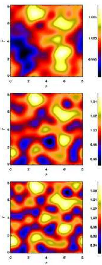
con-sider Figure 2 that shows horizontal slices ofBz and ρuz

Fig. 2. From top to bottom: vertical component of magnetic field (left) and vertical component of momentum (right) in the horizontal plane atz= 0.75,1.5,2.25; forQ= 100 andt= 29.58.

at the middle of each of the zones. At z = 0.75, regions

of high Bz corresponds to vertical motion, and from the

colourbar range on theρuzplot we see that downflows are

stronger, consistent with previous studies of compressible

magnetoconvection [12]. Regions of weakestBzmatches to

where|ρuz| ∼ 0 so any motion is in the horizontal plane.

This is again consistent with previous investigations, which showed that magnetic flux is swept by convection into con-verging regions within which the field is nearly parallel to

the fluid motion [11]. We also note that in theρuz plots,

there is little variation within the upflow cells.

In the convectively stable region, atz = 1.5, there is a

much smaller variationBz andρuzthan in the upper

con-vection zones. The pattern of motion is very weakly

corre-lated with that at atz= 0.75 forBz with rolls still

domi-nant but of larger widths (∼1 unit). The mid-layerρuzis

typically anti-correlated to the upper layer; for example the downflow region in the lower half of the plot corresponds

to upflow at z = 0.75, although the former is thinner in

extent. Comparing the plots we can see that vertical field

and motion atz = 0.5 are almost unrelated. It is

In the lower convection zone, atz= 2.25, the contrast in

Bzis similar to that in the central region but the pattern is

more cellular. Interestingly, although this layer is

convec-tively unstable, Bz does not correlate well to ρuz, unlike

in the top layer. The distribution ofρuz is almost uniform

with small cells (diameter ∼0.5 units) of strong upwards

motion and their positions appear unrelated. These slice

plots show distinct changes in Bz across the layers,

sug-gesting that for a weak field, its associated structure can not be easily communicated across boundaries, from this perspective the three layers appear independent. However, the boundary conditions on the interface allow overshoot-ing, which is another form of communication across bound-aries, and is best illustrated by considering the variation of

|ρuz|withz.

Fig. 5 shows snapshots ofh|ρuz|iandhB2ias a function

ofzfor theQ= 100 case, where angle brackets denote

hor-izontal averages. It is possible that such snapshots can be misleading as they can be contaminated by acoustic and gravity modes. However, we have verified by looking at other snapshots that the distributions of the two quantities shown are typical in the statistically steady state. As ex-pected vertical motion dominates in the two convectively unstable zones due to convection, but the solid lines extend from both unstable zones into the middle so there is non-zero vertical motion throughout the stable region which in-dicate overshooting. The motion in the upper convection zone is more vigorous and the solid curve extends into the mid-layer more than that from the lower convection zone, which suggests more overshooting from the upper layer into the middle. This is indeed consistent with the slice plots (Figure 2); but as we will show later, the correspondence is not universal. In the statistically steady state the top also contains most of the magnetic energy. The typical value of

hB2

iin the middle is∼0.37 times the maximum (in the

up-per layer) so some of the up-perturbation to magnetic energy ‘overflows’ into the middle. Although there is more motion in the lower zone than the middle there is not much field amplification, and from this together with the slice plots above we conclude that stronger motions are required to

increasehB2

iat the bottom, as seems very reasonable given

the greater density there.

Having discussed the weak field,Q= 100 case, we now

move to examine the effect of increasing the Chandrasekhar

number to Q = 500. As we have shown for the Q = 100

case, the motion is largely confined to the top and bottom

layers shown in Figure 3. Furthermore, for this Q = 500

case, near the top we notice hexagonal-type cells of size∼

1.6−1.8 dominate, the stronger field has reduced

horizon-tal scales because particle motion is more confined along field lines. The sides of the box also show that the con-vection cells in the upper layer are less prominent than for

Q = 100. The variation with z for the Q = 500 case is

shown more clearly in Fig. 4. At z = 0.75,Bz is

concen-trated in circular and triangular cells, corresponding to

up-flow and downup-flow regions in theρuzplot. These regions of

concentrated vertical flux are separated by rings with low

Fig. 3. Relative distribution of vertical component of magnetic field (near the top and bottom) and vertical momentum density (sides), for the caseQ= 500 att= 37.12.

Fig. 4. From top to bottom: vertical component of magnetic field (left) and vertical component of momentum (right) in the horizontal plane atz= 0.75,1.5,2.25; forQ= 500 andt= 37.12.

Bz, and correspond to regions of low|ρuz|. At this depth

there is strong correlation between field and motion; a

be-haviour that is similar toQ= 100 and is again consistent

with the general picture of one-layer magnetoconvection.

In the stable region, atz= 1.5, the associated disturbance

Fig. 5. Horizontal average of modulus of vertical momentum density (solid) and magnetic energy (solid line), as a function of depth, for

Q= 100 att= 29.58.

sible for weak fields) from one region into another. A typ-ical convection cell would require some horizontal motion but if this is opposed by a strong vertical field then par-ticles are more likely to continue in the vertical direction. However, we must also note that increasing field strength is to reduce motion, as discussed later, so in terms of over-shooting there is a competition between the two factors.

Fig. 4 shows the middle layer (z = 1.5) has generally

lower values ofBz and around half as much contrast than

atz= 0.75 because motion is less vigorous andρuzat this

depth is typically an order of magnitude smaller than at

z= 0.75. The figure shows no correlation betweenρuzand

Bz for the mid-layer, as with Q= 100. However, in

con-trast to the weak field case where there is some similarity

betweenρuzatz= 0.75,1.5; here the hexagonal structure

in the upper layer is entirely absent in the middle. Despite

the strong similarity inBz, information about vertical

mo-tion is not transported from the top to the middle. In fact,

comparingρuz atz= 1.5,2.25 show some correspondence

(see, for example, the roll [in red] near the top left of the two plots). This suggests the increased field may have reduced overshooting from top and increased it from the bottom. We conclude from Fig. 4 that, since there is no requirement

that Bz andρuzto be related in a convectively stable

re-gion, the middle may echo either of the structures above or below. In order to test whether the effect of increas-ing the Chandrasekhar number is to reduce overshootincreas-ing from the top and increase it from the bottom, we exam-ine once again, the modulus of the vertical component of momentum density shown in Fig. 6 to compare the three

regions. In conjunction with Fig. 5 (Q= 100), we see that

h|ρuz|iQ=100>h|ρuz|iQ=500so increased field has generally

suppressed convection. Although the plot for Q = 500 is

qualitatively very similar to that forQ= 100 the decrease

in max(h|ρuz|i) from Q= 100 toQ= 500 is 1.18→0.70

in the upper layer and 0.29→0.21 in the bottom layer and

thus activity in the top layer is more strongly suppressed. This implies that the extent of overshooting from the bot-tom relative to that from the top has increased with field

Fig. 6. Horizontal average of modulus of vertical momentum (solid line) and magnetic energy divided by F (dashed line), as a function of depth, forQ= 500 att= 37.12.

Fig. 7. Relative distribution of vertical component of magnetic field (near the top and bottom) and vertical component of momentum (sides), for the caseQ= 1000 att= 53.60.

strength. Although the top has more vigorous motion, for overshooting we must consider also the direction of motion,

and we will return to this when we considerhρuzilater. Fig.

6 shows that the variation ofhB2

i, in comparison to the

weak field case, is smaller but that the variation withzis

similar. The typical value at the middle is∼0.70 times the

maximum, which shows that stronger fields can increase the amount of magnetic energy pumped downwards, thereby transporting the structure and hence providing more con-nection. However, since the viogour of motion is suppressed

(compared toQ= 100) there is no increased overshooting

from the top.

We now move to discuss the Q = 1000 case for which

Fig. 7 shows an almost inverted distribution of structure

and activity compared with that for Q = 100 and Q =

500. The bottom has magnetic structure with a

horizon-tal scale comparable to that for the top of the Q = 500

case, although the distribution is less ordered. Convection

is predominantly in the bottom layer with typical size ∼

Fig. 8. From top to bottom: vertical component of magnetic field in the horizontal plane at z = 0.75,1.5,2.25; for Q = 1000 and

t= 53.60.

be almost featureless with an almost uniformBzand little

vertical motion. The slice plots shown in Fig. 8 confirm this

effect. This figure shows that the form ofBz atz= 0.75 is

different to that atz= 1.5,2.25 but the latter two plots are

similar; the disturbance toBzis now transported from the

bottom upwards, in contrast to the caseQ= 500. Although

the plots show rich structure, note that the contrast inBz

is only∼0.01,0.05,0.12 units forz= 0.75,1.5,2.25

respec-tively, and these are all smaller than for previous cases, so the field is almost unperturbed and remains mostly verti-cal. However, as for previous cases we found the strongest flow-field correlation for the layer with most magnetic

dis-turbance, which is the bottom layer for Q = 1000. This

continues the trend fromQ= 100→500, that

overshoot-ing from the bottom relative to the top has increased, and

Fig. 9. Horizontal average of modulus of vertical momentum (solid) and magnetic energy divided by F (dashed line), as a function of depth, forQ= 1000 att= 53.60.

is further supported by Fig. 9 that show vertical motion

al-most completely suppressed forz <1.7 buth|ρuz|iis still

comparable to previous cases in the lower convection zone. Since the top is suppressed, overshooting from the bottom

dominates; in facth|ρuz|iforz >2 is qualitatively similar

to the reverse of the curve in the top layer inQ= 100 and

Q= 500. A strong field resists deformation so there is only

a 1% perturbation tohB2

i. As before, the most vigorous

region (bottom layer here) contains most magnetic energy but unlike previous cases the middle has a significant por-tion of magnetic energy. These observapor-tions are again

dif-ferent from that forQ= 100,500. We have also done

cal-culations forQ = 1500; these show the same effect as for

Q= 1000 but to a greater degree, and forQ= 750, which

show features intermediate between theQ= 500 andQ=

1000 cases.

4. Conclusions

In this letter we have examined three-layer magneto-convection and we have focused on the effect of varying the strength of the magnetic field via varying the

Chan-drasekhar numberQ. For weak imposed magnetic field and

for our parameter choices convection occurs in both the top and bottom layers. For such fields the magnetic field behaves passively and is easily swept into the intracellular regions. As we increased the strength of the magnetic field we showed at the magnetic field forces substantial changes onto the flow. We showed that for modest strength

mag-netic field, e.g. for theQ = 500 case, the magnetic field

forces a fairly regular convection pattern in the upper layer. However, we showed that if the magnetic field becomes too

strong, as for example in theQ= 1000 case motion in the

which the unstable layers can communicate with each other through a stable region can be significantly affected by a magnetic field permeating all three layers. Further work at higher Rayleigh numbers is undoubtedly required to show whether the behaviour found persists in turbulent flows.

Acknowledgements

LJS & MREP wishes to thank STFC for the award of a rolling grant to fund research in magnetoconvection. MKL wishes to thank St. Catharine’s College for support for this project. We are grateful to Paul Bushby for helpful discus-sions.

References

[1] M. Schwarzschild, Structure and Evolution of Stars, Dover, New York, NY, 1965.

[2] J. D. Landstreet, Astron. Astrophys. 338 (1998) 1041.

[3] J. Silaj, A. Townsend, F. Kupka, J. Landstreet, A. Sigut, EAS Pub. Series, 17 (2005) 345.

[4] J. Toomre, J.-P. Zahn, J. Latour, E. A. Spiegel, Astrophys. J. 207 (1976) 545.

[5] H. J. Muthsam, W. Gob, F. Kupka, New Astronomy 4 (1999) 405.

[6] J. Latour, E. A. Spiegel, J. Toomre, J.-P. Zahn, Astrophys. J. 207 (1976) 233.

[7] J. Latour, J. Toomre, J.-P. Zahn, Astrophys. J. 248 (1981) 1081. [8] L. J. Silvers, M. R. E. Proctor, Mon. Not. R. Astron. Soc. (2007)

submitted

[9] G. Vauclair, S. Vauclair, G. Michaud, Astrophys. J. 223 (1978) 920.

[10] G. W. Preston, Ann. Rev. Astron. Astrophys. 12 (1974) 257. [11] N. O. Weiss, Proc. Roy. Soc. London A. 293 (1966) 316. [12] N. E. Hurlburt, J. Toomre, Astrophys. J. 327 (1988) 920. [13] P. C. Matthews, M. R. E. Proctor, N. O. Weiss, J. Fluid Mech.

305 (1995) 281.

[14] M. R. E. Proctor. Magnetoconvection. Invited review in: Fluid dynamics and dynamos in astrophysics and geophysics, ed. Soward, Jones, Hughes and Weiss, CRC Press, (2005) 235. [15a] S. M. Tobias, N. H. Brummell, T. L. Clune, J. Toomre,

Astrophys. J. Lett. 502 (1998) 177.

[15b] S. M. Tobias, N. H. Brummell, T. L. Clune, J. Toomre, Astrophs. J. 549 (2001) 1183.

[16] S. Vauclair, G. Vauclair, Ann. Rev. Astron. Astrophys. 20 (1982) 37.

[17] G. Michaud, Astrophys. J. 160 (1970) 641.

[18] E. F. Borra, J. D. Landstreet, Astrophys. J. Suppl. 42 (1980) 421.