City, University of London Institutional Repository
Citation:
Castro Alvaredo, O. & Fring, A. (2002). Conductance from Non-perturbative Methods II. Journal of High Energy Physics, 2002(10),This is the published version of the paper.
This version of the publication may differ from the final published
version.
Permanent repository link:
http://openaccess.city.ac.uk/16433/Link to published version:
Copyright and reuse: City Research Online aims to make research
outputs of City, University of London available to a wider audience.
Copyright and Moral Rights remain with the author(s) and/or copyright
holders. URLs from City Research Online may be freely distributed and
linked to.
City Research Online: http://openaccess.city.ac.uk/ [email protected]
arXiv:cond-mat/0210592v1 28 Oct 2002
PrHEP unesp2002
Conductance from Non-perturbative Methods II
Olalla A. Castro-Alvaredo∗ and Andreas Fring
Institut f¨ur Theoretische Physik, Freie Universit¨at Berlin, Arnimallee 14, D-14195 Berlin, Germany
E-mail: [email protected],[email protected]
Abstract: This talk provides a natural continuation of the talk presented by Andreas Fring in this conference. Part I was focused on explaining how the DC conductance for a free Fermion theory in the presence of different kinds of defects can be computed by evaluating the Kubo formula. In this talk I will focus on an alternative method for the computation of the same quantity, that is the evaluation of Landauer formula. Once again, the integrability of the theories under consideration will be exploited, since a ther-modynamic Bethe ansatz analysis provides all the input needed in that case, apart from the corresponding reflection and transmition amplitudes of the defect. The basic conclu-sion of our analysis will be the perfect agreement between the two different theoretical descriptions mentioned.
The results I will talk about are contained on a series of papers [1, 2, 3, 4, 5, 6], with emphasis on the first two, resulting mainly from a collaboration with Andreas Fring, who presented the first part of the work.
1. Thermodynamic Bethe ansatz for impurity systems
As mentioned in the previous talk, for the evaluation of the Landauer formula [7] one needs to know the density distribution functions involved. I will now present a general method which allows to compute such quantities non-perturbatively, i.e. the thermodynamic Bethe ansatz (TBA) approach, which we generalized in [1] to incorporate the non-trivial effects arising due to the presence of impurities. Besides the aim we have in mind, in general the TBA is a powerful tool for the computation of thermodynamic quantities in 1+1 dimen-sional integrable systems. Originally formulated by Yang and Yang [8] in the context of the non-relativistic Bose gas, it was thereafter generalized by Zamolodchikov [9] to relativis-tic quantum field theories which interact by means of factorizable scattering matrices. A TBA-analysis serves to check the consistency of a certain S-matrix proposal, since it allows
PrHEP unesp2002
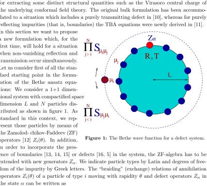
for extracting some distinct structural quantities such as the Virasoro central charge of the underlying conformal field theory. The original bulk formulation has been accommo-dated to a situation which includes a purely transmitting defect in [10], whereas for purely reflecting impurities (that is, boundaries) the TBA equations were newly derived in [11]. In this section we want to propose
S
000 000 000
111 111 111
000 000 000
111 111 111
00 00 00
11 11 11
Π
Π
S
L
α
Z
i j
i
j
j
j
i
j
R T
,
µ µ
µ µ
N
N > i
< i
[image:3.612.86.513.86.470.2]µ
µ
Figure 1: The Bethe wave function for a defect system.
a new formulation which, for the first time, will hold for a situation when non-vanishing reflection and transmission occur simultaneously. Let us consider first of all the stan-dard starting point in the formu-lation of the Bethe ansatz equa-tions: We consider a 1+1 dimen-sional system with compactified space dimension L and N particles dis-tributed as shown in figure 1. As standard in this context, we rep-resent those particles by means of the Zamolod- chikov-Faddeev (ZF) operators [12] Zi(θ). In addition,
in order to incorporate the
pres-ence of boundaries [13, 14, 15] or defects [16, 5] in the system, the ZF-algebra has to be extended with new generatorsZα. We indicate particle types by Latin and degrees of
free-dom of the impurity by Greek letters. The “braiding” (exchange) relations of annihilation operators Zi(θ) of a particle of type imoving with rapidity θ and defect operatorsZα in
the stateα can be written as
Zi(θ1)Zj(θ2) = Sijkl(θ1−θ2)Zk(θ2)Zl(θ1), (1.1)
Zi(θ1)Zj†(θ2) = Sijkl(θ1−θ2)Zk†(θ2)Zl(θ1) + 2πδ(θ1−θ2)δij, (1.2)
Zi(θ)Zα = Rjβiα(θ)Zj(−θ)Zβ+Tiαjβ(θ)ZβZj(θ), (1.3)
ZαZi(θ) = ˜Riαjβ(−θ)ZβZj(−θ) + ˜Tiαjβ(−θ)Zj(θ)Zβ. (1.4)
The bulk scattering matrix is indicated byS, and the left/right reflection and transmission amplitudes through the defect are denoted byR/R˜ and T /T˜, respectively as seen in part I. We employed Einstein’s sum convention, that is we assume sums over doubly occurring indices. We suppress the explicit mentioning of the dependence of Zα on the position
PrHEP unesp2002
convenience the following shorthand notation for the product of various particle operators
Zi(θ) and a defect operator Zα
Zµ1...µN
k,α :=Zµ1(θµ1). . . Zµk(θµk)ZαZµk+1(θµk+1). . . ZµN(θµN). (1.5)
Then we compute the braiding of a particle operator of type iand the previous product
Zµ1...µN
k,α by using the algebra (1.1)-(1.4) and assuming the S-matrix of the bulk theory to
be diagonal
Zi(θi)Zk,αµ1...µN = Zk,αµ1...µNZi(θi) ˜Fiα−Zk,αµ1...µNZi(−θi) ˜Giα, (1.6)
Zµ1...µN
k,α Zi(θi) = Zi(θi)Z
µ1...µN
k,α Fiα−Zi(−θi)Z
µ1...µN
k,α Giα. (1.7)
We abbreviated here
˜
Fiα= 1 ˜
Tα i (−θi)
N
Y
l=1
Siµl(θiµl), G˜
α
i =
˜
Rαi(−θi)
˜
Tα i (−θi)
k
Y
l=1
Siµl(θiµl)
N
Y
l=k+1
Siµl(−θˆiµl), (1.8)
Fiα= 1
Tα i (θi)
N
Y
l=1
Sµli(θµli), G
α
i =
Rαi(θi)
Tα i (θi)
k
Y
l=1
Sµli(ˆθµli)
N
Y
l=k+1
Sµli(θµli) . (1.9)
Being on a circle of lengthL, we can make the usual assumption on the Bethe wavefunction (see e.g. [9]) which is captured in the requirement
Zi(θ)Zk,αµ1...µN =Z µ1...µN
k,α Zi(θ) exp(−iLmisinhθ). (1.10)
Using this monodromy property together with the braiding relations (1.6), (1.7) and the unitarity relations for R and T (see section 2 of part I), we obtain the following Bethe ansatz equations
N
Y
l=1
Sli(ˆθli)
Sli(θli) N
Y
l=1
Sli(θli)−
eiLmisinhθi
˜
Tα i (−θi)
!
= T
α i (−θi)
˜
Tα i (−θi)
e−iLmisinhθi Tα
i (θi)
−
N
Y
l=1
Sil(θil)
!
. (1.11)
We restrict it here to the diagonal case, i.e. Skl
ij(θ) = Sij(θ)δliδkj, Riαjβ(θ) =Riα(θ)δαβδij,
Tiαjβ(θ) = Tiα(θ)δαβδij and similarly for the tilde amplitudes. We can therefore use the
result mentioned in part I, namely that for R and T to be simultaneously non-vanishing the only possible bulk scattering matrices are S =±1, such that the relation (1.11) may be re-written as
1 =eiLmisinhθD±
iα(θ)
YN
l=1Sil (1.12)
where
D±iα(θ) =T˜
α
i (θ) +Tiα(θ)
QN
l=1Sil2
2 ±
1 2
T˜iα(θ) +Tiα(θ)
N
Y
l=1
Sil2 !2
−4T
α i (θ)
QN
l=1Sil2
Tα
i (−θ)
PrHEP unesp2002
transmission amplitudes (see section 2 of part I) and may take the square root in (1.13), such that we obtain from (1.12) the two equations
R,R˜ →0 : 1 =eiLmisinhθT˜α
i (θ) N
Y
l=1
Sil, 1 =e−iLmisinhθTiα(θ) N
Y
l=1
Sli . (1.14)
This means we recover the Bethe ansatz equations for a purely transmitting defect, which were originally proposed by Martins in [10]. The two signs in (1.13) capture the breaking of parity invariance in the limiting case, i.e. the two equations in (1.14) correspond to taking the particle either clockwise or anti-clockwise around the world line as formulated for the parity breaking case for the first time in [17] and explicitly indicated in figure 1. We do not expect to recover from here the equations for a purely reflecting boundary which were suggested in [11], since the equations (1.6) and (1.7) do not make sense in the limit
T,T˜ → 0. For QN
l=1Sil2 = 1, i.e. the free Boson and Fermion, we can exploit the fact
that (1.12) with (1.13) look formally precisely like the Bethe ansatz equations for a purely transmitting defect. If we want to exploit this analogy we should of course be concerned about the question whetherD±jα(θ) is a meromorphic function. Assuming parity invariance, we may take the square root
D±jα(θ) =Tjα(θ) ±Rαj(θ) f or R= ˜R, T = ˜T . (1.15) The matrix Djα±(θ) has now the usual properties, namely it is unitarity in the sense that
Djα±(θ)D±jα(−θ) = 1. It follows further from (1.15) and from the crossing relations for R
andT that the hermiticity relationD±jα(θ) =Djα±(−θ)∗ and the crossing relationsD¯α±(θ) =
Djα∓(iπ−θ) andDα¯±(θ) =Djα±(iπ−θ) hold for the free Fermion and Bosons, respectively. Let us now carry out the thermodynamic limit in the usual way, namely by increasing the particle numberN and the system size L in such a way that their mutual ratio N/L
remains finite. The amount of defects will be kept constant in this limit, such that there is no contribution to the TBA-equations from the defect in that situation. The same behaviour was pointed out in [10] for the purely transmitting case. Intuitively the latter result was to be expected, since making both the amount of particles and the size of the system infinite while keeping the amount of defects fixed will lead to a situation in which the effect of the presence of a finite number of defects is negligeable. Hence, this means that essentially we can employ the usual bulk TBA analysis when the considerations are carried out in the thermodynamic limit.
Let us therefore recall the main equations of the TBA analysis. For more details on the derivation see [9] and in particular for the introduction of the chemical potential see [18]. The main input into the entire analysis is the dynamical interaction, which enters via the logarithmic derivative of the scattering matrix ϕij(θ) = −idlnSij(θ)/dθ and the
assumption on the statistical interaction, which we take to be Fermionic. As usual [9, 18], we take the logarithmic derivative of the Bethe ansatz equation (1.12) and relate the density of states ρi(θ, r) for particles of typeias a function of the inverse temperaturer = 1/T to
the density of occupied states ρri(θ, r)
ρi(θ, r) = mi
2π coshθ+ X
j[ϕij ∗ρ r
PrHEP unesp2002
By (f∗g) (θ) := 1/(2π)R
dθ′f(θ −θ′)g(θ′) we denote as usual the convolution of two
functions. The mutual ratio of the densities serves as the definition of the so-called pseudo-energies εi(θ, r)
ρri(θ, r)
ρi(θ, r)
= e
−εi(θ,r)
1 +e−εi(θ,r), (1.17)
which have to be positive and real. Notice that, from the introduction in part I, the quantities ρri(θ, r) at the constrictions of the wire are the basic input we need for the evaluation of Landauer formula, apart from the reflection and transmission amplitudes. At thermodynamic equilibrium one obtains then the TBA-equations, which read in these variables and in the presence of a chemical potential µi
rmicoshθ=εi(θ, r, µi) +rµi+
X
j[ϕij ∗ln(1 +e
−εj)](θ), (1.18)
wherer=m/T,ml →ml/m,µi →µi/m, withmbeing the mass of the lightest particle in
the model. It is important to note thatµi is restricted to be smaller than 1. This follows
immediately from (1.18) by recalling that εi ≥0 and that for r large εi(θ, r, µi) tends to
infinity. As pointed out already in [9] (here just with the small modification of a chemical potential), the comparison between (1.18) and (1.16) leads to the useful relation
ρi(θ, r, µi) = 1
2π
dεi(θ, r, µi)
dr +µi
. (1.19)
The main task is therefore first to solve (1.18) for the pseudo-energies from which then all densities can be reconstructed.
1.1 Thermodynamic quantities per unit length
Treating the equations (1.12) and (1.13) in the mentioned analogy with the purely trans-mitting case we can also construct various thermodynamic quantities. It should be stressed that these quantities are computed per unit length. Similarly as the expression found in [10] for a purely transmitting defect the free energy is
F(r) =− 1
πr X
l,α
ˆ
ml
Z ∞
0
dθ[coshθ+m−1ϕlα(θ)] ln[1 + exp(−rmcoshθ)]. (1.20)
It is made up of two parts, one coming from the bulk and one including the data of the defect in form of ϕlα(θ) = −idlnDlα(θ)/dθ. From equation (1.20) we also see that when
taking the mass scale to be large in comparison to the dominating scale in the defect, the latter contribution to the scaling function becomes negligible with regard to the bulk and vice versa. However, in this talk we shall concentrate on the thermodynamic limit.
2. Conductance through an impurity
PrHEP unesp2002
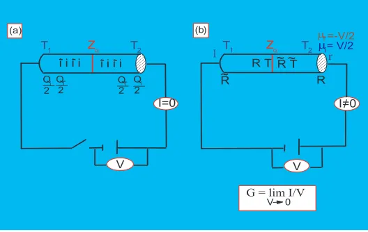
direct currentI through such a quantum wire can be computed simply by determining the difference between the static charge distributions at the right and left constriction of the wire, i.e. I =Qr−Ql. This is based on the assumption [19, 20], thatQ(t)∼(Qr−Ql)t∼
[image:7.612.164.428.174.341.2](ρr−ρl)t, where the ρs are the corresponding density distribution functions. Placing an
Figure 2: A conductance measurement. Part (a) represents the initial condition with no current flowing, i.e., I=0 and part (b),I 6= 0. The defect is placed in the middle of the wire and the left and right half are assumed to be at temperaturesT1 andT2, respectively.
impurity in the middle of the wire, we have to quantify the overall balance of particles of type i and anti-particles ¯ı carrying opposite charges qi = −q¯ı at the end of the wire
at different potentials. This information is of course encoded in the density distribution functionρr
i (θ, T, µi). In the described set up half of the particles of one type are already at
the same potential at one of the ends of the wire and the probability for them to reach the other is determined by the transmission and reflection amplitudes through the impurity. We assume that there is no effect coming from the constrictions of the wire, i.e. they are purely transmitting surfaces withT = ˜T = 1. One could, however, also consider a situation in which those constrictions act as boundaries, namely purely reflecting surfaces. The situation could be described with the same transport theory picture, see e.g. [19, 21, 22], but then the conductance can only be non-vanishing if the reflection amplitudes in the constrictions are non-diagonal in the particle degrees of freedom, such as for instance for sine-Gordon [23], that is in general affine Toda field theories with purely imaginary coupling constant or, in the massless limit, folded purely reflecting (transmitting) diagonal bulk theories.
According to the Landauer transport theory the direct current (DC) along the wire is given by
Iα~ = X
i
Ii~α(r, µli, µri) =X
i
qi
2
∞
Z
−∞
PrHEP unesp2002
= IB−
X
i
qi
2
∞
Z
−∞
dθhρri(θ, r, µri)|R~αi (θ)|2−ρir(θ, r, µli)|R˜iα~(θ)|2i , (2.2)
where we assume hereT1 =T2. The relation (2.2) is obtained from (2.1) simply by making
use of the fact that |R|2+|T|2= 1 (see section 2 in part I). Equation (2.2) has the virtue
that it extracts explicitly the bulk contribution to the current which we refer to as IB.
There are some obvious limits, namely a transparent and an impenetrable defect lim
|T~α|→1I
~
α =I
B and lim
|T~α|→0I
~
α= 0, (2.3)
respectively. A short comment is needed on the validity of (2.1). Apparently it suggests that when the parity between left and right scattering is broken, there is the possibility of a net current even when an external source is absent. In this picture we have of course not taken into account that charged particles moving through the defect will alter the potential, such that we did in fact not describe a perpetuum mobile. Thus the limitation of our analysis is that µl
i −µri has to be much larger than the change in the potential
induced by the moving particles.
Finally we want to compute the conductance from the DC current, which by definition is obtained from
G~α(r) =X
iG
~ α
i(r) =
X
i(µllim
i−µri)→0
Iiα~(r, µli, µri)/(µli−µri) (2.4)
and is of course a property of the material itself and a function of the temperature. In general the expressions in (2.1) tend to zero for vanishing chemical potential difference such that the limit in (2.4) is non-trivial.
Thus from the knowledge of the transmission matrix and the density distribution function we can compute the conductance.
2.1 The high temperature regime
Since the physical quantities require a solution of the TBA-equations, which up to now, due to their non-linear nature, can only be solved numerically, we have to resort in general to a numerical analysis to obtain the conductance for some concrete theories. However, there exist various approximations for different special situations, such as the high temperature regime. For large rapidities and small r, it is known [9] (here we only need the small modification of the introduction of a chemical potential µi) that the density of states can
be approximated by
ρi(θ, r, µi)∼
mi
4πe
|θ|∼ 1
2πrǫ(θ)
dεi(θ, r, µi)
dθ , (2.5)
where ǫ(θ) = Θ(θ)−Θ(−θ) is the step function, i.e. ǫ(θ) = 1 for θ > 0 and ǫ(θ) = −1 for θ < 0. In equation (1.17), we assume that in the large rapidity regime ρri(θ, r, µi) is
dominated by (2.5) and in the small rapidity regime by the Fermi distribution function. Therefore
ρri(θ, r, µi)∼
1 2πrǫ(θ)
d
PrHEP unesp2002
Using this expression in equation (2.1), we approximate the direct current in the ultraviolet by
lim
r→0I
~ α
i (r, µi)∼
qi 4πr ∞ Z −∞ dθln
1 + exp(−εi(θ, r, µli))
1 + exp(−εi(θ, r, µri))
d
ǫ(θ)|Ti~α(θ)|2
dθ , (2.7)
after a partial integration. For simplicity we also assumed here parity invariance, that is
|Tiα(θ)| = |T˜iα(θ)|. The derivation of the analogue to (2.7) for the situation when parity is broken is of course similar. Taking now the potentials at the end of the wire to be
µr
i =−µli =V /2, the conductance reads in this approximation
lim
r→0G
~ α
i(r)∼
qi 2πr ∞ Z −∞ dθ 1
1 + exp[εi(θ, r,0)]
dεi(θ, r, V /2)
dV V=0 d
ǫ(θ)|Ti~α(θ)|2
dθ . (2.8)
In order to evaluate these expressions further, we need to know explicitly the precise form of the transmission matrix, i.e. the concrete form of the defect. An interesting situation occurs when the defect is transparent or rapidity independent, that is |Ti~α(θ)| → |Ti~α|, in which case we can pursue the analysis further. Noting thatdǫ(θ)/dθ = 2δ(θ), we obtain
lim
r→0G
~ α
i(r)∼
qi
πr
|T~α i |2
1 + expεi(0, r,0)
dεi(0, r, V /2)
dV V=0 . (2.9)
The derivative dεi(0, r, V /2)/dV can be obtained by solving recursively
dεi(0, r, V /2)
dV =− r 2− X j Nij 1
1 + expεj(0, r, V /2)]
dεj(0, r, V /2)
dV , (2.10)
which results form a computation similar to a standard one in this context [9] leading to the so-called constant TBA-equations. Here only the asymptotic phases of the scattering matrix enter via Nij = limθ→∞[ln[Sij(−θ)/Sij(θ)]]/2πi. The values of εi(0, r,0) needed
in (2.9) can be obtained for small r in the usual way from the standard constant TBA-equations.
2.2 Free Fermion with defects
Let us exemplify the general formulae once more with the free Fermion. First of all we note that in this case in the TBA-equations (1.18) the kernelϕij is vanishing and the equation
is simply solved by
εi(θ, r, µi) =rmicoshθ−rµi. (2.11)
Therefore, we have explicit functions for the densities with (1.19) and (1.17)
ρi(θ, r, µi) =
1
2πmicoshθ and ρ
r
i (θ, r, µi) =
micoshθ/2π
1 + exp(rmicoshθ−rµi)
. (2.12)
According to (2.1) the direct current reads
Iα~(r, V) = qi 2
∞
Z
−∞
dθhρr¯ı (θ, r, V /2)|T¯ı~α(θ)|2−ρri(θ, r,−V /2)|Ti~α(θ)|2
PrHEP unesp2002
Using atomic units me=e=h=mi=qi= 1, we obtain explicitly with (2.12)
Iα~(r, V) = 1
π
∞
Z
0
dθ coshθsinh(rV /2)|T
~α(θ)|2
cosh(rcoshθ) + cosh(rV /2), (2.14)
for |T¯ıα(θ)| =|Tiα~(θ)|=|T˜ı¯α~(θ)|=|T˜iα(θ)|= |T~α(θ)|. Then by (2.4) the conductance results to
Gα~(r) =rme
2
h
∞
Z
0
dθ coshθ Tα~(θ)
2
1 + cosh(rmcoshθ) (2.15) in this case. We have re-introduced dimensional quantities instead of atomic units to be able to match with some standard results from the literature. The most characteristic features can actually be captured when we carry out the massless limit as indicated in section 2.3.2, which can be done even analytically. Substitutingt=eθ, we obtain
lim
m→0G
~
α(r)∼ e2
h
∞
Z
0
dt|T
~ α
L/R(t y/r)|2
1 + cosh(t) =
e2
h (
|T~α
L/R(t y/r)|2 for y≫r
|TL/R~α (y/r= 0)|2 for y≪r . (2.16)
We have identified here two distinct regions. When y ≪ r we can replace the left/right transmission amplitudes by their values aty/r = 0. When y≫ r the transmission ampli-tudes enter the expression as a strongly oscillatory function in which y/r plays the role of the frequency. It is then a good approximation to replace this function by its mean value as indicated by the overbar. It is straightforward to extend the expression (2.16) to the case when the assumption on Tα in (2.14) is relaxed and to the case with different values of y. To proceed further we need to specify the defect.
2.2.1 Transparent defects, |T~α|= 1
Let us first consider the easiest example, which supports the general working of the method. When the defect is transparent, i.e., |T~α| = 1, we can compute the expression for the conductance (2.15) directly in the large temperature limit and obtain the well known behaviour [24]
lim
r→0,|Tα~|→1G
~ α(r)
∼e
2
h(1− rm
2 ). (2.17) Alternatively, we obtain the expression (2.17) also from equation (2.9) and (2.11). In the massless limit of (2.16) we obtaine2/hwhich coincides with the result in [19]. However, we
should stress that we consider here purely massive cases and the massless limit only serves as a benchmark. Note that a transparent defect in this context does not necessarily mean the absence of the defect, since the transmission amplitude could be a non-trivial phase.
2.2.2 The energy operator defect Dα( ¯ψ, ψ) =gψψ¯
PrHEP unesp2002
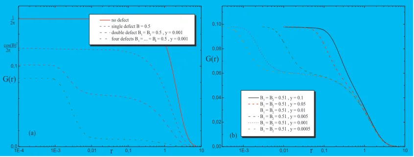
Figure 3: ConductanceG(r) for the complex free Fermion with the energy operator defects as a function of the inverse temperaturer, for fixed effective coupling constantB and (a) for varying amounts of defectsℓ= 0,1,2,4. (b) forℓ= 2 for varying distancesy.
temperature and increasing number of defects, the conductance decreases. Second we see several well extended plateaux. They can be reproduced with the analytical expressions obtained in the massless limit (2.16). To be able to compare with (2.15) we re-introduce atomic units for convenience, i.e. e2/h→1/2π. For a single defect there is only one plateau
and from (2.16) and the explicit expression forTα(θ) given in part I
Gα(r)∼ cos
2B
2π . (2.18)
For B = 0.5 the value 0.1226 is well reproduced in figure 3(a). The lower lying plateaux correspond to the region wheny≪r. In that case we obtain from (2.16) together with the expressions for the reflection and transmission amplitudes of the double and four defect systems derived in part I
Gα1α2(r) ∼ 1
2π
cos2B
1 + sin2B 2
for y ≪r, (2.19)
Gα1α2α3α4(r) ∼ 1
2π
cos4B
cos4B−2(1 + sin2B)2
2
for y ≪r. (2.20)
ForB = 0.5 the values 0.0624 and 0.0095 are well reproduced in figure 3(a) for ℓ= 2 and
ℓ= 4, respectively. The plateaux extending to the ultraviolet regime result from (2.16) and by taking mean values of the expressions for the reflection and transmission amplitudes of the double and four defect systems given in part I
Gα1α2(r) ∼ 2
π
1 + sin4B
(cos2(2B)−3)2 , for y≫r , (2.21)
Gα1α2α3α4(r) ∼ 1
4π +
cos8B
4π[cos4B−2(1 + sin2B)2]2, for y≫r. (2.22)
PrHEP unesp2002
reason for the increase from one to the next plateaux and why the curves are shifted precisely in the way as indicated in figure 3(b) when we change the distance between the defects. This phenomenon is attributed to resonances, namely the existence of very sharp picks in the probability of transmission for two or more defects (see figure 1 in part I).
If we now compare the expressions (2.18)-(2.22) with equations (3.34; part I)-(3.42; part I), we find complete agreement. This observation constitutes the central result of this work. We showed for a concrete integrable theory that the conductance computed by means of the newly formulated Kubo [1, 25] formula incorporating the presence of defects, and by means of Landauer [7] formula are in perfect agreement. More concrete examples of this agreement are provided in [1].
2.2.3 The SU(3)2 homogeneous sine-Gordon model, unstable particles
TheSU(3)2homogeneous sine-Gordon (HSG) model is the simplest of its kind and contains
only two self-conjugate solitons, which we denote by “+”, “−”, and one unstable particle, which we call ˜c. The corresponding scattering matrix was found [27] to be
S±±=−1, S±∓(θ) =±tanh
1 2
θ±σ− iπ
2
, (2.23)
which means the resonance pole associated to the formation ˜cis situated atθR=∓σ−iπ/2,
σ being a free parameter. Stable bound states may not be formed. Since only for S =±1 simultaneous reflection and transmission can occur [5], theSU(3)2-HSG model only admits
the presence of purely reflecting or transmitting defects. For the purely reflecting case, the expression (2.1) vanishes so that the only non-trivial situation we can consider is a transparent defect, i.e. |T|= 1. The results for the conductance after solving numerically the TBA equations (1.16) and (1.18) are depicted in figure 4. When solving (1.16) and (1.18) we have takenµR=−µL= 0.25.However, according to the definition (2.4) we should
really consider the limit (µR−µL)→0. The reason why we instead take µR−µL= 0.5 is
that for this model we can of course not solve the TBA-equations analytically, as for the free Fermion. On the contrary, the numerics become fairly involved and they do not allow for considering the extreme limit (µR−µL) → 0. However, we convinced ourselves that
the results depicted in figure 4 reproduce indeed the correct behaviour of the conductance, since computing G(r) in the deep ultraviolet limit for different values of µR−µL leads
always to the same plateau structure. We observe a relatively sharp increase in Gfor an energy scale 2 logr/2 ∼ −σ which corresponds to the onset of the unstable particle. In other words, only when a certain energy scale necessary for the excitation of the unstable particle is reached, the latter is formed and participates in the conducting process. All this information is encoded in the density ρri(θ, r, µi). Computing nowεi(θ,0,0) in a standard
TBA fashion we predict the plateaux from (2.9) analytically at 1/2π and 2(1 +√5)/(5 +
√
5)π. The last plateau corresponds to the deep ultraviolet limit, whereas the plateau at 1/2π coincides with the value (2.17) for a free Fermion theory when takinge/h= 1/2π.The reason is that the second plateau in figure 5 develops in the region when σ ≫ −2 logr/2, that is σ very large. In that limit we have limσ→∞S±∓(θ) = 1, such that the model
PrHEP unesp2002
[image:13.612.273.506.89.262.2]2.2.4 Resonances versus unstable
Figure 4: Conductance for theSU(3)2-HSG-model. particles
In the light of the results of subsec-tions 2.2.2 and 2.2.3 we can draw the conclusion that resonances in a dou-ble defect system and the presence of unstable particles may be described similarly [4]. Comparing figures 3(b) and 4, it is clear that the plateau struc-tures encountered do not differ much from each other. In particular, it seems that the parameteryin the double de-fect system and the resonance param-eterσin theSU(3)2-HSG model play
similar roles. Let us investigate more
precisely these similarities, which from an intuitive point of view appear rather natural. In the context of theories possessing unstable particle in their spectra, a very clear picture which explains the relatively sharp onset of the conductance with increasing tem-perature can be provided. The temtem-perature at which this onset occurs, say TC can be
related directly to the energy scale at which the unstable particle is formed, since then it starts to participate in the conducting process. The Breit-Wigner formula [26] provides in this case the expressions for the massMc˜and the decay width Γ˜c of the unstable particle
˜
c. Supposing that the particle ˜c is formed in the scattering process between particles of typesiandj of massesmi, mj,this is reflected by a pole in Sij(θ) atθR=σ−iσ¯. Setting
¯
σ =π/2, as corresponds to the model at hand, the Breit-Wigner formula for large values of the resonance parameter σ gives
M˜c≈
1
√
2
√m
imjexp|σ|/2 and Γ˜c ≈
p
2mimjexp|σ|/2. (2.24)
Since a renormalization group flow is provided by mappingM → r M, one observes that the quantity M˜c(r, σ) = rM = reσ/2 should remain invariant under the renormalization
group flow. That means that if r1 is the onset energy for the unstable particle ˜cforσ=σ1
and r2 is the onset energy for σ =σ2, the conductance must satisfy the following scaling
law
G(r1, σ1) =G(r2, σ2) for r1eσ1/2 =r2eσ2/2. (2.25)
This means we can control the position of the onset in the conductance byMc˜(r, σ).
Analyzing now the scaling behaviour of the conductance for the double defect system studied in subsection 2.2.2 we find
G(r1, y1) =G(r2, y2) for
r1
y1
= r2
y2
, (2.26)
PrHEP unesp2002
that the net result with regard to the conductance is the same, the origin of the onset is different. Whereas for the HSG-model it resulted from a change in the density distribution function ρri(θ, r, µi) it is now triggered by the structure of |Tα(θ)|. Since for the free
Fermion the function ρri keeps its overall shape and just translates as the temperature is changed, the onset of the conductance occurs when the maxima of |Tα(θ)| are reached. By analyzing the concrete expression of Tα(θ) for the energy operator defect (see part I)
it is easy to verify that for a double defect
Tα1α2(θ= ln
(2n+ 1)π y
)≈1 for n∈Z. (2.27)
Drawing an analogy to the scattering matrix of the HSG-model the values of θ for which
Tα1α2(θ) is maximal play the same role as the value θ
R = σ −iπ/2 corresponding to
the resonance pole of the S-matrix. In that sense we can make the identification σn =
ln [(2n+ 1)π/y]. There are however some differences between both systems, since in the case of the SU(3)2-HSG model the onset of the conductance is due to a single unstable
particle, whereas for the double defect system the same effect can be attributed to several maxima of the transmission probability. The other important difference is thaty is now a measurable quantity, so that the “mass” of the resonances can be experimentally accessible.
2.2.5 Multiple plateaux
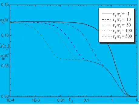
[image:14.612.275.504.419.593.2]Up to now, we have observed that we always obtain essentially two plateaux in the con-ductance, no matter how many (≥2) and what type of defects we implement. The natural question arising at this point is whether
Figure 5: Conductance G(r2) for the complex free Fermion with the energy operator defects as a function of the inverse temperature r2, for fixed effective cou-pling constantB = 0.5 and varying temperature ratios in the two halves of the wire.
it is possible to have a set up which leads to a more involved plateaux struc-ture. It is clear that if we had many defects in a row separated far enough from each other such that the relax-ation time of the passing particles is so large that they could be treated as single rather than multiple defects, then any desired type of multiple plateau structure could be obtained. In this case the conductance is simply the sum of the expressions one has for each de-fect independently. Recalling the ori-gin of the different plateaux, there is another slightly less obvious option. The density distribution function ρr
is a peaked function of the rapidity
PrHEP unesp2002
the rapidity variable or change their amplitudes, respectively (see section 2, part I). There-fore the last option left is to change theρrs, which is possible by varying the temperature. Choosing now a configuration as in figure 2 with different temperatures T1 and T2, one
can “create” a second plateau at half the height of the original one. The reason for this is simply that the cooled half of the wire will cease to contribute to the conductance as can be directly deduced from (2.15). We depict the results of our computations in figure 5. From this it also obvious that if we only cool the fraction x of the wire, the lowest plateau will be positioned at the height x times the height of the upper plateau. Thus, by combining these different configurations, i.e., different temperatures or defects, we could produce any desired plateau structure.
3. Conclusions and open problems
In this section I will present the main conclusions of my talk and also of part I, since the main aim of this work was actually to compare the two theoretical descriptions presented in the two parts. In our work we have exploited the special features of 1+1 dimensional integrable quantum field theories in order to compute the DC conductance in an impurity system. For this purpose several non-perturbative techniques have been used. As the main tools we employed the thermodynamic Bethe ansatz in a Landauer transport theory computation and the form factor expansion in the Kubo formula.
The comparison between the Kubo formula (1.1; part I) and the Landauer formula (2.1) yields in particular an identical plateau structure for the DC conductance in the ultraviolet limit.
We have explained to what extend integrability can be exploited in order to determine the reflection and transmission amplitudes through a defect. Unfortunately, for the most interesting situation in this context, namely whenR/R˜ and T /T˜ are simultaneously non-vanishing, the Yang-Baxter bootstrap equations narrow down the possible bulk theories to those which possess rapidity independent scattering matrices [16, 5]. By means of a relativistic potential scattering theory we computed for several types of defects the R/R˜s andT /T˜s, thus enlarging the set of examples available at present. We confirm that for real potentials parity is preserved, but otherwise essentially all possible combinations of parity breaking can occur. From the knowledge of the single defect amplitudes the multiple defect amplitudes, which exhibit the most interesting physical behaviours, can be computed in a standard fashion [28, 29].
We have newly proposed a Kubo formula [25] which accommodates the situation when defects are present (1.1; part I). We evaluated the current-current correlation functions occurring in there by means of a non-perturbative method based on integrability, namely the bootstrap form factor approach [30, 31]. We provide closed formulae which solve explicitly the defect recursive equations involving any arbitrary number of particles. We predict the plateaux in the conductance as a function of the temperature analytically.
PrHEP unesp2002
when considered per unit length. By means of the TBA we compute the density distribu-tion funcdistribu-tions and use them to evaluate the Landauer conductance formula (2.1) for various defects in a complex free Fermionic theory. Also in this case, we predict analytically the most prominent features in the conductance as a function of the temperature, i.e. the plateaux.
There exist various investigations, e.g., [32, 19, 21, 33] for conformal (massless) theories with defects, which exploit the original folding idea of Wong and Affleck [32]. The idea is that a conformal field theory with a purely transmitting or reflecting defect can be mapped into a boundary theory, i.e. a theory living in half space, which has the advantage that the full restriction of modular invariance can be exploited in the construction of boundary states as pioneered by Cardy [34]. Apparently the folding procedure could lead to non-trivial solutions for the reflection and transmission amplitudes starting with a purely reflecting or transmitting theory. However, one should stress that the folding is carried out on the basis of the field content of the conformal field theory, whereas our analysis is based on a particle description, namely we take the ZF-algebra as our starting point. Therefore, the transmission and reflection amplitudes obtained by means of the folding technique can not be compared with the objects we study here, even in the conformal limit.
In this context, there are several interesting open issues. Most challenging is to treat in full generality the massive and temperature dependent case of (1.1; part I). Unfortunately, the formulation of non-perturbative methods does not yet cover that situation [6] and it remains to be clarified how the form factor bootstrap program for the computation of two-point functions can be extended to that case. It would be further interesting to compute thermodynamic quantities per unit length by means of the TBA and to develop methods for the systematic classification of integrable defects.
Proceeding further in our investigation of the applications of integrable models to the description of realistic physical systems, we have established thatcoupling an impurity in a quantum wire to an external monochromatic electromagnetic field leads to high harmonic generation [2]. Harmonic generation i.e., the emission of multiples of the incoming fre-quency when a system is coupled to a monochromatic field, has been widely studied in the context of atomic physics. However, up to now there were no results for solid state materials. The concrete system we have studied is a quantum wire described by means of the Dirac equation doped with a defect which couples minimally to an external field of frequencyω. Considering separately the situations corresponding to a single and a double defect system we observed that, for the particular type of defect treated, only even multi-ples of the incoming frequency are emitted for the single defect, whereas all even and odd multiples are generated for the double defect system. These features are observed both in the Fourier expansion of the transmission probability through the defect and in the emis-sion spectrum of the dipole momentum. It would be extremely interesting to confirm our findings experimentally.
Acknowledgments
PrHEP unesp2002
talks, for financial support and for making the celebration of the 50th anniversary of the
Instituto de F´ısica Te´orica (IFT) a very enjoyable and rewarding event. In addition, we would like to thank Carla Figueira de Morisson Faria (Max Born Institut Berlin) and Frank G¨ohmann (Universit¨at Bayreuth) for their participation in [2] and [5], respectively. We are also grateful to the Deutsche Forschungsgemeinschaft (Sfb288) for financial support.
References
[1] O.A. Castro-Alvaredo and A. Fring, From integrability to conductance, impurity systems, hep-th/0205076.
[2] O.A. Castro-Alvaredo, A. Fring and C. Figueira de Morisson Faria, Relativistic treatment of harmonics from impurity systems in quantum wires, cond-mat/0208128.
[3] O.A. Castro-Alvaredo and A. Fring, Nucl. Phys.B618[FS] (2001) 437.
[4] O.A. Castro-Alvaredo and A. Fring, Unstable particles versus resonances in impurity systems, conductance in quantum wires,cond-mat/0112199.
[5] O.A. Castro-Alvaredo, A. Fring and F. G¨ohmann,On the absence of simultaneous reflection and transmission in integrable impurity systems, hep-th/0201142.
[6] O.A. Castro-Alvaredo and A. Fring, Nucl. Phys.B636(2002) 611.
[7] R. Landauer,IBM J. Res. Dev. 1(1957) 223;Philos. Mag. 21 (1970) 863 ; M. B¨uttinger,
Phys. Rev. Lett.57 (1986) 1761.
[8] C.N. Yang and C.P. Yang,Phys. Rev.147(1966) 303;J. Math. Phys.10(1969) 1115.
[9] Al.B. Zamolodchikov,Nucl. Phys.B342(1990) 695.
[10] M.J. Martins,Nucl. Phys. B426 [FS] (1994) 661.
[11] A. LeClair, G. Mussardo, H. Saleur and S. Skorik,Nucl. Phys.B453(1995) 581.
[12] A.B. Zamolodchikov and Al.B. Zamolodchikov, Ann. of Phys. 120(1979) 253; L.D. Faddeev, Sov. Sci. Rev. Math. Phys.C1(1980) 107.
[13] I.V. Cherednik, Theor. Math. Phys.61(1984) 977.
[14] E.K. Sklyanin, J. Math. Phys.A21(1988) 2375.
[15] A. Fring and R. K¨oberle,Nucl. Phys. B421(1994) 159;Nucl. Phys. B419 [FS](1994) 647;
Int. J. of Mod. Phys. A10(1995) 739.
[16] G. Delfino, G. Mussardo and P. Simonetti,Phys. Lett.B328(1994) 123,Nucl. Phys. B432
(1994) 518.
[17] O.A. Castro-Alvaredo, A. Fring, C. Korff and J.L. Miramontes,Nucl. Phys.B575(2000) 535.
[18] T.R. Klassen and E. Melzer,Nucl. Phys.B338(1990) 485;Nucl. Phys. B350(1991) 635;
Nucl. Phys. B370(1992) 511.
[19] P. Fendley, A.W.W. Ludwig and H. Saleur,Phys. Rev.B52(1995) 8934.
[20] F. Lesage, H. Saleur and S. Skorik,Nucl. Phys. B474 (1996) 602.
[21] P. Fendley, A.W.W. Ludwig and H. Saleur,Phys. Rev. Lett.74 (1995) 3005.
PrHEP unesp2002
[23] S. Ghoshal and A.B. Zamolodchikov,Int. J. of Mod. Phys. A9(1994) 3841.
[24] C.L. Kane and M.P.A. Fisher,Phys. Rev.B46 (1992) 15233.
[25] R. Kubo,Can. J. Phys. 34 (1956) 1274.
[26] G. Breit and E.P. Wigner,Phys. Rev.49519 (1936).
[27] J.L. Miramontes and C.F. Fern´andez-Pousa,Phys. Lett.B472(2000) 392.
[28] C. Cohen-Tannoudji,Quantum Mechanic, (John Wiley & Sons, New York, 1977).
[29] E. Merzbacher,Quantum Mechanic, (John Wiley & Sons, New York, 1970).
[30] P. Weisz,Phys. Lett. B67 (1977) 179; M. Karowski and P. Weisz,Nucl. Phys. B139(1978) 445.
[31] F.A. Smirnov,Form Factors in Completely Integrable Models of Quantum Field Theory,
Advanced Series in Mathematical Physics, Vol. 14, World Scientific, Singapore, 1992.
[32] E. Wong and I. Affleck,Nucl. Phys. B417 (1994) 403.
[33] M. Oshikawa and I. Affleck,Nucl. Phys. B495 (1997) 533; A. LeClair, A.W.W. Ludwig and G. Mussardo,Nucl. Phys. B512 (1998) 523; A. LeClair and A.W.W. Ludwig,Nucl. Phys.
B549 (1999) 546; C. Nayak, M.P.A. Fisher, A.W.W. Ludwig and H.H. Lin,Phys. Rev.B59
(1999) 15694; T. Quella and V. Schomerus,Symmetry breaking boundary states and defect lines, hep-th/0203161.