City, University of London Institutional Repository
Citation
:
Castro-Alvaredo, O. & Fring, A. (2002). From integrability to conductance, impurity systems. Nuclear Physics B, 649(3), pp. 449-490. doi:10.1016/S0550-3213(02)01029-5
This is the accepted version of the paper.
This version of the publication may differ from the final published
version.
Permanent repository link: http://openaccess.city.ac.uk/16431/
Link to published version
:
http://dx.doi.org/10.1016/S0550-3213(02)01029-5Copyright and reuse:
City Research Online aims to make research
outputs of City, University of London available to a wider audience.
Copyright and Moral Rights remain with the author(s) and/or copyright
holders. URLs from City Research Online may be freely distributed and
linked to.
City Research Online: http://openaccess.city.ac.uk/ [email protected]
arXiv:hep-th/0205076v1 8 May 2002
Berlin Sfb288 Preprint hep-th/0205076
From integrability to conductance, impurity systems
Olalla Castro-Alvaredo and Andreas Fring
Institut f¨ur Theoretische Physik, Freie Universit¨at Berlin, Arnimallee 14, D-14195 Berlin, Germany
Abstract
We compute the DC conductance with two different methods, which both exploit the integrability of the theories under consideration. On one hand we determine the conductance through a defect by means of the thermodynamic Bethe ansatz and standard relativistic potential scattering theory based on a Landauer transport theory picture. On the other hand we propose a Kubo formula for a defect system and evaluate the current-current two-point correlation function it involves with the help of a form factor expansion. For a variety of defects in a fermionic system we find excellent agreement between the two different theoretical descriptions.
PACS numbers: 73.50.Bk, 73.40.-c, 72.10.-d, 11.10Kk, 05.30.-d
Contents
1 Introduction 2
2 Determining the defect scattering matrices 3
2.1 Defect Yang-Baxter equations . . . 3
2.2 Multiple defects . . . 5
2.3 Free Fermion with defects . . . 7
2.3.1 Transmission and reflection amplitudes . . . 8
2.3.2 The energy operator defect Dα(¯ψ, ψ) =gψψ¯ . . . 9
2.3.3 Transparent defects, D0(¯ψ, ψ) = 0,Dβ(¯ψ, ψ) =gψγ¯ 1ψ . . . 12
2.3.4 Energy insensitive defects,Dγ(¯ψ, ψ) =gψγ¯ 5ψ,Dδ±(¯ψ, ψ) =gψ¯(γ1±γ5)ψ 12 2.3.5 Luttinger liquid type Dε(¯ψ, ψ) = ¯ψ(g 1+g2γ0)ψ . . . 13
2.3.6 The defects Dη±(¯ψ, ψ) =gψ¯(1±γ5)/2ψ . . . 14
2.3.7 The defects Dλ±(¯ψ, ψ) =gψ¯(γ0±γ1)/2ψ . . . 14
3 Conductance from the Landauer formula 15 3.1 Conductance through an impurity . . . 15
3.2 Defect TBA equations . . . 16
3.3 Thermodynamic quantities . . . 19
3.4 The high temperature regime . . . 19
3.5 Free Fermion with defects . . . 20
3.5.1 Energy insensitive defects,D0(¯ψ, ψ) = 0, Dβ(¯ψ, ψ), Dγ(¯ψ, ψ),Dδ±(¯ψ, ψ) 21 3.5.2 The energy operator defect Dα(¯ψ, ψ) =gψψ¯ . . . 21
3.5.3 Resonances versus unstable particles . . . 23
3.5.4 Multiple plateaux . . . 23
4 Conductance from the Kubo formula 24 4.1 Conductance through an impurity . . . 25
4.2 Realization of the defect operator . . . 28
4.3 Defect matrix elements . . . 29
4.4 Free Fermion with defects . . . 30
4.4.1 Defect matrix elements . . . 30
4.4.2 Conductance in theT =m= 0 regime . . . 32
4.4.3 Energy insensitive defects,D0(¯ψ, ψ) = 0, Dβ(¯ψ, ψ),Dγ(¯ψ, ψ),Dδ±(¯ψ, ψ) 34 4.4.4 The energy operator defect D(¯ψ, ψ) =gψψ¯ . . . 35
1
Introduction
Conductance (conductivity) measurements belong to the easiest and most direct experiments which can be carried out. They attract a lot of attention, due to the fact that in general they can be performed without perturbing very much the behaviour of the system, e.g. a rigid-lattice bulk metal, such that the uncertainty of experimental artefacts is reduced to a minimum. There exist various well-known theoretical descriptions, such as semi-classical transport theories (Landauer [1] and Boltzmann-Drude [2]), dynamical linear-response theory [3, 4] and also Green function linear-response theory [5]. To carry out the latter, in particular at finite temperature, is still poorly understood in generality [6], even in 1+1 space-time dimensions [7]. Since recent experimental progress allows conductance measurements also in 1+1 space-time dimensions [8], one can on the theoretical side fully exploit the special features of low dimensionality.
It is in particular very suggestive to exploit the full scope of non-perturbative techniques which have been developed in the context of integrable quantum field theories in 1+1 space-time dimensions, such as the thermodynamic Bethe ansatz (TBA) [9, 10] and the form factor bootstrap approach [11, 12]. Generalizing the Landauer transport picture a proposal for the conductance through a quantum wire with a defect (impurity) has been made in [13, 14]
Gα
(T) =X i
lim (µl
i−µri)→0 qi
2
∞
Z
−∞
dθhρri(θ, T, µli)|Tα
i (θ)|2−ρir(θ, T, µri)|T˜ α i (θ)|2
i
, (1.1)
which we only modify to accommodate parity breaking, known to occur in integrable lattice models, see e.g. [15]. This means in particular we allow the transmission amplitudes to be different for a particle of typeiwith chargeqipassing with rapidityθthrough a defect of type α from the left Tα
i (θ) and right ˜T α
i (θ). The density distribution function ρri(θ, T, µi), being a function the temperature T, and the potential at the left µli and rightµri constriction of the wire, can be determined by means of the TBA. We have already restricted (1.1) to the abelian (diagonal) situation. It is clear that the effect resulting from the defect is most interesting when |Tα
i (θ)| 6= 1, which requires the occurrence of simultaneous transmission and reflection (see (2.6), (2.17)). In this paper we will therefore be mainly interested in that situation. One may adapt (1.1) also to the case of pure reflection, which physically describes the influence of the constriction to the conducting process. From the previous statement it is clear that such boundary theories are only interesting in this physical context when they are non-abelian.
The other prominent way of determining the conductance is a result from linear response theory, which yields an expression for the conductance in form of the Fourier transform of the current-current two-point correlation function. This Kubo formula has been adopted to the situation with a boundary [16]. As we mentioned, this will only capture effects coming from the constriction of the wire, we propose here a generalization to the analogous situation as described in (1.1), i.e. when a defect is present
Gα
(T) =−lim ω→0
1 2ωπ2
∞
Z
−∞
dt eiωt hJ(t)ZαJ(0)iT,m. (1.2)
Here the defect operatorZαenters in-between the two currentsJ within the temperature and
The main purpose of this manuscript is to compare the two alternative descriptions (1.1) and (1.2) for massive bulk theories with a defect which allows for simultaneous reflection and transmission. There exist various investigations, e.g., [17, 13, 14, 18] for conformal (massless) theories with defect, which exploit the original folding idea of Wong and Affleck [17]. The idea is that a conformal field theory with a purely transmitting or reflecting defect can be mapped into a boundary theory, i.e. a theory living in half space, which has the advantage that the full restriction of modular invariance can be exploited in the construction of boundary states as pioneered by Cardy [19]. Since this folding idea relies on the vanishing of either the reflection or transmission, our considerations do in general not reduce to that set up, even in the conformal limit. As was already pointed out in [17], and as can be seen directly from (1.1) and (1.2), in that case the conductance is less interesting because it is either zero or perfect for abelian theories.
In section 2 we outline the procedure of how the defect scattering matrices may be deter-mined, since they are needed as input in both approaches. In section 3 we newly formulate the defect TBA equations and use them to determine the density distribution functions. We evaluate numerically the Landauer formula (1.1) for various defects and provide some analyt-ical approximations in certain regimes. In section 4 we propose a Kubo formula (1.2) for a configuration in which an impurity is present and compute the current-current two-point cor-relation functions occurring in there by means of a form factor expansion. We find very good agreement between (1.1) and (1.2) for the complex free Fermion theory with various types of defects. Our final conclusions and an outlook into open problems is provided in section 5.
2
Determining the defect scattering matrices
An essential input required in both non-perturbative methods which are exploited to compute the conductance (1.1) and (1.2), that is the TBA and the form factor bootstrap approach, respectively, is the knowledge of the exact (defect) scattering matrix. It is one of the most intriguing facts of two dimensional quantum field theories that these matrices can be deter-mined exactly to all orders in perturbation theory. In the following section we will recall how much (little) of this approach can be carried over to the situation when defects are present and compute explicitly the transmission and reflection amplitudes for a variety of concrete defects.
2.1 Defect Yang-Baxter equations
A cornerstone in the context of integrable models in 1+1 space-time dimensions are the Yang-Baxter equations [20]. They can be derived most easily simply by exploiting the associativity of the so-called Zamolodchikov-Faddeev (ZF) algebra [21] and its extended version which includes an additional generator representing a boundary [22, 23, 24] or a defect [25, 26]. Indicating particle types by Latin and degrees of freedom of the impurity by Greek letters, the “braiding” (exchange) relations of annihilation operators Zi(θ) of a particle of type i moving with rapidity θand defect operators Zα in the stateα can be written as
Zi(θ1)Zj(θ2) = Sijkl(θ1−θ2)Zk(θ2)Zl(θ1), (2.1)
Zi(θ)Zα = Rjβiα(θ)Zj(−θ)Zβ +Tiαjβ(θ)ZβZj(θ), (2.3)
ZαZi(θ) = R˜jβiα(−θ)ZβZj(−θ) + ˜Tiαjβ(−θ)Zj(θ)Zβ. (2.4)
The bulk scattering matrix is indicated by S, and the left/right reflection and transmission amplitudes through the defect are denoted by R/R˜ and T /T˜, respectively. We employed Einstein’s sum convention, that is we assume sums over doubly occurring indices. We suppress the explicit mentioning of the dependence of Zα on the position in space and assume for the time being that it is included in α. For the treatment of a single defect this is not relevant, but it will become important when we consider multiple defects. The same relations hold when we replace the annihilation operators by the creation operators Zi†(θ) with R/R˜,T /T˜
and S replaced by their complex conjugates. The algebra (2.3)-(2.4) can be used to derive various relations amongst the scattering amplitudes. Using extended ZF-algebra twice leads to the constraints
Sijkl(θ)Sklmn(−θ) = δmi δnj, (2.5)
Rjβiα(θ)Rjβkγ(−θ) +Tiαjβ(θ) ˜Tjβkγ(−θ) = δkiδγα, (2.6)
Riαjβ(θ)Tjβkγ(−θ) +Tiαjβ(θ) ˜Rkγjβ(−θ) = 0. (2.7)
The same equations also hold after performing a parity transformation, that is for R ↔ R˜
and T ↔T˜ in (2.6)-(2.7). From the associativity of the extended ZF-algebra one derives the equations [22, 23, 24, 25, 26]
S(θ12)[I⊗Rβα(θ1)]S(ˆθ12)[I⊗Rβγ(θ2)] = [I⊗Rαβ(θ2)]S(ˆθ12)[I⊗Rβγ(θ1)]S(θ12), (2.8)
S(θ12)[I⊗Rβα(θ1)]S(ˆθ12)[I⊗Tβγ(θ2)] =Rγβ(θ1)⊗Tαβ(θ2), (2.9)
S(θ12)[Tαβ(θ2)⊗Tβγ(θ1)] = [Tαβ(θ1)⊗Tβγ(θ2)]S(θ12), (2.10)
where we employed the convention (A⊗B)klij =AkiBjl for the tensor product and abbreviated the rapidity sum ˆθ12=θ1+θ2 and differenceθ12 =θ1−θ2. Once again the same equations also hold for R↔ R˜ and T ↔T˜. Starting with another initial asymptotic state one derives [26]
Rαβ(θ1)⊗R˜γβ(θ2) = Rγβ(θ1)⊗R˜αβ(θ2), (2.11)
[Tαβ(θ2)⊗I]S(ˆθ12)[ ˜Rγβ(θ1)⊗I]S(θ12) = Tβγ(θ2)⊗R˜αβ(θ1), (2.12) [I⊗T˜αβ(θ2)]S(ˆθ12)[I⊗Rγβ(θ1)]S(θ12) = Rβα(θ1)⊗T˜βγ(θ2), (2.13) [Tαβ(θ1)⊗I]S(ˆθ12)[ ˜Tβγ(θ2)⊗I] = [I⊗T˜αβ(θ2)]S(ˆθ12)[I⊗Tβγ(θ1)]. (2.14) On the basis of the equations (2.8)-(2.10), it was shown in [25], for the abelian case without defect degrees of freedom, that one can not have reflection and transmission simultaneously. In [26] this result was extended to the non-abelian parity breaking case and it was proven that for the simultaneous occurrence of reflection and transmission the scattering matrix has to be rapidity independent and of the form
with P being a permutation operator and σ a constant matrix. When assuming in addition that σ is a diagonal matrix with the propertyσijσji = 1, the free Fermion (σij =σji=−1), free Boson (σij = σji = 1) and also the Federbush model [27] and the generalized coupled Federbush models [28] are solutions to (2.15).
As a further set of consistency equations, which serve for the determination of the defect scattering matrix, we report the crossing relations, which are as usual less obvious to justify. In analogy to the relations which have to hold for the bulk scattering matrixSij(θ) =Si¯(iπ−θ) =
Sji∗(−θ), (¯ is the anti-particle of j and ∗ denotes the complex conjugation) we deduce from (2.3)-(2.4) the crossing-hermiticity relations
Rα¯(θ) = R˜α¯(−θ)∗ =Sj¯(2θ) ˜Rαj(iπ−θ), (2.16)
T¯α(θ) = T˜¯α(−θ)∗= ˜Tjα(iπ−θ). (2.17)
The first equalities follow when taking Zi†(θ)∗ =Zi(θ) and Zα =Zα†. The latter relations in (2.17) simply result by considering the relations forS while letting one of the particles freeze, i.e., setting its rapidity to zero, and viewing it as a defect. Relations (2.16) are obtainable in a similar fashion as the interpretation put forward in [29, 24]. Our equations (2.16) and (2.17) disagree slightly from the crossing relations in [29, 24, 25, 30], which is due to the fact that when parity is broken real analyticity is replaced by Hermitian analyticity [31]. Later on in our example, this will also be reflected in the representation of the free Fermion field (2.35), being Dirac rather than Majorana. There is of course no consequence of this choice of conventions on the physics, since the ambiguity just exploits the fact that only the moduli of these amplitudes are observable.
Similar as for the bulk scattering matrices an additional powerful constraint results from the singularity structure of the defect scattering amplitudes. In [26] it was shown that the defect does not admit any excited state once one demands a simultaneous occurrence of reflection and transmission. Supposing that the defect scattering matrices have a pole on the imaginary axis atiθ0 ∈iR, the corresponding residues are therefore constraint as
Res θ→iθ0R
α
j(θ) = Res θ→iθ0
˜
Rαj(θ) = Res θ→iθ0T
α
j (θ) = Res θ→iθ0
˜
Tjα(θ)
<0 for θ0 ∈(0, π)
>0 for θ0 ∈/(0, π) . (2.18)
The intervals (0, π) are understood to be mod 2π. Hence, there is no pole with positive residue in the physical sheet.
2.2 Multiple defects
we shall therefore focus on the diagonal case from now onwards. We compute
Zi(θ)ZαZβ = Rαβi (θ)Zi(−θ)ZαZβ+Tiαβ(θ)ZαZβZi(θ), (2.19)
ZαZβZi(θ) = R˜αβi (−θ)ZαZβZi(−θ) + ˜Tiαβ(−θ)Zi(θ)ZαZβ, (2.20)
where we have now introduced overall transmission and reflection amplitudes corresponding to two defects
Tiαβ(θ) = T α
i (θ)Tiβ(θ) 1−Rβi(θ) ˜Rα
i(θ)
, Rαβi (θ) =Rαi(θ) +R β
i(θ)Tiα(θ) ˜Tiα(θ) 1−Rβi(θ) ˜Rα
i(θ)
, (2.21)
˜
Tiαβ(θ) = T˜ α
i (θ) ˜Tiβ(θ) 1−Rβi(θ) ˜Rα
i(θ)
, R˜αβi (θ) = ˜Rβi(θ) +R α
i(θ)Tiβ(θ) ˜Tiβ(θ) 1−Rβi(θ) ˜Rα
i(θ)
. (2.22)
The term [1 −Rβi(θ) ˜Rα
i(θ)]−1 =
P∞
n=1(R
β
i(θ) ˜Rαi(θ))n results from the infinite number of reflections which we have in-between the two defects, well known from Fabry-Perot type devices of classical and quantum optics. For the case T = ˜T , R = ˜R the expressions (2.21) and (2.22) coincide with the formulae proposed in [32]. When absorbing the space dependent phase factor into the defect matrices, the explicit example presented in [25] for the free fermion perturbed with the energy operator agree almost forT = ˜T , R = ˜R with the general formulae (2.21). They disagree in the sense that the equality of Rαβi (θ) and ˜Rαβi (θ) does not hold for generic α, β as stated in [25].
It is now straightforward to extend the expressions to an arbitrary number of defects, say
n, in a recursive manner
Tα i (θ) =
Tα1...αk
i (θ)T
αk+1...αn
i (θ) 1−R˜α1...αk
i (θ)R
αk+1...αn
i (θ)
, 1< k < n , (2.23)
Rα
i (θ) = Rα1...αi k(θ) +
Rαk+1...αn
i (θ)Tiα1...αk(θ) ˜Tiα1...αk(θ) 1−R˜α1...αk
i (θ)R
αk+1...αn
i (θ)
, 1< k < n . (2.24)
For convenience we encoded here the defect degrees of freedom into the vectorα={α1,· · ·, αn}.
Similar expressions also hold for ˜Tα
i (θ) = ˜Tiα1...αn(θ) and ˜R α
i (θ) = ˜Riα1...αn(θ). It is clear that from the knowledge of the single defect amplitudes we are now in the position to compute the corresponding quantities for multiple defects just by nesting successively the expressions (2.23) and (2.24) for increasing values of ninto each other. Nonetheless, in general one does not succeed to provide simple analytical expressions for n-defect amplitudes and a different description is useful.
Alternatively, we can define, in analogy to standard quantum mechanical methods (see e.g. [33, 34]), a transmission matrix which takes the particle from one side of the defect to the other. From the braiding relations (2.3) and (2.4), we obtain with the help of the unitarity relations (2.6) and (2.7)
Zα1. . . ZαnZi(θ) Zα1. . . ZαnZi(−θ)
=
n Y k=1
Miαk(θ)
!
Zi(θ)Zα1. . . Zαn Zi(−θ)Zα1. . . Zαn
, (2.25)
with
Miαk(θ) =
Tαk
i (θ)−1 −R αk
i (θ)T αk
i (θ)−1
−Rαk
i (−θ)Tiαk(−θ)−1 Tiαk(−θ)−1
This means alternatively to the recursive way (2.23) and (2.24), we can also compute the multi-defect transmission and reflection amplitudes as
Tα i (θ) =
n Y k=1
Miαk(θ)
!−1
11
, Rα
i (θ) =− n Y k=1
Miαk(θ)
!
12
n Y k=1
Miαk(θ)
!−1
11
. (2.27)
One may convince oneself that this formulation is indeed the same as (2.23) and (2.24). It has, however, the virtue that it allows for a more elegant computation of the band structures. In particular, it is most suitable for numerical computations, since it just involves matrix multiplications rather than recurrence operations.
Let us now consider the case in which all the defects are of the same typeα, equidistantly separated by an amountyand sendn→ ∞. First of all we have to include now explicitly the dependence of the defect on its position into the discussion. We assume
n Y l=1
Miα(x=ly) = n Y l=1
QyMiα(x= 0) l
Q−ny1, Qy =
eiky 0 0 e−iky
, (2.28)
wherekcorresponds to the wavevector of the lattice. Taking thenn→ ∞this accommodates Bloch’s theorem (e.g., [33]) for the relativistic set-up. The simple requirement, that the product of transmission matrices limn→∞Qnl=1Miα(x =ly) remains finite, leads now in the usual way to a restriction for the allowed energies, that is to band structures. To see when this is the case we can exploit the r.h.s. of the first equation in (2.28) and diagonalize the matrix QyMiα(x = 0). Then it is clear that the limit n→ ∞ only remains finite when the eigenvalues of this matrix are not real
λi,α∈/R. (2.29)
The eigenvalues are computed to
λi,α1,2 = χαi(θ)± q
χαi(θ)2−T˜α
i (−θ)/Tiα(−θ), (2.30)
χαi(θ) = [e ikyTα
i (θ)−1+e−iky( ˜Tiα(θ)∗)−1]
2 . (2.31)
In the parity invariant case the criterium (2.29) becomes simpler. From (2.30) and (2.31) follows in that case that the allowed energies in the infinite lattice have to respect
χαi(θ) = Re[eikyTiα(θ)−1]<1, forT = ˜T . (2.32)
In other words particles are only allowed to travel in the system with rapidities for which the inequality (2.32) holds. In conclusion, this means the determination of the transmission amplitudes for a single defect is sufficient to determine multiple defects and the energy band structure. Let us illustrate the working of this general formulae with a concrete example.
2.3 Free Fermion with defects
different point of view. In [35, 29, 25] the defect line has the form of the energy operator and in [30] also a perturbation in form of a single Fermion has been considered. In this manuscript we want to enlarge the class of perturbations having in mind to obtain various different kinds of structural and physical behaviours.
Let us consider the Lagrangian density for a complex free Fermionψ withℓdefects∗
L= ¯ψ(iγµ∂µ−m)ψ + ℓ−1 X n=0
δ(x−xn)Dαn(¯ψ, ψ), (2.33)
where we describe the defect by the functions Dαn(¯ψ, ψ), which we assume to be linear in
the Fermi fields ¯ψ and ψ. In the following we will restrict ourselves mainly to the case of equidistantly distributed defects of the same type, i.e. xn=ny and Dαn(¯ψ, ψ) =D(¯ψ, ψ) for
n∈ {0, ℓ−1}.
2.3.1 Transmission and reflection amplitudes
Unfortunately, it follows from the arguments outlined in section 2.1, that when one is seeking a situation with simultaneously occurring reflection and transmission the constraining equations for diagonal bulk scattering matrices reduce simply to unitarity and crossing. These equations are, however, not restrictive enough by themselves to fixR/R˜ and T /T˜ and therefore one has to resort to alternative arguments. For instance one may proceed in analogy to standard quantum mechanical potential scattering theory (see also [29, 25, 30]) and construct the amplitudes by adequate matching conditions on the field. We consider now a single defect at the origin which suffices, since multiple defect amplitudes can be constructed from the single defect ones, according to the arguments of the previous section. We decompose the fields of the bulk theory as ψ(x) = Θ(x) ψ+(x) + Θ(−x) ψ−(x), with Θ(x) being the Heavyside step function, and substitute this ansatz into the equations of motion. This way we obtain the constraints
iγ1(ψ+(x)−ψ−(x))|x=0 =
∂D(¯ψ(x), ψ(x))
∂ψ¯(x)
x=0
. (2.34)
Using here for the left (−) and right (+) parts ofψ the Fourier decomposition of the free field
ψj(x) =
Z dp1 j
√
4πp0
j
aj(p)uj(p)e−ipj·x+a†¯(p)vj(p)e
ipj·x, (2.35)
withqm2j +p2j =p0j and the Weyl spinors
uj(p) = r
mj 2
e−θ/2 eθ/2
and vj(p) =i r
mj 2
e−θ/2
−eθ/2
, (2.36)
∗Throughout the paper we use the following conventions:
xµ = (x0, x1), pµ= (mcoshθ, msinhθ), g00=−g11=ε01=−ε10= 1,
γ0 =
0 1 1 0
, γ1=
0 1
−1 0
, γ5=γ0γ1, ψα=
ψ(1)
α
ψ(2)α
, ψ¯α=ψ
†
αγ
we can substitute them into the constraint (2.34). Treating the equations obtained in this manner componentwise, stripping off the integrals, we can bring them thereafter into the form
a†¯,−(θ)
a†¯,+(−θ) !
=
R¯(θ)
∗ T
¯
(θ)
∗
˜
T¯(θ)
∗ R˜
¯
(θ)
∗
a†¯,−(−θ)
a†¯,+(θ) !
, (2.37)
aj,−(θ)
aj,+(−θ)
=
Rj(θ) Tj(θ)
˜
Tj(θ) R˜j(θ)
aj,−(−θ)
aj,+(θ)
. (2.38)
The creation and annihilation operatorsai(θ), a†i(θ) play in (2.1) and (2.2) the role of the ZF-algebra generators in view of the usual fermionic anti-commutation relations{ai(θ1), aj(θ2)}= 0, {ai(θ1), a†j(θ2)}= 2πδijδ(θ12). When including the defect operator in the equations (2.37) and (2.38), on the right/left for−/+-subscript, they acquire precisely the form of the extended ZF-algebra (2.3)-(2.4), such that one can read off directly the reflection and transmission amplitudes. One may convince oneself that the expressions found this way indeed satisfy the consistency equations like crossing (2.16), (2.17), unitarity (2.6), (2.7) and respect (2.18). In order to find the explicit expressions, we have to consider some concrete defects. Let us first concentrate on the energy perturbation.
2.3.2 The energy operator defect Dα(¯ψ, ψ) =gψψ¯
The defectDα(¯ψ, ψ) =gψψ¯ has received already some amount of consideration, for the reason that it possesses a well studied [36] discrete counterpart. Taking the continuum limit of these lattice models the defect term in there acquires the form of the energy operatorε(x) =gψψ¯ (x), withg being a coupling constant. According to (2.34), (2.37) and (2.38) we compute
˜
Rαj(θ, y) = R¯α(θ, y) =Rαj(θ,−y) = ˜Rα¯(θ,−y) = sinBcoshθ
isinhθ−sinBe
2iymsinhθ, (2.39)
Tjα(θ) = T˜jα(θ) =T¯α(θ) = ˜T¯α(θ) = cosBsinhθ
sinhθ+isinB , (2.40)
where we used a common and convenient parameterization in this context†
sinB =− 4g
4 +g2, −
π
2 ≤B ≤0. (2.41)
Note, that there is no explicity-dependence inT /T˜and that (2.39)-(2.40) satisfy the “unitar-ity” relations (2.6)-(2.7) and the crossing-hermiticity relations (2.16)-(2.17) when the defect is situated at the origin. The residues are constrained as in (2.18). The expressions Rαj(θ, B) and Tα
j (θ, B) coincide with the solutions found in [25], which, however, in general does not correspond to taking our particles simply to be self-conjugated, since we use Dirac Fermions. Having obtained these amplitudes, we can easily compute the corresponding quantities as-sociated to multiple defects by means of (2.23), (2.24) or (2.27). The explicit formulae are
†This is suggestive since many bulk theories admit such a relation between the bare and effective coupling.
One may equate some combinations ofRandT with some well known bulk scattering matrices. For instance, we identify the sinh-Gordon S-matrix SSG(θ, BSG) =Tj(θ, Bπ/2)/Tj(−θ, Bπ/2), with the indicated relation
obvious and since they are quite cumbersome we will not report them here. Instead, we will depict them as functions of coshθ in figure 1 for various parameters in order to emphasize some of their characteristics.
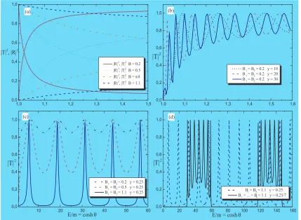
Figure 1: (a) Single defect with varying coupling constant. |T|2
and|R|2
correspond to curves starting at 0 and 1 of the same line type, respectively. (b) Double defect with varying distance y. (c) Double defect with varying effective coupling constant B. (d) Double defect≡ dotted line, eight defects ≡ solid line.
Part (a) of figure 1 confirms the unitarity relation (2.6) where we used R∗j(θ, B) =
Rj(−θ, B) and Tj∗(θ, B) = Tj(−θ, B). Part (b) and (c) show the typical resonances of a double defect, which become stretched out and pronounced with respect to the energy when the distance becomes smaller and the coupling constant increases, respectively. Part (d) ex-hibits a general feature which extends to an even number of higher multiple defects, say 2n, when keeping the distanceybetween the two most separated defects fixed: The resonances ac-cumulate at the position around the (2n−1)-th resonances of the double defect. For increasing
n they become very dense in that region such that one may speak of energy bands.
It is interesting to compare these bands with those obtained from the criterium (2.32), which translates in this case into
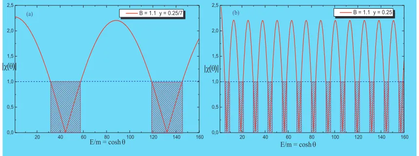
[image:12.612.94.523.173.487.2]Figure 1 part (d) shows that when taking 2n defects separated by a distance y/(2n−1) one obtains for large nan energy spectrum which resembles a band structure. Analyzing instead the functionχαi(θ) in (2.31) we obtain the same band structure from the criterium (2.32). The two computations show that the positions as well as the width of the bands in the two figures 1(d) and 2 coincide quite well. Remarkably, even for the double defect the criterium (2.31) yields energy regions, see figure 2(b), which are in good agreement with the exact computation as presented in figure 1(d).
Figure 2: Band structures according to the criterium (2.32). The non-shaded regions are forbidden. (a) eight defects with B = B1 = . . . = B8 = 1.1 equidistant by y = 0.25/7 (b) double defect with
B=B1=B2= 1.1 distanced byy = 0.25.
Very often we will not be able to perform certain computations analytically, but instead we can carry them out in the massless limit. The prescription for taking this limit was originally introduced in [37]. It consists of replacing in every rapidity dependent expression θby θ±σ, where an additional auxiliary parameter σ has been introduced. Thereafter one should take the limit σ → ∞, m → 0 while keeping the quantity ˆm = m/2 exp(σ) finite. For instance, carrying out this prescription for the momentum yieldsp±=±mˆ exp(±θ), such that one may
view the model as splitted into its two chiral sectors and one can speak naturally of left (L) and right (R) movers. In this way the expressions (2.39)-(2.40) become
Rαj,L/R(θ, B) =±isinB e±2iyαmeˆ θ and Tα
j,L/R(θ, B) = cosB. (2.43) Similarly we compute the expression involving two and four defects for later purposes
Tj,L/Rα1α2(θ, B) = T˜j,L/Rα1α2(θ, B) = cos 2B
1 + sin2Bexp[∓2imˆ(yα1−yα2)eθ]
, (2.44)
Rα1j,L/Rα2 (θ, B) = ±isinB e−2iyα1meˆ θ± isinBcos
2Be−2iyα2meˆ θ
1 + sin2Bexp[∓2imˆ(y
α1−yα2)eθ]
, (2.45)
˜
Rα1j,L/Rα2 (θ, B) = ±isinB e2iyα2meˆ θ ± isinBcos
2Be−2iyα1meˆ θ
1 + sin2Bexp[∓2imˆ(yα1−yα2)eθ]
, (2.46)
Tj,L/Rα1α2α3α4(θ, B) = T˜j,L/Rα1α2α3α4(θ, B) = T α1α2
j,L/R(θ, B)T α3α4 j,L/R(θ, B)
[image:13.612.117.531.561.726.2]The remaining amplitudes can be obtained analogously. The expressions of physical quantities, e.g., the conductance, in the massless limit should not depend on the parameter ˆm, such that the amplitudes (2.43)-(2.47) should in fact always appear in combination with other functions in order to make the prescription meaningful.
Having discussed this type of defect in some detail we will now compute R/R˜ and T /T˜
for various other defects in order to illustrate several types of physical behaviours.
2.3.3 Transparent defects, D0(¯ψ, ψ) = 0, Dβ(¯ψ, ψ) =gψγ¯ 1ψ
The examples which can be handled most easily in later considerations are defects which behave physically as if they were transparent ones, i.e., as |Tα
|= 1. Note that this does not necessarily mean the absence of the defect. For instance considering the defect Dβ(¯ψ, ψ) =
gψγ¯ 1ψ, we compute with the method outlined above
Rβj(θ, B) = ˜Rjβ(θ, B) =R¯β(θ, B) = ˜Rβ¯(θ, B) = 0, (2.48)
Tjβ(θ,−B) = T¯β(θ, B) = ˜T¯β(θ,−B) = ˜Tjβ(θ, B) =eiB, (2.49)
for this defect. The coupling constant is parameterized as in (2.41). Evidently the “unitarity” (2.6)-(2.7) and the crossing relations (2.16)-(2.17) are satisfied. Note that this is also an example for a defect which breaks parity invariance, i.e., the left and right transmission amplitudes are not identical. In the infinite lattice limit, i.e. when the number of defects tends to infinity, we find
χβj/¯(θ) = cos(ky∓B) ⇒ λβj/¯(θ)∈/R,∀θ, B , (2.50) which means that according to (2.29) there are no forbidden energy regimes.
2.3.4 Energy insensitive defects, Dγ(¯ψ, ψ) =gψγ¯ 5ψ, Dδ±(¯ψ, ψ) =gψ¯(γ1±γ5)ψ
In comparison with the transparent defects the next complication arises when the defect causes a phase shift independent of the energy of the incoming particle. For Dγ(¯ψ, ψ) = gψγ¯ 5ψ we compute
Rγj(θ, B,−y) = ˜Rjγ(θ,−B, y) =Rγ¯(θ, B, y) = ˜Rγ¯(θ,−B,−y) =ie2iymsinhθtanB, (2.51)
Tjγ(B) = T¯γ(B) = ˜T¯γ(B) = ˜Tjγ(B) = cos−1(B). (2.52)
In this case we observe that parity is broken for the reflection amplitudes, i.e. R 6= ˜R. The relations (2.6)-(2.7) and (2.16)-(2.17) fory= 0 are satisfied. Fory= 0 none of the amplitudes depend on the rapidities. In the infinite lattice limit we find
χγj(θ) =χγ¯(θ) = coskycosB <1 ∀θ, B , (2.53)
such that according to (2.32) there are no forbidden energy regimes. ForDδ±(¯ψ, ψ) =gψ¯(γ1±γ5)ψ we compute
Rδ±
j (θ, B,−y) = ˜R δ±
j (θ,−B, y) =R δ±
¯
(θ, B, y) = ˜R δ±
¯
(θ,−B,−y) =±itan
B
2e
2iymsinhθ,(2.54)
Tδ±
j (B) = T δ±
¯
(−B) = ˜T¯δ±(B) = ˜Tjδ±(−B) = 1−2itan
B
These are examples in which parity is broken for the reflection as well as for the transmission amplitudes. Again the relations (2.6)-(2.7) and (2.16)-(2.17) are satisfied when the defect is placed at the origin and, as for Dγ, when y = 0 none of the amplitudes depends on the rapidities. In this case we find in the infinite lattice limit
χδ+j/¯(θ) =χδ− j/¯(θ) =
cosky
1∓2itanB2 ⇒ λ δ±
j/¯(θ)∈/R,∀θ, B , (2.56)
such that according to (2.32) there are no forbidden energy regions.
2.3.5 Luttinger liquid type Dε(¯ψ, ψ) = ¯ψ(g1+g2γ0)ψ
When taking the conformal limit of a defect of the typeDε(¯ψ, ψ) = ¯ψ(g
1+g2γ0)ψone obtains an impurity which played a role in the context of Luttinger liquids [38] when setting the bosonic number counting operator to zero, see e.g. [39]. Besides Dα(¯ψ, ψ) this is also an example of a defect for which the potential is real. With (2.34), (2.37) and (2.38) we compute the related transmission and reflection amplitudes
Rεj(θ, g1, g2,−y) = ˜Rεj(θ, g1, g2, y) =
4i(g2+g1coshθ)e2iymsinhθ (4 +g12−g22) sinhθ−4i(g1+g2coshθ)
, (2.57)
Rε¯(θ, g1, g2,−y) = ˜Rε¯(θ, g1, g2, y) =
4i(g1−g2coshθ)e−2iymsinhθ (4 +g2
1−g22) sinhθ−4i(g1−g2coshθ)
, (2.58)
Tjε(θ, g1, g2) = ˜Tjε(θ, g1, g2) =
(4 +g2
2−g12) sinhθ (4 +g2
1 −g22) sinhθ−4i(g1+g2coshθ)
, (2.59)
T¯ε(θ, g1, g2) = ˜T¯ε(θ, g1, g2) =
(4 +g2
2−g21) sinhθ (4 +g2
1 −g22) sinhθ−4i(g1−g2coshθ)
. (2.60)
As we expect, since limg2→0Dε(¯ψ, ψ) = Dα(¯ψ, ψ), we recover the related results also for the
T /T˜’s and R/R˜’s in (2.39)-(2.40). On the other hand, for g1 → 0 we obtain the defect
Dζ(¯ψ, ψ) =g2ψγ¯ 0ψfor which the expressions simplify to
Rζj(θ, B,−y) = ˜Rζj(θ, B, y) = −ie
2iymsinhθsinB
cosBsinhθ+isinBcoshθ, (2.61)
R¯ζ(θ, B, y) = ˜Rζ¯(θ, B,−y) = ie
2iymsinhθsinB
cosBsinhθ−isinBcoshθ, (2.62)
Tjζ(θ, B) = ˜Tjζ(θ, B) =T¯ζ(θ,−B) = ˜T¯ζ(θ,−B) = sinhθ
cosBsinhθ+isinBcoshθ.(2.63)
Where the effective coupling B is given by (2.41) with g → g2. The relations (2.6)-(2.7) and (2.16)-(2.17) may be verified once again for y = 0. In this case the infinite lattice limit leads to forbidden energy regimes, since according to (2.32), the rapidities have to respect the inequality
(4 +g21−g22) sinhθcosky+ sinky(g1±g2coshθ)<(4 +g22−g12) sinhθ forj,¯ , (2.64)
2.3.6 The defects Dη±(¯ψ, ψ) =gψ¯(1±γ5)/2ψ
For this case we compute now
Rη±
j (θ, B, y) = R η±
¯
(θ, B,−y) =
e∓θe−2iymsinhθ
icot(B/2) sinhθ−1, (2.65)
˜
Rη±
¯
(θ, B,−y) = R˜ η±
j (θ, B, y)=
e±θe2iymsinhθ
icot(B/2) sinhθ−1, (2.66)
Tη±
j (θ, B) = T η±
¯
(θ, B) = ˜T η±
¯
(θ, B) = ˜T η±
j (θ, B) =
1
1∓itan−1(B/2) sinh−1(θ),(2.67)
which is once again in agreement with (2.6)-(2.7) and (2.16)-(2.17) for y = 0. In the infinite lattice limit we obtain also in this case forbidden energy regimes. The criterium (2.32) gives
±cosky/2<sinhθtanB/2 sinky/2, (2.68) which has non-trivial solutions for the rapidities.
2.3.7 The defects Dλ±(¯ψ, ψ) =gψ¯(γ0±γ1)/2ψ
For this case we compute now
Rλ±
j (θ, B, y) = R λ±
¯
(θ, B,−y) =
e−2iymsinhθtanB2
isinhθ−tanB2 coshθ, (2.69)
˜
Rλ±
¯
(θ, B, y) = ˜Rλj±(θ, B,−y) =
−e−2iymsinhθtanB2
isinhθ+ tanB2 coshθ, (2.70)
Tλ±
j (θ, B) = T λ±
¯
(θ,−B) = ˜T¯λ±(−θ, B) = ˜Tjλ±(−θ,−B) =
(i±tanB2) sinhθ
isinhθ−tanB2 coshθ.(2.71)
The crossing-hermiticity and unitarity relations hold for y= 0.
In principle we could of course prolong this list of defects and construct their corresponding
R’s andT’s. However, the main purpose of this exercise was to review how the transmission and reflection amplitudes for a defect may be obtained and also to give a brief account of some of their characteristic features. Important to note is that indeed all variations of possible parity breaking occur and one should keep therefore the discussion generic in that sense. Note that when the defect is real, namely Dα(¯ψ, ψ), Dε(¯ψ, ψ), parity invariance is preserved, which is a well known fact from quantum mechanics (see e.g. [34]). Complex potentials might look at first sight somewhat unphysical from the energy spectrum point of view. However, as is well-known for some bulk theories, such as for instance affine Toda field theories with purely complex coupling constants, one can still associate well defined quantum field theories to such Lagrangians and construct even classically soliton solutions with real energies and momenta [40].
A classification scheme for possible defects which maintain integrability is highly desirable. It is interesting to note that in the conformal limit, as outlined before equation (2.43), some of the defects, namely Dζ(¯ψ, ψ) and Dλ±(¯ψ, ψ), become purely transmitting. Therefore, in
3
Conductance from the Landauer formula
3.1 Conductance through an impurity
[image:17.612.182.435.189.352.2]The most intuitive way to compute the conductance is via Landauer transport theory [1]. Let us consider a set up as depicted in figure 3, that is we place a defect in the middle of a rigid bulk wire, where the two halves might be at different temperatures.
Figure 3: A conductance measurement. Part (a) represents the initial condition with no current flowing, i.e., I=0 and part (b),I 6= 0. The defect is placed in the middle of the wire and the left and right half are assumed to be at temperaturesT1andT2, respectively.
The direct currentI through such a quantum wire can be computed simply by determining the difference between the static charge distributions at the right and left constriction of the wire, i.e. I =Qr−Ql. This is based on the assumption [13, 16], thatQ(t)∼(Qr−Ql)t∼(ρr−ρl)t, where theρs are the corresponding density distribution functions. Placing an impurity in the middle of the wire, we have to quantify the overall balance of particles of type i and anti-particles ¯ı carrying opposite charges qi = −q¯ı at the end of the wire at different potentials. This information is of course encoded in the density distribution function ρr
i (θ, T, µi). In the described set up half of the particles of one type are already at the same potential at one of the ends of the wire and the probability for them to reach the other is determined by the transmission and reflection amplitudes through the impurity. We assume that there is no effect coming from the constrictions of the wire, i.e. they are purely transmitting surfaces with T = ˜T = 1. One could, however, also consider a situation in which those constrictions act as boundaries, namely purely reflecting surfaces. The situation could be described with the same transport theory picture, see e.g. [13, 14, 41], but then the conductance can only be non-vanishing if the reflection amplitudes in the constrictions are non-diagonal in the particle degrees of freedom, such as for instance for sine-Gordon [29], that is in general affine Toda field theories with purely imaginary coupling constant or in the massless limit folded purely reflecting (transmitting) diagonal bulk theories.
According to the Landauer transport theory the direct current (DC) along the wire is given by
Iα
= X
i
Iα
i (r, µli, µri) = X
i
qi 2
∞
Z
−∞
dθhρri(θ, r, µri)|Tα
i (θ)|2−ρir(θ, r, µli)|T˜ α i (θ)|2
i
= IB− X
i
qi 2
∞
Z
−∞
dθhρri(θ, r, µri)|Rα
i (θ)|2−ρir(θ, r, µli)|R˜ α i (θ)|2
i
, (3.2)
where we assume here T1 = T2. The relation (3.2) is obtained from (3.1) simply by making use of the fact that |R|2 +|T|2 = 1. Equation (3.2) has the virtue that it extracts explicitly the bulk contribution to the current which we refer to as IB. There are some obvious limits, namely a transparent and an impenetrable defect
lim
|Tα|→1
Iα
=IB and lim
|Tα|→0
Iα
= 0, (3.3)
respectively. A short comment is needed on the validity of (3.1). Apparently it suggests that when the parity between left and right scattering is broken, there is the possibility of a net current even when an external source is absent. In this picture we have of course not taken into account that charged particles moving through the defect will alter the potential, such that we did in fact not describe a perpetuum mobile. Thus the limitation of our analysis is that µl
i−µri has to be much larger than the change in the potential induced by the moving particles.
Finally we want to compute the conductance from the DC current, which by definition is obtained from
Gα
(r) =X iG
α i (r) =
X
i(µllim i−µri)→0
Iα
i (r, µli, µri)/(µli−µri) (3.4)
and is of course a property of the material itself and a function of the temperature. In general the expressions in (3.1) tend to zero for vanishing chemical potential difference such that the limit in (3.4) is non-trivial.
Thus from the knowledge of the transmission matrix and the density distribution function we can compute the conductance. Having already described how Tα
i (θ) can be determined, we will now explain how ρri(θ, r, µi) can be evaluated by exploiting the integrability of the theory.
3.2 Defect TBA equations
The thermodynamic Bethe ansatz is a powerful tool which may be used to compute various thermodynamic properties of multi-particle systems which interact via a factorizing scattering matrix [9] and some chosen statistics. In addition, it allows to check the theory for consistency and to extract some distinct structural quantities such as the Virasoro central in the ultraviolet limit. The original bulk formulation has been accommodated to a situation which includes a purely transmitting defect [42] and a boundary [44]. In this section we want to propose a new formulation which is valid for a situation not treated before in this context, namely when reflection and transmission occur simultaneously.
As usual we obtain the Bethe ansatz equation by dragging a particle along the world line of length L. We introduce for convenience the following shorthand notation for the product of various particle Zi(θ) and defect operators Zα
Zµ1...µN
Then we compute the braiding of a particle operator of type i and the product ofN further particlesZµ1. . . ZµN with one defectZα situated on the right of the particleZµk by using the
ZF-algebra (2.3) and (2.4)
Zi(θi)Zk,αµ1...µN = Z µ1...µN
k,α Zi(θi) ˜Fiα−Zk,αµ1...µNZi(−θi) ˜Giα, (3.6)
Zµ1...µN
k,α Zi(θi) = Zi(θi)Z µ1...µN
k,α Fiα−Zi(−θi)Z µ1...µN
k,α Giα. (3.7)
We abbreviated here
˜
Fiα = 1 ˜
Tiα(−θi) N Y l=1
Siµl(θiµl), G˜
α i =
˜
Rα i(−θi) ˜
Tiα(−θi) k Y l=1
Siµl(θiµl)
N Y l=k+1
Siµl(−ˆθiµl), (3.8)
Fiα = 1
Tiα(θi) N Y l=1
Sµli(θµli), G
α i =
Rα i(θi)
Tiα(θi) k Y l=1
Sµli(ˆθµli)
N Y l=k+1
Sµli(θµli) . (3.9)
Being on a circle of length L, we can make the usual assumption on the Bethe wavefunction, see e.g. [9], which is captured in the requirement
Zi(θ)Zk,αµ1...µN =Z µ1...µN
k,α Zi(θ) exp(−iLmisinhθ). (3.10)
Using this monodromy property together with the braiding relations (3.6), (3.7) and the unitarity relation (2.6), we obtain
N Y l=1
Sli(ˆθli)
Sli(θli) N Y l=1
Sli(θli)−
eiLmisinhθi
˜
Tα i (−θi)
! = T
α i (−θi) ˜
Tα i (−θi)
e−iLmisinhθi Tα
i (θi) − N Y l=1
Sil(θil) !
. (3.11)
Viewing the subscripts as entire spaces rather than components, equation (3.11) corresponds to the Bethe ansatz equation with simultaneously occurring transmission and reflection am-plitudes for the generic, that is also the non-diagonal, case. We restrict it here to the diagonal case and can therefore use the constraints (2.15), such that the bulk scattering matrix becomes rapidity independent and the relation (3.11) may be re-written as
1 =eiLmisinhθD±
iα(θ)
YN
l=1Sil (3.12)
where
Diα±(θ) = T˜ α
i (θ) +Tiα(θ) QN
l=1Sil2
2 ±
1 2
T˜iα(θ) +Tiα(θ) N Y l=1
Sil2
!2
− 4T
α i (θ)
QN l=1Sil2
Tα i (−θ)
1 2 . (3.13) For consistency reasons it is instructive to consider the limit when the reflection amplitude tends to zero. In that case we can employ the relations (2.5)-(2.7) and may take the square root in (3.13), such that we obtain from (3.12) the two equations
R,R˜→0 : 1 =eiLmisinhθT˜α
i (θ) N Y l=1
Sil, 1 =e−iLmisinhθTiα(θ) N Y l=1
This means we recover the Bethe ansatz equations for a purely transmitting defect, which were originally proposed by Martins in [42]. The two signs in (3.13) capture the breaking of parity invariance in the limiting case, i.e. the two equations in (3.14) correspond to taking the particle either clockwise or anti-clockwise around the world line as formulated for the parity breaking case for the first time in [43]. We do not expect to recover from here the equations for a purely reflecting boundary which were suggested in [44], since the equations (3.6) and (3.7) do not make sense in the limit T,T˜→0. ForQN
l=1Sil2 = 1,i.e. the free Boson and Fermion, we can exploit the fact that (3.12) with (3.13) look formally precisely like the Bethe ansatz equations for a purely transmitting defect. If we want to exploit this analogy we should of course be concerned about the question whetherD±jα(θ) is a meromorphic function. Assuming parity invariance, we may take the square root
Djα±(θ) =Tjα(θ) ±Rjα(θ) for T = ˜T , R= ˜R . (3.15)
The matrix Djα±(θ) has now the usual properties, namely it is unitarity in the sense that
D±jα(θ)D±jα(−θ) = 1. It follows further from (3.15), (2.16) and (2.17) that the hermiticity relation Djα±(θ) =Djα±(−θ)∗ and the crossing relations D±
¯
α(θ) = Djα∓(iπ−θ) and D±¯α(θ) =
D±jα(iπ−θ) hold for the free Fermion and Bosons, respectively.
Let us now carry out the thermodynamic limit in the usual way, namely by increasing the particle number and the system size in such a way that their mutual ratio remains finite. The amount of defects is kept constant in this limit, such that there is no contribution to the TBA-equations from the defect in that situation, see also [42] where the same argument was employed. Hence this means that essentially we can employ the usual bulk TBA analysis when the considerations are carried out not per unit length.
Let us therefore recall the main equations of the TBA analysis. For more details on the derivation see [9] and in particular for the introduction of the chemical potential see [10]. The main input into the entire analysis is the dynamical interaction, which enters via the logarithmic derivative of the scattering matrix ϕij(θ) =−idlnSij(θ)/dθ and the assumption on the statistical interaction, which we take to be fermionic. As usual [9, 10], we take the logarithmic derivative of the Bethe ansatz equation (3.12) and relate the density of states
ρi(θ, r) for particles of typeias a function of the inverse temperaturer= 1/T to the density of occupied states ρri(θ, r)
ρi(θ, r) = mi
2π coshθ+
X
j[ϕij ∗ρ r
i](θ). (3.16)
By (f∗g) (θ) := 1/(2π)R
dθ′f(θ−θ′)g(θ′) we denote as usual the convolution of two functions. The mutual ratio of the densities serves as the definition of the so-called pseudo-energies
εi(θ, r)
ρri(θ, r)
ρi(θ, r) =
e−εi(θ,r)
1 +e−εi(θ,r), (3.17)
which have to be positive and real. At thermodynamic equilibrium one obtains then the TBA-equations, which read in these variables and in the presence of a chemical potential µi
rmicoshθ=εi(θ, r, µi) +rµi+ X
j[ϕij∗ln(1 +e
where r =m/T,ml →ml/m,µi →µi/m, with m being the mass of the lightest particle in the model. It is important to note that µi is restricted to be smaller than 1. This follows immediately from (3.18) by recalling that εi ≥ 0 and that for r large εi(θ, r, µi) tends to infinity. As pointed out already in [9] (here just with the small modification of a chemical potential), the comparison between (3.18) and (3.16) leads to the useful relation
ρi(θ, r, µi) = 1 2π
dεi(θ, r, µi)
dr +µi
. (3.19)
The main task is therefore first to solve (3.18) for the pseudo-energies from which then all densities can be reconstructed.
3.3 Thermodynamic quantities
Treating the equations (3.12) and (3.13) in the mentioned analogy we can also construct various thermodynamic quantities. It should be stressed that these quantities are computed per unit length. Similarly as the expression found in [42] for a purely transmitting defect the free energy is
F(r) =− 1
πr
X l,α
ˆ
ml
Z ∞
0
dθ[coshθ+m−1ϕlα(θ)] ln[1 + exp(−rmcoshθ)]. (3.20)
It is made up of two parts, one coming from the bulk and one including the data of the defect in form of ϕlα(θ) = −idlnDlα(θ)/dθ. From equation (3.20) we also see that when taking the mass scale to be large in comparison to the dominating scale in the defect, the latter contribution to the scaling function becomes negligible with regard to the bulk and vice versa.
3.4 The high temperature regime
Since the physical quantities require a solution of the TBA-equations, which up to now, due to their non-linear nature, can only be solved numerically, we have to resort in general to a numerical analysis to obtain the conductance for some concrete theories. However, there exist various approximations for different special situations, such as the high temperature regime. For large rapidities and small r, it is known [9] (here we only need the small modification of the introduction of a chemical potential µi) that the density of states can be approximated by
ρi(θ, r, µi)∼ mi 4πe
|θ|∼ 1
2πrǫ(θ)
dεi(θ, r, µi)
dθ , (3.21)
where ǫ(θ) = Θ(θ)−Θ(−θ) is the step function, i.e. ǫ(θ) = 1 for θ > 0 and ǫ(θ) = −1 for
θ <0. In equation (3.17), we assume that in the large rapidity regimeρri(θ, r, µi) is dominated by (3.21) and in the small rapidity regime by the Fermi distribution function. Therefore
ρri(θ, r, µi)∼ 1 2πrǫ(θ)
d
dθ ln [1 + exp(−εi(θ, r, µi))] . (3.22)
Using this expression in equation (3.1), we approximate the direct current in the ultraviolet by
lim r→0I
α
i (r, µi)∼
qi 4πr
∞
Z
−∞
dθln
1 + exp(−εi(θ, r, µli)) 1 + exp(−εi(θ, r, µri))
dǫ(θ)
|Tα i (θ)|2
after a partial integration. For simplicity we also assumed here parity invariance, that is
|Tα
i (θ)|=|T˜ α
i (θ)|. The derivation of the analogue to (3.23) for the situation when parity is broken is of course similar. Taking now the potentials at the end of the wire to beµri =−µli =
V /2, the conductance reads in this approximation
lim r→0G
α i (r)∼
qi 2πr ∞ Z −∞ dθ 1
1 + exp[εi(θ, r,0)]
dεi(θ, r, V /2)
dV V=0 d
ǫ(θ)|Tα i (θ)|2
dθ . (3.24)
In order to evaluate these expressions further, we need to know explicitly the precise form of the transmission matrix, i.e. the concrete form of the defect. An interesting situation occurs when the defect is transparent or rapidity independent, that is|Tα
i (θ)| → |T α
i |, in which case we can pursue the analysis further. Noting that dǫ(θ)/dθ= 2δ(θ), we obtain
lim r→0G
α i (r)∼
qi
πr
|Tα i |2 1 + expεi(0, r,0)
dεi(0, r, V /2)
dV V=0 . (3.25)
The derivative dεi(0, r, V /2)/dV can be obtained by solving recursively
dεi(0, r, V /2)
dV =− r 2 − X j Nij 1
1 + expεj(0, r, V /2)]
dεj(0, r, V /2)
dV , (3.26)
which results form a computation similar to a standard one in this context [9] leading to the so-called constant TBA-equations. Here only the asymptotic phases of the scattering matrix enter viaNij = limθ→∞[ln[Sij(−θ)/Sij(θ)]]/2πi. The values of εi(0, r,0) needed in (3.25) can be obtained for small r in the usual way from the standard constant TBA-equations.
3.5 Free Fermion with defects
Let us exemplify the general formulae once more with the free Fermion. First of all we note that in this case in the TBA-equations (3.18) the kernel ϕij is vanishing and the equation is simply solved by
εi(θ, r, µi) =rmicoshθ−rµi. (3.27)
Therefore, we have explicit functions for the densities with (3.19) and (3.17)
ρi(θ, r, µi) = 1
2πmicoshθ and ρ
r
i(θ, r, µi) =
micoshθ/2π 1 + exp(rmicoshθ−rµi)
. (3.28)
According to (3.1) the direct current reads
Iα
(r, V) = qi 2
∞
Z
−∞
dθ
ρr¯ı (θ, r, V /2)|Tα
¯ı (θ)|2−ρri(θ, r,−V /2)|T α i (θ)|2
−ρ¯rı (θ, r,−V /2)|T˜α
¯ı (θ)|2+ρri (θ, r, V /2)|T˜ α i (θ)|2
i
. (3.29)
Using atomic units me=e=h=mi=qi = 1, we obtain explicitly with (3.28)
Iα
(r, V) = 1
π
∞
Z
0
dθcoshθsinh(rV /2)|T
α
(θ)|2
for |Tα
¯ı (θ)| = |T α
i (θ)| = |T˜ α
¯ı (θ)| = |T˜ α
i (θ)| = |T α
(θ)|. Then by (3.4) the conductance results to
Gα
(r) =rme
2
h
∞
Z
0
dθ coshθ |T
α
(θ)|2
1 + cosh(rmcoshθ) (3.31)
in this case. We have re-introduced dimensional quantities instead of atomic units to be able to match with some standard results from the literature. The most characteristic features can actually be captured when we carry out the massless limit as indicated in section 2.3.2, which can be done even analytically. Substituting t=eθ, we obtain
lim m→0G
α
(r)∼ e 2
h
∞
Z
0
dt|T
α
L/R(t y/r)|2 1 + cosh(t) =
e2 h
(
|Tα
L/R(t y/r)|2 fory≫r
|Tα
L/R(y/r = 0)|2 fory≪r
. (3.32)
We have identified here two distinct regions. When y ≪ r we can replace the left/right transmission amplitudes by their values aty/r = 0. Wheny ≫rthe transmission amplitudes enter the expression as a strongly oscillatory function in which y/r plays the role of the frequency. It is then a good approximation to replace this function by its means value as indicated by the overbar. It is straightforward to extend the expression (3.32) to the case when the assumption on Tα
in (3.30) is relaxed and to the case with different values of y. To proceed further we need to specify the defect.
3.5.1 Energy insensitive defects, D0(¯ψ, ψ) = 0, Dβ(¯ψ, ψ), Dγ(¯ψ, ψ), Dδ±(¯ψ, ψ)
Let us first consider the easiest example, which supports the general working of the method. When the defect is transparent, i.e., |Tα
| = 1, we can compute the expression for the con-ductance (3.31) directly in the large temperature limit and obtain the well known behaviour [45]
lim r→0,|Tα
|→1G
α
(r)∼ e 2
h(1− rm
2 ). (3.33)
Alternatively we obtain the expression (3.33) also from equation (3.25) and (3.27). In the massless limit of (3.32) we obtain e2/hwhich coincides with the result in [13]. However, we should stress that we consider here purely massive cases and the massless limit only serves as a benchmark. Note that a transparent defect in this context does not necessarily mean the absence of the defect. Considering for instance the defect Dβ(¯ψ, ψ), we compute with (2.48) and (2.49) the same conductance as if there was no defect at all. Similarly simple are the computations for the defects Dγ(¯ψ, ψ),Dδ±(¯ψ, ψ). We simply get
G0(r) =Gβ(r) =Gγ(r) cos2B =Gδ±(r)/(1 + 4 tan2B/2) = e
2
h. (3.34)
Since the amplitudes do not depend on the rapidities, the TBA-kernel is zero and there is no contribution from this defect to the free energy, even unit length.
3.5.2 The energy operator defect Dα(¯ψ, ψ) =gψψ¯
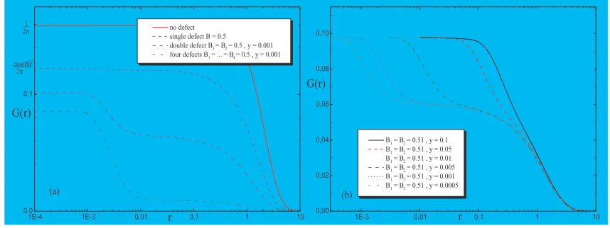
Figure 4: Conductance G(r) for the complex free Fermion with the energy operator defects as a function of the inverse temperature r, for fixed effective coupling constant B and (a) for varying amounts of defectsℓ= 0,1,2,4. (b) forℓ= 2 for varying distancesy.
We observe several distinct features. First of all it is naturally to be expected that when we increase the number of defects the resistance will grow. This is confirmed, as for fixed temperature and increasing number of defects, the conductance decreases. Second we see several well extended plateaux. They can be reproduced with the analytical expressions obtained in the massless limit (3.32). To be able to compare with (3.31) we re-introduce atomic units for convenience, i.e. e2/h→1/2π. For a single defect there is only one plateaux and from (3.32) we obtain with (2.43)
Gα(r)∼ cos 2B
2π . (3.35)
For B = 0.5 the value 0.1226 is well reproduced in figure 4(a). The lower lying plateaux correspond to the region when y ≪ r. In that case we obtain from (3.32) together with the expressions (2.44)-(2.47) for a double and four defects
Gα1α2(r) ∼ 1 2π
cos2B
1 + sin2B
2
for y≪r , (3.36)
Gα1α2α3α4(r) ∼ 1 2π
cos4B
cos4B−2(1 + sin2B)2 2
fory≪r. (3.37)
For B = 0.5 the values 0.0624 and 0.0095 are well reproduced in figure 4(a) for ℓ = 2 and
ℓ= 4, respectively. The plateaux extending to the ultraviolet regime result from (3.32) and by taking in (2.44)-(2.47) the mean values
Gα1α2(r) ∼ 2
π
1 + sin4B
(cos2(2B)−3)2 , fory ≫r , (3.38)
Gα1α2α3α4(r) ∼ 1 4π +
cos8B
4π[cos4B−2(1 + sin2B)2]2, fory≫r. (3.39)
reason for the increase from one to the next plateaux and why the curves are shifted precisely in the way as indicated in figure 4(b) when we change the distance between the defects. This phenomenon is attributed to resonances as we shall discuss in more detail in the next subsection.
3.5.3 Resonances versus unstable particles
In [46] we demonstrated that resonances may be described similarly as unstable particles. The latter provide an intuitively very clear picture which explains the relatively sharp onset of the conductance with increasing temperature. The temperature at which this onset occurs, sayTC can be attributed directly to the energy scale at which the unstable particle is formed, since then it starts to participate in the conducting process. The Breit-Wigner formula [47] constitutes in this case a relation for the massM and the decay width Γ of an unstable particle. Supposing that in the scattering process between particles of typeiandjan unstable particle can be formed, this is reflected by a pole inSij(θ) atθ=σ−iσ¯. Then, for large values of the resonance parameter σ one may approximate
M2≈1/2mimj(1 + cos ¯σ) exp|σ| and Γ2 ≈2mimj(1−cos ¯σ) exp|σ|. (3.40)
Since a renormalization group flow is provided by M → r M, one should observe that the quantities M ∼r1eσ1/2 =r2eσ2/2 and Γ∼ r1eσ1/2 =r2eσ2/2 remain invariant. Accordingly, this creation of the unstable particle should be reflected in the conductance as
G(r1, σ1) =G(r2, σ2) for r1eσ1/2=r2eσ2/2. (3.41)
This means we can control the position of the onset in the conductance byM and its extension in the temperature direction by Γ. For a model which possesses unstable particles we found indeed such a behaviour [46]. From the data of the previous subsections we find that the conductance scales as G(r1, y1) =G(r2, y2) forr2y1 =r1y2. Then the comparison with (3.41) suggests that we can relate the distance between the two defects to the resonance parameter as σ = 2 ln(const/y). From the maxima in |T(θ)| we may identify various σs and in fact in this case the net result can be attributed to two resonances [46].
3.5.4 Multiple plateaux
Up to now, we have observed that we always obtain essentially two plateaux in the conduc-tance, no matter how many (≥ 2) and what type of defects we implement. The natural question arising at this point is whether it is possible to have a set up which leads to a more involved plateaux structure? It is clear that if we had many defects in a row separated far enough from each other such that the relaxation time of the passing particles is so large that they could be treated as single rather than multiple defects, then any desired type of multiple plateau structure could be obtained. In this case the conductance is simply the sum of the ex-pressions one has for each defect independently. Recalling the origin of the different plateaux, there is another slightly less obvious option. The density distribution function ρr is a peaked function of the rapidity and if the resonances in Tα
of the resonances in the rapidity variable or change their amplitudes, respectively (see section 2).
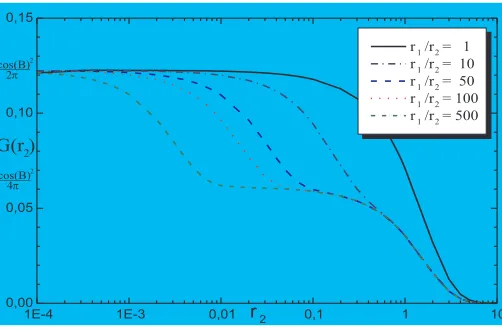
Figure 5: Conductance G(r2) for the complex free Fermion with the energy operator defects as a
function of the inverse temperature r2, for fixed effective coupling constant B = 0.5 and varying
temperature ratios in the two halves of the wire.
Therefore the last option left is to change theρrs, which is possible by varying the temperature. Choosing now a configuration as in figure 3 with different temperatures T1 and T2, one can “create” a second plateau at half the height of the original one. The reason for this is simply that the cooled half of the wire will cease to contribute to the conductance as can be directly deduced from (3.31). We depict the results of our computations in figure 5.
From this it also obvious that if we only cool the fraction x of the wire, the lowest plateau will be positioned at the height xtimes the height of the upper plateau. Thus, by combining these different configurations, i.e., different temperatures or defects, we could produce any desired plateau structure.
4
Conductance from the Kubo formula
Having computed the DC conductance by means of a TBA analysis, we want to proceed now by introducing an alternative method for the acquisition of the same quantity, that is the evaluation of the celebrated Kubo formula‡[3]
G(T) =−lim ω→0
1 2ωπ2
∞
Z
−∞
dt eiωt hJ(t)J(0)iT,m. (4.1)
The key quantity needed for the explicit computation of (4.1) is the occurrence of the current-current correlation functionhJ(r)J(0)iT,m. In the latter, the subscripts (T,m) indicate that, in general, one is interested in a situation when both, the mass scale of the particles in the quantum field theory and the temperature, are non-vanishing. This is precisely the same regime in which we have carried out the TBA analysis in the previous section and ultimately