A high order compact scheme for hypersonic aerothermodynamics

A High Order Compact Scheme for Hypersonic

Aerothermodynamics

Vincenzo Fico

_{, David R. Emerson}

_{and Jason M. Reese}

a _{STFC Daresbury Laboratory, Warrington WA4 4AD, UK}

b _{University of Strathclyde, Glasgow G1 1XJ, UK}

A novel high order compact scheme for solving the compressible Navier-Stokes equations has been developed. The scheme is an extension of a method originally proposed for solving the Euler equations, and combines several techniques for the solution of compressible flow fields, such as upwinding, limiting and flux vector splitting, with the excellent properties of high order compact schemes. Extending the method to the Navier-Stokes equations is achieved via a Kinetic Flux Vector Splitting technique, which represents an unusual and attractive way to include viscous effects. This approach offers a more accurate and less computationally expensive technique than discretizations based on more conventional operator splitting. The Euler solver has been validated against several inviscid test cases, and results for several viscous test cases are also presented. The results confirm that the method is stable, accurate and has excellent shock-capturing capabilities for both viscous and inviscid flows.

I.

Introduction

Access to Earth or planetary orbits, and entry into the Earth’s atmosphere, require flight through the hy-personic regime. This flight regime often proves to be the design driver for most of the vehicle’s systems and components. Today, the state-of-the art for hypersonic flow simulations consists of a second order discretiza-tion, shock-capturing schemes on structured grids with some limited capabilities on unstructured grids. Two common problems of codes employing these kind of methods are: 1) high levels of dissipation making them poor candidates for Large Eddy Simulation (LES); and 2) inadequate grid convergence properties. Without doubt, there is great interest in designing robust and reliable high order and high resolution methods suitable for hypersonic flow simulation. Compact algorithms make it possible to devise, on a given stencil, difference schemes that have much better spatial resolution properties than conventional explicit difference schemes of comparable order of accuracy, and more compact stencils.

When a wide range of spatial scales and structures has to be computed, spectral and pseudo-spectral schemes are commonly used. Compact schemes with spectral-like resolution properties are more convenient to use than spectral and pseudo-spectral schemes, and are easier to handle, especially when complex geometries are involved. The price paid is that one is required in general to invert a block tridiagonal system of linear equations to obtain derivatives.

The interest in compact schemes started with the pioneering work by Lele,1 _{even though compact} ap-proximations had been used previously by other authors. The first compact schemes developed were central schemes. However, centered algorithms are intrinsically non-dissipative and cannot prevent odd-even de-coupling, which gives rise to high frequency oscillations even in smooth regions. Asymmetric schemes, with their dissipative properties, are more stable. However even asymmetric compact schemes cause non-physical oscillations when applied directly to flows with discontinuities. These non-physical oscillations (Gibbs phe-nomena) do not decay in magnitude even if the grid is refined. Several methods have been proposed to stabilize compact schemes when resolving flows with discontinuities. These methods belong to one of the following three categories.

∗_{Ph.D. student, [email protected]}

The first class are those proposed by Cook and Cabot,2, 3_{Fiorina and Lele}4_{and Cook.}5 _{Very high order} background dissipation terms are added to a central scheme. These artificial dissipation terms are related to very high order derivatives so that the error introduced is smaller than the truncation error of the scheme. This strategy is by far the most accurate, as one has full control of the amount of dissipation introduced, just sufficient to capture discontinuities and damp unphysical oscillations. Drawbacks of this strategy are: (i) the fine tuning required for the artificial diffusivity coefficients; (ii) its complexity; (iii) the loss of the compactness of the stencil, because of the very high order derivatives in the artificial dissipation terms.

In the second class are methods which blend the compact scheme with an essentially non-oscillatory scheme, such as ENO/WENO6–8_{schemes. Compact and ENO/WENO schemes have complementary} prop-erties: compact schemes have excellent resolution properties but oscillatory behavior near discontinuities; ENO/WENO schemes are non-oscillatory but dissipative even for intermediate wavenumbers, and are un-satisfactory in smooth regions with moderately high field gradients. By switching from a compact to a ENO/WENO scheme near discontinuities one can achieve uniformly high accurate solutions with high res-olution in smooth regions and non-oscillatory behavior in regions with steep gradients. However, a free threshold parameter, which controls the switch between the compact and the ENO/WENO scheme, needs to be tuned, and some of these hybrid schemes9, 10 _{experience non-smooth transition near the interface where} the scheme switches types. Spurious waves will eventually propagate into the smooth regions, as reported by Adams and Shariff.10 _{Ren et al.}11 _{have developed a characteristic-wise hybrid scheme, which can be} regarded as an improvement of the method proposed by Pirozzoli.9

Methods belonging to the third category rely on a classical limiting strategy. Cockburn and Shu12_have developed a non-linear limiter to avoid spurious oscillations while maintaining the formal accuracy of the scheme. However, in their numerical tests, spurious oscillations were still evident. Yee13 _{extended and} improved the latter scheme, but no numerical tests were given. Ravichandran14 _{employed a TVD limiter} combined with a kinetic flux vector splitting (KFVS) method to improve stability of compact upwind schemes, proposing a third order scheme supposed to degenerate to first order accuracy at the extrema. Recently Tu and Yuan15 _{proposed a method where a compact upwind scheme is limited through a characteristic-based} approach. The limiting approach is not as common as the hybridizing approach, as degeneration of accuracy near extrema is an undesirable feature when solving, for example, shock-turbulence interaction problems. Furthermore, Cockburn and Shu12 _{found that the introduction of minmod limiters in centered schemes} affects the accuracy of the solution, even in smooth regions, if there are spurious oscillations to suppress. On the other hand, Ravichandran14_{showed that upwinding the compact scheme and employing kinetic splitting} provide effective damping of spurious oscillations in smooth regions, and thus the accuracy degenerates only across discontinuities. This approach is attractive also for its relative simplicity, robustness, and lower computational cost.

We have selected the scheme proposed by Tu and Yuan15 _{as a solution method to extend and improve.} The compact scheme employed has been proposed by Pirozzoli9 _{and has some very interesting features.} First, it is upwind and is derived with a conservative approach, so it is suitable for problems involving discontinuities. Moreover, only the inversion of a tridiagonal system of equations is required, hence it is not as computationally demanding as other compact schemes. Finally, an extensive analysis of the scheme has been conducted,9_{showing its excellent resolution and spectral properties. Tuet al.}16 _{proposed a TVD limiter} and have applied it to the compact scheme developed by Pirozzoli. Tu and Yuan15 _{have also proposed a} characteristic-based treatment for the resulting compact TVD scheme: applying the limiting function to the characteristic variables allows tighter control of the spurious oscillations near discontinuities. The algorithm proposed by Tu and Yuan15 _{is very promising for compressible fluid dynamics, in particular for hypersonic} problems: it has excellent shock-capturing properties because of the conservative approach in deriving the compact scheme; it is stable for problems involving strong discontinuities, such as hypersonic flow fields, because of the upwinding and the limiter function; it is highly accurate in a narrow stencil because of the compact algorithm, but it is not computationally demanding because only a tridiagonal system of linear algebraic equations has to be inverted.

II.

Governing Equations

The governing equations are the Navier-Stokes equations, whose conservative vector form is:

∂Q ∂t +

∂(E+Ev) ∂x +

∂(F+Fv) ∂y +

∂(G+Gv)

∂z = 0, (1)

where Q=              ρ ρu ρv ρw ρE             

, E=              ρu ρu2_+p

ρuv ρuw ρuH             

, F =              ρv ρvu ρv2_+p

ρvw ρvH             

, G=              ρw ρwu ρwv ρw2_+p

ρwH              ,

Ev=

                   0

−τx,x

−τx,y

−τx,z

−τx,xu−τx,yv−

τx,zw+qx

                  

, Fv=

                   0

−τy,x

−τy,y

−τy,z

−τy,xu−τy,yv−

τy,zw+qy

                  

, Gv=

                   0

−τz,x

−τz,y

−τz,z

−τz,xu−τz,yv−

τz,zw+qz

                   .

The stress tensorτ and the heat flux vectorqare:

τ= 

 

τx,x τx,y τx,z τy,x τy,y τy,z τz,x τx,y τz,z





=µ(∇V +∇V

T₎₋2

3µ(∇ ·V)I, q=      qx qy qz     

=−cpµ P r∇T.

In the above equations, ρ is the mass density, V the velocity vector, u, v and w its components along x, y and z directions, respectively, p the pressure, T the temperature, H the total enthalpy, µ the viscosity, P r the Prandtl number, cp the constant pressure specific heat,I the identity tensor and the superscriptT denotes tensor transposition.

III.

Numerical Method

In this section we first describe the inviscid solver we use as a building block for our viscous solver. We consider different versions of the method and then discuss its extension to viscous flows.

A. The solution method for the Euler equations

In this section we outline the scheme proposed by Tu and Yuan15 _{to solve the Euler equations. Consider a} hyperbolic system of one-dimensional conservation laws:

∂Q ∂t +

∂E(Q)

∂x = 0, (2)

whose non-conservative form is:

∂Q ∂t +A

∂Q ∂x = 0,

whereA=dE/dQis the flux Jacobian matrix, which, as the system is hyperbolic, has real eigenvalues and a full set of linearly independent eigenvectors. It can be decomposed as follows:

A=RΛL,

The semi-discrete form of Eq. (2) is:

∂Qi ∂t +

Hi+1/2−Hi−1/2

∆x = 0, i= 1,2, . . . , N,

where Hi+1/2 is the numerical flux function which is split into its positive and negative parts Hi+1/2 = H_i+_+1/2+H_i−_+1/2, and calculated as the sum of a first order term and a high order correction:

H+

i+1/2=E + i +φ

+

i+1/2, H

−

i+1/2=E

−

i+1−φ

−

i+1/2.

In the above relations E± _{can be any splitting of the flux vector E. The classical Steger-Warming flux} vector splitting was employed by Tu and Yuan.15 _{The high order correctionφ}±_{is calculated as follows. The} positive part of the high order numerical flux function ˆE_i+_+1/2 is calculated solving the following tridiagonal system of linear algebraic equations:

ˆ

E₁+_/2 = 1 4E + 0 + 13 12E + 1 − 5 12E + 2 + 1 12E + 3,

9 ˆE+

i−1/2+ 18 ˆE +

i+1/2+ 3 ˆE +

i+3/2 = E +

i−1+ 19E + i + 10E

+

i+1, i= 1, . . . , N,

ˆ

E_N+_+1/2 = 25 12E + N − 23 12E + N−1+

13 12E

+ N−2−

1 4E

+ N−3.

The scheme to compute the negative part of the high order numerical flux function ˆE−_i+1/2 can be obtained from the scheme above by symmetry considerations, and reads:

ˆ

E₁−_/2 = 25 12E − 1 − 23 12E − 2 + 13 12E − 3 − 1 4E − 4,

3 ˆE_i−_−1/2+ 18 ˆE_i−_+1/2+ 9 ˆE_i−_+3/2 = 10fi−+ 19Ei−+1+E

−

i+2, i= 1, . . . , N,

ˆ

E_N−_+1/2 = 1 4E

−

N+1+ 13 12E − N − 5 12E −

N−1+ 1 12E

−

N−2.

Following the component-wise reconstruction of the positive and negative high order numerical flux function ˆ

E_i±+1/2, the flux increments are computed and projected along characteristic directions:

∆ ˆW+

i+1/2=L l_{( ˆE}+

i+1/2−E +

i ), ∆W +

i+1/2=L l_(E+

i+1−E + i ),

∆ ˆW_i−_+1/2=Lr(E_i−+1−Eˆ

−

i+1/2), ∆W

−

i+1/2=L r_(E−

i+1−E

−

i ).

The left eigenvector matricesLl_andLr _{can be evaluated in either of the following ways:}

1. Upwind evaluation,i.e._,Ll_{=L(Qi) andL}r_=L(Qi+1).

2. Evaluation at the Roe average stateQRoe

i+1/2betweenQi andQi+1,i.e.,L

l_=Lr_=L(QRoe i+1/2).

The upwind evaluation was preferred by Tu and Yuan,15 _{as it was expected to be more dissipative and thus} more stable. We have considered both evaluations; a comparison will be shown in SectionIV. We note that ∆ ˆW_i±_+1/2 and ∆W_i±_+1/2 are, respectively, high and low order upwind evaluations of the spatial increment of fluxes of the characteristic variables. They are limited according to:

δW+

i+1/2 = φ(∆ ˆW +

i+1/2,∆W +

i+1/2,∆W + i−1/2),

δW_i−_+1/2 = φ(∆ ˆW_i−_+1/2,∆W_i−_+1/2,∆W_i−_+3/2).

The limiterφcan be either of the following functions:16

φA(a, b, c) = (

sgn(a) min(|a|,|b|), ifa, b, chave the same sign,

0, otherwise.

φB(a, b, c) = (

sgn(a) min|a|,|b|, 2bc

|a|+|c|+ǫ

, ifa, b, chave the same sign,

whereǫis an arbitrary small constant to avoid division by zero. Note that the type A limiter is a version of the well known minmod limiter, whilst type B is a combination of the latter limiter and a version of the van Leer limiter. Finally, the correctionφ±_i+1/2is calculated by projecting the limited increment of characteristic fluxes back into conserved variable space:

φ+_i+1/2=RlδW_i+_+1/2, φ−_i+1/2=RrδW_i−_+1/2,

whereRl _andRr _{are right eigenvector matrices, whose evaluation is such that they are consistent with the} left eigenvector matricesLl _{and L}r_{, respectively. The time derivative in Eq. (2) is discretized via a third} order Runge-Kutta scheme.7

The Euler equations in three-dimensional general coordinates may be written as:

∂Q˜ ∂t +

∂E˜ ∂ξ +

∂F˜ ∂η +

∂G˜

∂ζ = 0, (3)

where

˜ Q=Q

J, E˜=

ξxE+ξyF+ξzG

J , F˜=

ηxE+ηyF +ηzG

J , G˜ =

ζxE+ζyF+ζzG

J ,

andξx,ξy,ξz, ηx,ηy,ηz, ζx,ζy,ζz are the metrics andJ is the Jacobian. Eq. (3) is solved by applying the one-dimensional scheme separately alongξ,η andζ directions (dimensional splitting).

B. Solution method for the Navier-Stokes equations

When solving the Navier-Stokes equations for compressible flows, a shock-capturing scheme can be used to discretize the inviscid flux,i.e._{the Euler flux, whilst viscous fluxes can be discretized separately by means of}

a central difference operator. Consider the following one-dimensional scalar conservation law as a model for the Navier-Stokes equations:

∂u ∂t +

∂ ∂x

f(u)−k(u)∂u ∂x

= 0, (4)

where uis a scalar quantity, f its inviscid flux andkits diffusivity. A stable semi-discretization of Eq. (4) is:

∂u ∂t +D

TVD

up f−DkDu−kD2u= 0, (5)

whereDTVD

up is the operator representing the compact upwind TVD scheme described in Sec.A,D andD2 are compact central operators for the first and second derivatives, respectively. In Eq. (5) the derivative of the viscous flux has been expanded via the chain rule, as suggested by Lele,1 _{to improve stability.}

Zhong17 _{discretized the viscous flux by applying twice a central operator for the first derivative, along} with an upwind operator for the inviscid flux, and the resulting scheme for the Navier-Stokes equations has been shown to be stable. Another stable semi-discrete form of Eq. (4) is therefore:

∂u ∂t +D

TVD

up f−D(kDu) = 0. (6)

A third option for discretizing Eq. (4) is:

∂u ∂t +D

TVD

up (f −kDu) = 0. (7)

Such a discretization is possible as long as a splitting technique for the total fluxftot=f−kuxis available, and, to the best of our knowledge, this has never been investigated. The advantages of the latter discretization over the conventional ones are:

• It is fully conservative, and thus aims to achieve the robustness of finite volume methods along with the accuracy of finite difference methods.

• The high order compact reconstruction is applied to the total flux, which is supposed to be smoother than the inviscid flux, and thus less spurious oscillations are expected.

• Since the total flux incorporates the physical viscosity and is better reconstructed, limiting such a flux is a practice less prone to over-damping.

The major drawback of discretization (7) stems from the upwinding of the viscous flux, which does not mimic the physical non-directional nature of this flux. This may eventually lead to instability for some diffusion-dominated flows and thus requires wide testing. In the following we will refer to discretizations (6), (5) and (7) as CU5-CC6, CU5-CC6-NC and CU5-CC6-K, respectively.

As stated, discretization (7) relies on the availability of a splitting technique for the total flux. The Kinetic Flux Vector Splitting (KFVS) proposed by Chou and Baganoff18 _{is suitable for flux splitting the} Navier-Stokes equations. Chou and Baganoff18 _{employed the splitting in the framework of a finite volume} approach and made it second order via the Monotone Upstream-centered Schemes for Conservation Laws

(MUSCL) approximation.

An attempt to combine the robustness and physical accuracy of the kinetic splitting with the high formal accuracy and resolution properties of compact schemes can be found in the work by Ravichandran.14 _He employed a kinetic splitting for the Euler equations along with a compact upwind TVD scheme to solve the Euler equations, and the test cases clearly show the higher accuracy and better resolution properties with respect to the second order MUSCL scheme employing the same splitting.

From another point of view, combining kinetic splitting for the Navier-Stokes equations18_{with a compact} upwind TVD scheme15 _{can be seen as an attempt to generate a high order KFVS method on structured} meshes.

IV.

Numerical Tests

The scheme described in Sec. IIIhas been validated against a range of test cases. Results are shown in this section; the first two are inviscid cases whilst the last three are viscous problems.

A. Lax Shock Tube

0.3 0.4 0.5 0.6 0.7 0.8 0.9 1 1.1 1.2 1.3 1.4

-3 -2 -1 0 1 2 3

Density,

ρ

Axial distance, x

(a) Upwind Eigenvector Matrix.

0.3 0.4 0.5 0.6 0.7 0.8 0.9 1 1.1 1.2 1.3 1.4

-3 -2 -1 0 1 2 3

Density,

ρ

Axial distance, x

(b) Roe Eigenvector Matrix.

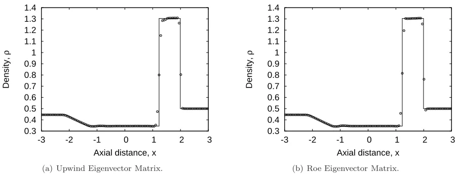
Figure 1. Density at timet= 0.8for the Lax problem, – : analytical solution;◦: numerical solution.

strong contact discontinuity develops which is usually smeared over several cells. The state of the system at t= 0.8 has been computed using 100 cells equally spaced over the domainx∈[−3,3]. The adiabatic index was set toγ= 7/5. Results are shown in Fig.1.

The method is shown to be very accurate with good shock-capturing properties, capturing the shock wave in two points and the contact discontinuity in three points. Modifications of the original method proposed by Tu and Yuan15 _{may be considered, changing the flux splitting technique, the limiter and the characteristic} treatment. We have investigated the effect of such parameters.

The characteristic treatment is the key feature of the method. If the flux is limited component-wise,i.e._,

no projection into characteristic space is performed, spurious low amplitude oscillations appear in velocity and pressure, and a strong overshoot in the density profile appears between the shock and the contact surface. If the characteristic processing is performed, the upwind evaluation of the eigenvector matrices provides a more diffusive scheme, giving a poorer resolution of the contact discontinuity, as is shown in Figure1

The effect of the flux vector splitting technique is not as remarkable. Changing the limiter also has no effect for this test case. In the simulations presented in the rest of the paper, kinetic splitting, Roe average state for the eigenvector matrices and type B limiter were used.

B. Mach 4 Flow past a Cylinder

The supersonic inviscid flow past a cylinder has been simulated. The grid comprises 60×120 cells equally spaced over the domain (r, θ) ∈ [1,4]×[0,2π]. At the far field, non-reflective boundary conditions are enforced, and the free stream primitive variables are:

ρ∞= 7/5, u∞= 4, v∞= 0, p∞= 1,

so that, with γ = 7/5, the free stream speed of sound is a∞ = 1, is solved. Reflective wall boundary conditions are enforced at the surface of the cylinder.

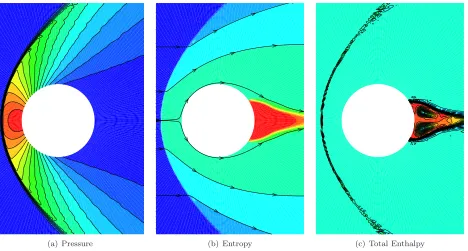
In an inviscid flow the only source of entropy production is the shock wave; as the production of entropy across an oblique shock is a function of the angle between the flow velocity and the shock, it follows that downstream of a bow shock stream lines are entropy isolines. By examining Fig. 2(b), we see that this feature of the ideal solution is predicted.

As the bow shock is adiabatic, the total enthalpy is expected to be constant in the flow field away from the wake. Such a feature is predicted as well, as shown in Figure2(c).

(a) Pressure (b) Entropy (c) Total Enthalpy

C. The Shock Layer

An analytical solution to the Navier-Stokes equations is available for the one-dimensional shock layer prob-lem,19 _{and can be employed as a benchmark for numerical methods. Let subscripts 1 and 2 denote states} upstream and downstream of the shock wave, respectively. As a test case we simulated a steady shock wave, with shock Mach numberMs= 1.5. The upstream conditions are:

ρ1= 7/5, u1= 1.5, p1= 1.

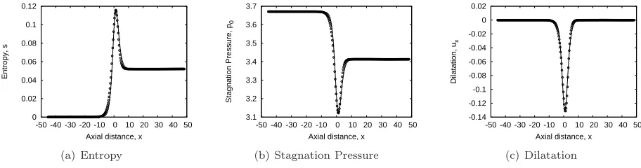
The Prandtl number was set to P r = 3/4 and the isentropic index γ = 7/5. The gas constant was set to R = 5/7, so thatT1= 1, and the downstream conditions are given by the Rankine-Hugoniot relations. A simple linear viscosity law µ=T was assumed. In Fig. 3 the results obtained on 300 linearly spaced cells over the domainx∈[−45,48] are compared to the analytical solution. The challenge for this test case is the correct prediction of dilatation,∂xu, entropy and stagnation pressure. These quantities experience a peak within the shock thickness, which can only be captured if small length scales are well-resolved. As we see from Fig.3there is excellent agreement between the numerical and analytical solutions.

This problem has been simulated using different discretizations, namely CU5-CC6, CU5-CC6-NC and CC5-CC6-K described in Section B. Scheme CU5-CC6-K employs the kinetic splitting for the total flux; for the other two schemes the kinetic splitting for the inviscid flux was employed, so that differences may not be attributed to the splitting techniques. As the results coincide, they are not shown. Hence, we can conclude that, at least for this test case, CU5-CC6-K discretization has proved to be as accurate as the more conventional ones, though less computationally expensive.

0 0.02 0.04 0.06 0.08 0.1 0.12

-50 -40 -30 -20 -10 0 10 20 30 40 50

Entropy, s

Axial distance, x

(a) Entropy

3.1 3.2 3.3 3.4 3.5 3.6 3.7

-50 -40 -30 -20 -10 0 10 20 30 40 50

Stagnation Pressure, p

0

Axial distance, x

(b) Stagnation Pressure

-0.14 -0.12 -0.1 -0.08 -0.06 -0.04 -0.02 0 0.02

-50 -40 -30 -20 -10 0 10 20 30 40 50

Dilatation, u

x

Axial distance, x

(c) Dilatation

Figure 3. Solutions to the shock layer problem, – : analytical solution;◦ : numerical solution.

D. Self-similar Boundary Layer

A laminar boundary layer over a flat plate has also been simulated. The computational domain is (x, y)∈ [−0.1,1.7]×[0,1.2]m2_{. The free stream Mach number, Reynolds number per meter and temperature are} M∞ = 2, Re∞,1 = 2.96×105m−1 and T∞ = 117K, respectively. The boundary conditions are inflow at the left and top boundary, outflow at the right boundary. The bottom boundary is an inflow boundary up to x= 0, and then a no-slip insulated wall. The fluid is air, with isentropic index γ = 7/5, gas constant Rair = 287.06m2/s2K and Prandtl numberP r = 0.725. A grid convergence analysis has been done. The coarser grid is made of 54×135 cells; the grid is equally spaced in thexdirection and refined near the wall in theydirection, with minimum cell size ∆ymin= 5×10−4_{m. In the finer grid the number of cells is double} in both directions. The boundary layer profiles at stationx= 1.4mare compared to the self-similar profiles obtained by the Crocco method20 _{in Fig.4. The nondimensional velocity, temperature and shear stress are} plotted:

u∗=u/u∞, T∗=T /T∞, τ∗=

τx,ypRe∞,x 1/2ρ∞u2∞

,

0 0.1 0.2 0.3 0.4 0.5 0.6 0.7 0.8 0.9 1

0 1 2 3 4 5 6 7 8

Velocity, u

*

Wall distance, y*

(a) Non-dimensional velocity

1 1.1 1.2 1.3 1.4 1.5 1.6 1.7 1.8

0 1 2 3 4 5 6 7 8

Temperature, T

*

Wall distance, y*

(b) Non-dimensional temperature

0 0.1 0.2 0.3 0.4 0.5 0.6 0.7

0 1 2 3 4 5 6 7 8

Shear stress,

τ

*

Wall distance, y*

(c) Non-dimensional shear stress

Figure 4. Boundary layer profiles, – : analytical solution;: numerical solution54×135cells; ◦: numerical solution108×270cells.

E. Blunted Cone

The final test case is hypersonic flow past a blunted cone. The geometry and the conditions are those in the experiment carried out by Cleary et al.21 _{The cone has a 15}◦ _{half-angle, a nose curvature radiusR = 1in}

and a base diameterdb = 12in. The free stream Mach number, Reynolds number per foot and stagnation temperature are:

M∞= 10.6, Re∞,1= 106f t−1, T0= 2000◦R.

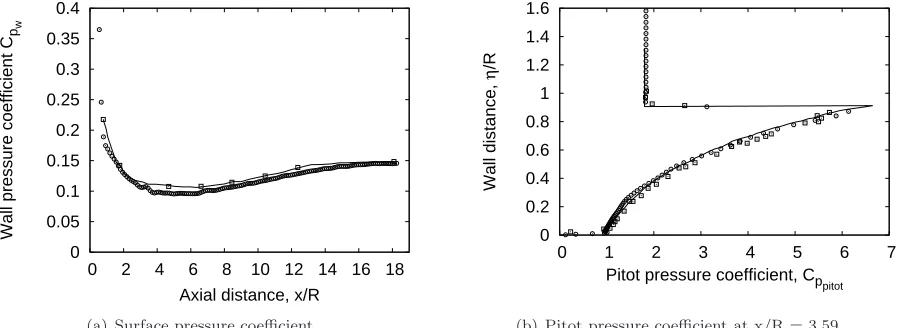
The far field boundary is a parabola, with minimum and maximum distance from the body surfaceηmin= 0.18inandηmax= 3.5in, respectively. The grid is made of 158×78 cells, refined near the wall with minimum cell thickness ∆ηmin = 4×10−4_{in. The cone has no angle of attack, so the axisymmetric formulation has} been used. The boundary conditions are: reflecting wall on the axis, inflow at the far field, outflow at the outlet, no-slip insulated wall at the body surface. The fluid is air, with isentropic indexγ= 7/5, gas constant Rair = 287.06m2/s2K and Prandtl number P r = 0.725. Results are shown in Fig. 5and compared to the experiment and the analytical inviscid solution obtained via the method of characteristics. The pressure coefficient

Cp=

p−p∞ 1/2ρu2

∞

,

is plotted, with pbeing the wall pressure in Fig.5(a), and the Pitot pressure in Fig.5(b). The numerical results have excellent agreement with both the experiment and the analytical solution.

0 0.05 0.1 0.15 0.2 0.25 0.3 0.35 0.4

0 2 4 6 8 10 12 14 16 18

Wall pressure coefficient C

pw

Axial distance, x/R

(a) Surface pressure coefficient

0 0.2 0.4 0.6 0.8 1 1.2 1.4 1.6

0 1 2 3 4 5 6 7

Wall distance,

η

/R

Pitot pressure coefficient, C_p

pitot

(b) Pitot pressure coefficient at x/R = 3.59

V.

Conclusion

A novel scheme for solving the Navier-Stokes equations has been proposed, which is suitable for the simulation of hypersonic flows. The scheme has very high formal accuracy, high resolution properties and is not as computationally demanding as other methods with comparable accuracy. It has been validated against analytical solutions and experimental data and has been shown to be accurate and stable. Future development will involve further validation of the scheme and inclusion of rarefaction effects into the physical model.

References

1

Lele, S. K., “Compact finite difference scheme with spectral-like resolution,”Journal of Computational Physics, Vol. 103, 1992, pp. 16–42.

2

Cook, A. W. and Cabot, W. H., “A high-wavenumber viscosity for high-resolution numerical method,” Journal of Computational Physics, Vol. 195, 2004, pp. 594–601.

3

Cook, A. W. and Cabot, W. H., “Hyperviscosity for shock-turbulence interaction,”Journal of Computational Physics, Vol. 203, 2005, pp. 379–385.

4

Fiorina, B. and Lele, S. K., “A artificial nonlinear diffusivity method for supersonic reacting flows with shocks,”Journal of Computational Physics, Vol. 222, 2007, pp. 246–264.

5

Cook, A. W., “Artificial fluid properties for large eddy simulation of compresible turbulence mixing,”Physics of Fluids, Vol. 19, 2007, pp. 055103.

6

Harten, A., Engquist, B., Osher, S., and Chakravarthy, S., “Uniformly high order essentially non oscillatory schemes, III,”Journal of Computational Physics, Vol. 71, 1995, pp. 231–303.

7

Shu, C. W. and Osher, S., “Efficient implementation of essentially non-oscillatory shock-capturing schemes,”Journal of Computational Physics, Vol. 77, 1988, pp. 439–471.

8

Shu, C. W. and Osher, S., “Efficient implementation of essentially non-oscillatory shock-capturing schemes II,”Journal of Computational Physics, Vol. 89, 1983, pp. 32–78.

9

Pirozzoli, S., “Conservative hybrid compact-WENO schemes for shock-turbulence interaction,”Journal of Computational Physics, Vol. 178, 2001, pp. 81–117.

10

Adams, N. A. and Shariff, K., “A high-resolution hybrid compact-ENO scheme for shock-turbulence interaction problems,”

Journal of Computational Physics, Vol. 127, 1996, pp. 27–51.

11

Ren, Y. X., Liu, M., and Zhang, H., “A characteristic-wise hybrid compact-WENO scheme for solving hyperbolic con-servation lows,”Journal of Computational Physics, Vol. 192, 2003, pp. 365–386.

12

Cockburn, B. and Shu, C. W., “Nonlinearly stable compact schemes for shock calculations,”SIAM Journal of Numerical Analysis, Vol. 31, 1994, pp. 607–627.

13

Yee, H. C., “Explicit and implicit multidimensional high-resolution shock-capturing methods: formulation,”Journal of Computational Physics, Vol. 193, 1997, pp. 216–232.

14

Ravichandran, K. S., “Higher order KFVS algorithms using compact upwind difference operators,”Journal of Compu-tational Physics, Vol. 130, 1997, pp. 161–173.

15

Tu, G. H. and Yuan, X. J., “A characteristic-based shock-capturing scheme for hyperbolic problems,”Journal of Com-putational Physics, Vol. 225, 2007, pp. 2083–2097.

16

Tu, G. H., Yuan, X. J., Xia, Z. Q., and Hu, Z., “A class of compact upwind TVD difference schemes,”Applied Mathematics and Mechanics, Vol. 27, 2006, pp. 765–772.

17

Zhong, X., “High-order finite-difference schemes for numerical simulation of hypersonic boundary layer transition,” Jour-nal of ComputatioJour-nal Physics, Vol. 144, 1998, pp. 662–709.

18

Chou, S. Y. and Baganoff, D., “Kinetic flux-vector splitting for Navier-Stokes equations,” Journal of Computational Physics, Vol. 130, 1997, pp. 217–230.

19

Lagerstrom, P. A.,Laminar flow theory, Princeton University Press, Princeton, 1964.

20

Crocco, L., “Sulla trasmissione del calore da una lamina piana a un fluido scorrente ad alta velocit`a,” L’Aerotecnica, Vol. XII, 1932, pp. 181–197.

21