Global error estimation in CFD mesh coarsening process for uncertainty quantification methods

IAC-13-C2.7.3x18517

GLOBAL ERROR ESTIMATION IN CFD MESH COARSENING PROCESS FOR UNCERTAINTY QUANTIFICATION METHODS

Martin Kubicek

University of Strathclyde, Glasgow, UK, [email protected]

Edmondo Minisci

University of Strathclyde, Glasgow, UK, [email protected]

Due to high performance of modern computers, Uncertainty Quantification is becoming an important part of engi-neering design. Every non intrusive Uncertainty Quantification method requires a considerable number of evaluations of the model, meaning that the design process is more expensive in terms of computational resources/time. In Com-putational Fluid Dynamics, the usual practice is to reduce the comCom-putational time by reducing the number of nodes of the used mesh. Each coarsening of the mesh leads to the increase of the error measured as the difference between the real solution and the solution provided by the computational model. In this work, an approach for quantification of the global error around the stochastic domain, in a mesh reduction process, is described and results obtained for a test case are detailed. The method is based on a comparison of the high accurate mesh against coarse mesh with lower accuracy, but less expensive in terms of computational time. The global error is defined as a volume difference between surrogate models created in the stochastic domain. The stochastic domain is given by pre-specified input variables with appropriate boundaries. Surrogate models are used and a non intrusive polynomial chaos model is cre-ated with response samples from high and low accuracy mesh. For the chosen test case, the input variables, relcre-ated to the stochastic space, were the free stream pressure and free stream Mach number. A hypersonic flow solver developed at the von Karman Institute, Cosmic, was used to compute properties of a flow around the reentry spacecraft. A com-putational expensive mesh was used as a reference mesh. Due to comcom-putational resources, it was impossible to use expansive mesh for Monte Carlo simulation or high order Polynomial Chaos. Therefore, the global error estimation approach was applied to find an accurate and relatively inexpensive mesh for Uncertainty Quantification in hypersonic simulation. Multiple meshes with different coarsening were tested, based on expert knowledge of the problem. The global error estimation method allowed for finding a final mesh, with an error on the mean value 0.48% and on the standard deviation 5.89%, which was 4 times faster than the reference mesh.

I. INTRODUCTION

Uncertainty is one of the key aspects of engineering de-sign, and errors in uncertainty quantification can lead to significant loss in quality or failure in sub-systems, which can lead to catastrophic failure of the whole system. It should be expected that methods for uncertainty quantifi-cation will play a crucial role in future computer aided design. There is a lot of research interest in Uncertainty Quantification (UQ) field and a lot of crucial problems were solved in past, but very little has been done regard-ing the pre-processregard-ing of the problem itself. It is well known that one of the crucial problems in Computational Fluid Dynamics (CFD) is domain discretization [1]. The problem of mesh generation becomes even more severe in case of uncertainty analysis/quantification as combina-tion of multiple inputs over a stochastic space can create non-expected behavior such as in case of chemical

sys-tems [2]. UQ is always associated to a sampling of the system model, which in case of Monte Carlo (MC) ap-proach could require thousands or even more model eval-uations [3]. This stresses the need to reduce as much as possible the computational resources for each evaluation. This highlights the necessity to operate with meshes as coarse as possible and, at the same time, limiting the er-ror introduced by the coarsening of the mesh. This work is focused on a proposed methodology for coarsening of CFD grids during UQ campaigns.

do-main, but the change in the computational domain will modify also the stochastic space. Where the stochastic space is a space created by random variables, represented by probability distributions.

In previous works, focus was on grid coarsening only in physical space, and many books and articles, such as [4, 5, 6] are written about this field. On the other side, only very few articles were published on grid conver-gence in terms of a stochastic space. The interest in coarsening procedures was showed in [7] for an ignition problem involving a single random variable. In [2], the first approach for coarsening techniques was showed, but only in sense of stochastic space. Unfortunately, this ap-proach is not applicable on surrogate non-intrusive tech-niques, because it requires direct modification of the solv-ing code and adjoint solution of given equations. Sensi-tivity analysis done on a grid refinement is described in [8], but sensitivity is used as a guidance to the process of grid coarsening in a physical space and application to a stochastic space is missing. Clearly there is need for a suitable coarsening procedure, especially for problems characterized by a large number of random parameters.

The paper is structured in the following way. First, the iterative approach and its basic idea are described. Then surrogate modeling techniques and sampling strate-gies for surrogate models are described, and the proposed approach is detailed. In the third main section, a numer-ical test case is presented and results are analyzed and commented. A conclusive section summarizes the work and anticipates future activities.

II. THEORY OF ITERATIVE PROCESS OF A GRID COARSENING

Every grid coarsening process is iterative and the basic steps are 1) grid creation, and 2) judgment of a given grid based on predefined criteria. Decision criteria for judg-ment of acceptance/nonacceptance are usually based on multiple aspects such as Richardson error estimation[8]. In the same way, the iterative process of grid coarsen-ing in a stochastic space is iterative too, followcoarsen-ing a loop involving i) grid definition, ii) error estimation, and iii) coarsening of the physical grid. The definition and mod-ification of the grid is based on expert knowledge.

The Iterative Surface (IS) process of a grid coarsen-ing is based on the comparison of grids with different re-finements. Each grid is sampled along a stochastic space and, using these samples, a surrogate model is built for each grid. Then, a hyper-volume is computed under each surrogate model (integration of surrogate model over the stochastic space) and these hyper-volumes are compared. For a proper comparison, a process of normalization on both surrogate models is applied. The normalization as-sures that obtained results are comparable to each other during the iterations and proper judgment can be done on

the result.

The hyper-volume difference is computed via equa-tion (1). The obtained result,, is a value between 0 and 1, where 0 stands for complete agreement and 1 stands for complete disagreement between models. The equa-tion (1) will be a quantitative measurement of a quality of a grid around a stochastic space

= (

Z 1

0 Z 1

0 ...

Z 1

0

|FR(xn1...xnn)−

FT(xn1...xnn)|dxn1dxn2...dxnn)1/n (1)

whereFR stands for the normalized reference surro-gate model,FTstands for the normalized tested surrogate model, andn stands for the number of dimensions, i.e. number of random variables. The subtraction between surrogate models is a way to obtain a hyper-volume be-tween surrogate models. The root of degreen, which is performed after the integration, can be seen as the sup-pression of the effect of different dimensionality. For ex-ample, in case of the same stochastic error between sur-rogate models, but different number of dimensions, the IS equation without then-root would lead to a different result. This is undesirable, because with increasing num-ber of dimensions, the result would approach zero. The integration is performed over the whole stochastic space and boundaries of a stochastic space are given by bound-aries of given random variables. Therefore, the neces-sary number of integrals is exactly equal to the number of dimensions, i.e. random variables, due to the fact that the error between surrogate models has to be quantified around the whole stochastic space. It should be noted that, in most cases, it is necessary to perform numerical integration, since analytic integration is not possible.

The surrogate models are build from samples obtained using different types of grids. Reference surrogate model is build from responses, i.e. quantities of interest, corre-sponding to the reference grid, and tested surrogate mod-els are build from responses corresponding to the tested grid. Both responses are obtained at the same positions in the stochastic space. It is necessary to scale the out-put of both surrogate models in a way that the integration boundaries can be between 0 and 1, as discussed later on in this paper.

III. SURROGATE MODELS

for forward/backward uncertainty quantification method-ology regarding our hyper-sonic problem, the most effi-cient way to propagate uncertainties is to use the Gener-alized Polynomial Chaos expansion (gPC) [10].

The Polynomial Chaos (PC) was first described by Weiner in [11] and it was proven in [12] that it is pos-sible to approximate any well behaved function with PC. The PC was later extended in [13] to different continuous probability distribution types to Generalized Polynomial Chaos, which is derived from the family of hypergeomet-ric orthogonal polynomials known as the Askey scheme. The gPC can be seen as a function decomposition and according to [14] any continue random variable can be represented by an expansion

X= ∞

X

i=1

aiΦ(ξ) (2)

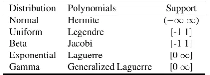
whereΦi(ξ)is a set of orthogonal polynomials from the Askey scheme, ai is the projection ofX on Φi(ξ) andξis an artificial random variable, whose probability density function (PDF) optimally corresponds to the or-thogonal polynomials according to Table 1.

Distribution Polynomials Support

Normal Hermite (−∞ ∞)

Uniform Legendre [-1 1]

Beta Jacobi [-1 1]

Exponential Laguerre [0∞]

Gamma Generalized Laguerre [0∞]

Table 1: Askey scheme of Polynomials

In most cases, polynomials are chosen accordingly to distribution of a given random variable. However, ac-cording to [14], the other polynomials from Table 1 pro-vide valid representation of any given random variable with slightly impaired convergence rate. Therefore, it is legitimate to represent any given continuous random variable with any single polynomial basis. For this work, Legendre polynomial basis was used for all input random variables as the Legendre polynomials represent a uni-form distribution.

The iterative surface approach is a non-intrusive ap-proach. Therefore, it was necessary to use a Non-Intrusive generalized Polynomial Chaos (NIPC). The point collocation NIPC, which is used in this work, was used in work of [15] to solve uncertainty propagation to a selected stochastic CFD cases. Later, the point collo-cation NIPC was extended for an efficient propagation of arbitrarily distributed parametric uncertainties. Briefly, to find ai coefficients required by the equation (2), the well known least square approach was applied. The least squares problem is

a= (ZTZ)−1ZTy (3)

whereyis the corresponding set of simulation output, Zis matrix composed of given polynomials:

Z=



  

Φ1(ξ(1)) Φ2(ξ(1)) ... Φn(ξ(1))

Φ1(ξ(2)) Φ2(ξ(2)) ... Φn(ξ(2)) ... ... ... ...

Φ1(ξ(n)) Φ2(ξ(n)) ... Φn(ξ(n)) 

  

(4)

Full description of NIPC with applications can be seen in [3, 16, 17, 18, 19].

In this work, the first order tensor product PC expan-sion has been adopted for the convergence process. The first order PC expansion is not high enough to capture all uncertainty aspects of the hypersonic flow, but it assured convergence of the iterative process. The third order PC expansion has been adopted for error checking and com-parison of the reference and final grid. The third order is high enough to intercept nonlinear behavior of the given function and to capture peak value of observed responses, i.e. quantity of interest. Also, it is not extremely expen-sive in terms of necessary number of required sampling points.

Design of experiment - definition of collocation points

A lot of different fundamental designs are proposed for NIPC. Since least square approach allows to use ran-domly spread sampling points over the stochastic space, Uniform Design (UD) was selected as Design of Exper-iment (DOE) methodology. The UD was developed by Wang and Fang in 1994 [20], and it was mainly devel-oped for computer based experiments, where a low num-ber of sampling points is allowed. The UD efficiently ex-plores the whole stochastic space by spreading the pling points on the stochastic space, so that the sam-pling points are uniformly distributed in the sense of a low discrepancy [21]. The UD is based on the stochastic representation and the inverse transformation of the MC method.

The creation of UD is not straight forward and requires an optimization process, where the target is to minimize the centered L2-discrepancy. Multiple types of UD exist (see [22] for more details) and, for this work, a design created by minimizing the Centered L2 Discrepancy us-ing Random Samplus-ing was selected. Details about UD and centered L2-discrepancy can be found in [9]. The number of sampling points is based on degree of PC and accordingly to [23], a suggested number of samples used on creation of PC should be 2 times more than minimal number of samples required for the given order of PC.

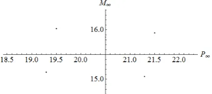
Mach number (M∞). The selection of these two stochas-tic variables is discussed later. For the IS process, the lowest possible number of samples should be used and the necessary minimal number of sampling points for the 1st order NIPC are 4 samples. These 4 samples were spread uniformly around stochastic space and are showed in Figure 1.

Figure 1: Uniform Distribution of sampling points for 1st order NIPC

To obtain accurate statistical properties of the mea-sured response, the 3rd order NIPC was selected. The necessary minimal number of sampling points for the 3rd order NIPC is 10 and accordingly to mention rule, a num-ber of sampling points equal to 20 was selected. The UD is showed in Figure 2.

Figure 2: Uniform Distribution of sampling points for 3rd order NIPC

The selected stochastic distribution for both stochastic variables was the uniform probability distribution, which is represented by the Legendre basis in case of NIPC. The Legendre basis puts an equal weight on each sample in the stochastic space. This helps to properly explore the whole stochastic space and does not emphasize the center of the stochastic space as in case of the Hermite polyno-mials.

IV. NORMALIZATION

The purpose of normalization is to obtain comparable re-sults in each iteration. It is done before integration, so the integration limits can be from 0 to 1, corresponding to the lower and the upper bounds of the stochastic space for each stochastic random variable, respectively. It can

be clearly seen that after normalization, the result of the integration will vary between 0 and 1, which corresponds to percentage difference between the reference surrogate model and tested ones. The normalization of input vari-ables is done by applying equation (5)

xni(xi) = (max(xi)−min(xi))xi+min(xi) (5)

wherexis input of samples for given variable,min(x)

is lower bound of given variable,max(x)is upper bound of given variable. This transformation is done for each random stochastic variable.

One of the very important aspects of iterative surfaces approach is that also surrogate models are normalized, i.e. the quantity of interest obtained from the surrogate model is normalized. Therefore, the output can only vary between 0 and 1. The first step, to normalize the out-put, is to find a minimum and a maximum value in given stochastic space. This is done by using constraint opti-mization method, able to find a global optima on a surro-gate model. This can be written in following way

F Rmin=min

xn FRO(xn) subject to 0≤xn≤1

(6)

F Rmax=max

xn FRO(xn) subject to 0≤xn≤1

(7)

F Tmin=min

xn FT O(xn) subject to 0≤xn≤1

(8)

F Tmax=max

xn FT O(xn) subject to 0≤xn≤1

(9)

where FRO is the non-normalized reference surrogate model, FT O is the non-normalized tested surrogate model andxnare normalized inputs accordingly to equa-tion (5). An Evoluequa-tionary Algorithm (EA) was applied to obtain both optima - maximum and minimum. Algo-rithms for evolutionary optimization and their description can be found in [9]. For this work, a differential evolution algorithm was used. Above obtained values of minimum and maximum were used in following equations to obtain normalization of the response, i.e. the quantity of interest

FR(xn) =

FRO(xn)−min(F Tmin, F Rmin)

max(F Tmax, F Rmax)−min(F Tmin, F Rmin))

FT(xn) =

FT O(xn)−min(F Tmin, F Rmin)

max(F Tmax, F Rmax)−min(F Tmin, F Rmin))

(11)

where FRO is the non-normalized reference surro-gate model,FT Ois the non-normalized tested surrogate model, min(F Tmin, F Rmin) is a smaller value from values F Tmin and F Rmin obtained in equations (8) and (6), max(F Tmax, F Rmax) is a larger value from values F Tmax and F Rmax obtained in equations (9) and (7). These functions (10,11) were used directly in the IS equation (1) to obtain an error between different grids.

The application of normalization of inputs and also, the responses can be seen as scaling functions into the n-dimensional hyper-cube with a length equal to 1, al-ways leading to a hyper-volume equal to 1, independent on number of dimensions. Volume difference between functions, scaled in this hyper-cube, will be then percent-age difference between functions.

V. ITERATION PROCESS - STEP BY STEP

The Iterative Process can be summarized in steps:

1. Create a reference grid for the CFD problem.

2. Create a stochastic space for the CFD problem by selecting random variables and their boundaries.

3. Distribute sample points around the stochastic space using UD. These sample points and their responses, i.e. quantities of interest, will be used to create the non-normalized reference/tested surrogate model.

4. Obtain responses, i.e. quantities of interest, from samples created in step 3 using the reference grid.

5. Create the non-normalized reference surrogate model using NIPC with the Legendre polynomials. The surrogate model will be created using responses from step 4.

6. Normalize the inputs accordingly to the equa-tion (5).

7. Find a maximum and a minimum value, accordingly to equations (6,7), for the non-normalized reference surrogate model by applying an EA.

8. Normalize the non-normalized reference surrogate model accordingly to the equation (10).

9. Manually create/modify the tested coarse grid for the CFD problem. Creation/modification of the grid should be based on the expert knowledge of the given problem.

10. Obtain responses, i.e. quantities of interest, from samples created in step 3 using the coarse grid.

11. Create the non-normalized tested surrogate model using NIPC with the Legendre polynomials. The surrogate model will be created using responses from step 10.

12. Find a maximum and a minimum, accordingly to equations (9,8), for the non-normalized tested sur-rogate model by applying an EA.

13. Normalize the non-normalized tested surrogate model accordingly to the equation (11).

14. Compute the IS equation (1) and obtain a quantifi-cation of the normalized error.

15. Repeat from step 9, until the error between given surrogate models is in acceptable range.

VI. CODE FOR ESTIMATION OF FLOW PROPERTIES AROUND REENTRY CAPSULE

For the continuation of the manned space exploration programme, a more accurate prediction of the heat flux on the spacecraft is required. The designs of Apollo, Galileo, and Huygens are known to be famous examples of lucky heat shield design with barely enough safety fac-tors. A model for hyper-sonic flow around a vehicle was developed in the von Karman Institute (VKI), Cosmic Code. The code was used to design and study the Ther-mal Protection System of a reentry vehicle. It is based on finite volume Navier-Stokes equations with chemical non-equilibrium and thermal equilibrium assumptions. It assumes that the gas can be described as a continuum, meaning that the macroscopic properties can be identi-fied with the average values of the appropriate molecular quantities at any location in the flow. It assumes also, full reversibility of all elementary reactions. Therefore, there is a balance between dissociation and recombination.

used. The amount of particles, which recombine at the wall is given by a probability of recombination. In case of our problem, the recombination probability was set to 0.05 which is equal to 5% of the overall impinging heat flux. At the wall, it was assumed the radiate wall equi-librium to compute the necessary temperature for a re-combination. The radiate wall equilibrium assume that the heat flux released from the gas to the wall is exactly balanced by the heat flux radiated by the wall itself.

The code Cosmic is based on a solution of a mixture of reacting gases, which are modeled as a set of parabolic differential equations with stiff source term. Moreover, the problem is not continues and a strong sonic shock is present. In case of this work, a Hybrid Upwind Splitting (HUS) scheme with fixed shock was used. HUS scheme is combination of van Leer scheme with additional anti-diffusive term. For 2-D axi-symmetrical codes, the infa-mous Carbuncle effect is an issue. The Carbuncle effect is a wrong solution of the heat flux and the pressure at the stagnation point for fully converged solution. It is rep-resented by a peak value of the heat flux/pressure at the stagnation point and by the sonic wave instability. It is not fully understood why the Carbuncle effect is happening and, currently, there is no robust solution to this problem. Therefore, additional dissipation near axis of revolution was added to prevent the Carbuncle effect. This semi-empirical solution prevented the Carbuncle effect in the most cases. For further details about the Carbuncle effect see [24, 25].

Based on the forward analysis made in [26], the largest influence on the stagnation heat flux of the spacecraft had two parameters, the Free Stream Pressure and the Free Stream Mach number. These two parameters were then selected for the grid convergence study. The nominal val-ues for those two parameters are summarized in Table 2 and the other main parameters necessary to perform the simulation are summarized in Table 3.

Random Variable Unit Upper bound

Lower bound Free Stream Pressure [Pa] 18 23 Free Stream Mach

Number

[-] 14.5 16.5

Table 2: Input nominal values

Input conditions Unit Nominal Value

Altitude [Km] 60

Free Stream Tempera-ture

[Kelvin] 245.5

Angle of Attack [Degree] 0

Table 3: Free stream conditions

VII. NUMERICAL APPLICATION OF ITERATIVE SURFACES APPROACH

One of the most important parts in CFD is the conver-gence of the grid and stability of the solution. Not prop-erly defined grid can lead to crash of the final solution in a better case and non-detectable errors in a final solu-tion in the worst case. In case of hyper-sonic flows, the grid needs to take into account shock creation and move-ment of the shock through the physical space. Moreover, in case of 2-D axi-symmetrical problems, such as in this case, the infamous Carbuncle effect appears. The final coarsened grid must be able to avoid all these problems in the whole stochastic space. The reference grid can be seen in Figure 3.

Figure 3: Reference grid at the stagnation point

The target of the UC process is to obtain the Proba-bility Density Function (PDF) of measured quantities, or just their statistical characteristics. For this work, the measured quantity was the heat flux at the stagnation point. The reference grid provides a stable and accurate solution all over the stochastic space. Moreover, it is re-sistant to the Carbuncle effects in the whole stochastic space and proper convergence has been assured all over the stochastic space. Any further refinement of the refer-ence grid did not brought any improvement of the mea-sured quantity. The properties of the reference grid can be found in Table 4, where all simulations were performed on CPU AMD quad 2.5GHz.

Computation time [Min] 122

Grid nodes [-] 21 x 44

Table 4: Properties of the reference grid

sample point forP∞= 27.7andM∞= 15.325can be seen in Figure 4.

Figure 4: Stagnation heat flux at the nose of the space-craft

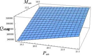
The reference grid provides a reliable solution over the whole stochastic space. Unfortunately, the reference grid is not fast enough to be efficiently used for the UQ cam-paign, when the needed number of samples can be con-siderably high (up to hundreds or thousands for MC ap-proach). The target of the iterative surface process was to obtain a fast grid, which could be later used for MC based or PC based UQ. The required grid had to be re-sistant to the Carbuncle effect over the whole stochastic space. Also, it has to provide a stable and a convergent solution for all possible combinations of input random variables. To check the validity of the coarsening process in the stochastic space, the reference non-normalized sur-rogate model for the reference grid was created using the first order NIPC. The NIPC was created using 4 samples over the stochastic space and observed variable was the heat flux at the stagnation point. Due to the 2-D nature of the problem, it is possible to visualize the problem and therefore, the resulting NIPC surface is showed in Fig-ure 5.

Figure 5: Heat flux function over the stochastic space us-ing the 1st_{order NIPC and the reference grid}

In each iteration, the first order NIPC surface was

cre-ated and compared with the reference NIPC using the IS process. The results of the IS process of grid coarsening are showed in Figure 6

Figure 6: Convergence of the Iterative Surfaces process

where the number of iteration performed until the final coarse grid was obtained is on the X-axis, and the error computed by the equation (1) is showed on the Y-axis.

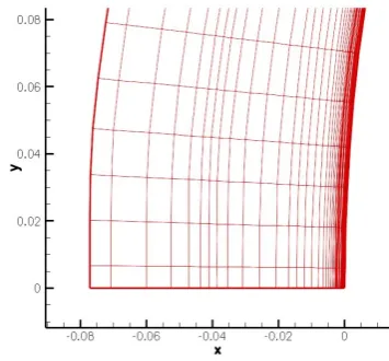
The grid coarsening in the physical space was done manually, based on expert knowledge with aim to provide reliable estimation of the heat flux at the stagnation point. Compared to the reference grid, the coarsening process of the grid was mainly done in area between shock and boundary layer. It was also, found that the solution of the heat flux is not sensitive to very coarse grid around the shock area. The movement of the shock caused by change in stochastic inputs was neither creating any un-predictable behavior. It was found that the Carbuncle effect can occur in certain parts of a stochastic space if the grid is not properly coarsened in the whole stochas-tic space. It is still not clear why the Carbuncle effect appears in some areas of the stochastic space and not in others. The final coarse grid is showed in Figure 7.

The properties of the final coarse grid are summarized in Table 5.

Computation time [Min] 29

Grid [-] 21 x 32

Table 5: Properties of obtained grids

Figure 7: Final coarse grid

Figure 8: Heat flux function over the stochastic space us-ing the 3rdorder NIPC

Stochastic conditions Unit Nominal Value Mean value of the Heat

Flux using the 3rd _order NIPC

[W] 315539

Standard deviation of the Heat Flux using the 3rd or-der NIPC

[W] 29581.1

Mean value of the Heat Flux using the 1st _order NIPC

[W] 291580

Standard deviation of the Heat Flux using the 1st or-der NIPC

[W] 15329.1

Table 6: Quantities of interest for the reference grid

The resulting 1storder NIPC for the reference grid and for the final coarse grid are showed in Figure 9.

To validate our approach, the 3rdorder NIPC was also created for the final coarse grid. Results of the heat flux using the final coarse grid are summarized in Table 7.

Figure 9: Comparison of the 1st_{order NIPC for the} refer-ence grid and for the final coarse grid

Blue:The reference grid Red:The final coarse grid

Stochastic conditions Unit Nominal Value Mean value of the Heat

Flux using the 3rd _order NIPC

[W] 317073

Standard deviation of the Heat Flux using the 3rd or-der NIPC

[W] 27838.3

Mean value of the Heat Flux using the 1st _order NIPC

[W] 287894

Standard deviation of the Heat Flux using the 1st or-der NIPC

[W] 19843

Table 7: Quantities of interest for the final coarse grid

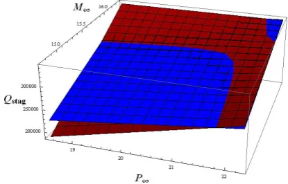
Visualization of the difference between the 3rd _order NIPC for the reference grid and the final coarse grid is showed in Figure 10.

Figure 10: Comparison of the 3rd_{order NIPC for the} ref-erence grid and for the final coarse grid

To compute an error between mean value and standard deviation of given grids, following equations are used

mean =

M eanRef−M eanF in M eanRef (12) std=

StdRef−StdF in StdRef (13)

whereM eanRef is the mean value of the stagnation heat flux obtained using the reference grid,M eanF inis the mean value of the stagnation heat flux obtained us-ing the final coarse grid,StdRefis the standard deviation of the stagnation heat flux obtained using the reference grid, andStdF inis the standard deviation of the stagna-tion heat flux obtained using the final coarse grid. The obtained errors between given grids are summarized in Table 8.

Error of the mean value us-ing the 1st_{order NIPC}

[%] 1.3

Error of the Standard de-viation using the 1st _order NIPC

[%] 29.4

Error of the mean value us-ing the 3rdorder NIPC

[%] 0.48

Error of the Standard de-viation using the 3rd order NIPC

[%] 5.89

Table 8: Normalized error for the mean value and the standard deviation

VIII. DISCUSSION

Results from the IS process show that improvement of computational time can be obtained with very little loss of accuracy (in terms of the mean value and the standard deviation). The IS equation was able to quantify the error between two surrogate models obtained by using differ-ent types of grids. Also, using the IS equation leads to a better understanding of the grid coarsening process in a stochastic sense than just blind coarsening of the grid. It leads to a better understanding of the physical phenom-ena happening in the whole stochastic space.

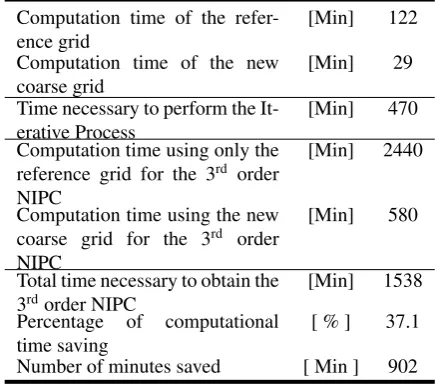
The grid coarsening was done due to necessity to per-form a large number of simulations on expensive CFD problem for UQ. For this work, the IS process was per-formed on a low order NIPC and to prove the conver-gence of the IS process in stochastic sense, the third or-der NIPC was created for both grids and compared. To estimate time saving, the time necessary to build the high order NIPC using the reference grid is compared to the time required to build the the high order NIPC using the coarse grid plus the time required to perform the IS pro-cess. The whole process of obtaining the final coarse grid

took about 470 minutes, considering only the computa-tional time. The time necessary to obtain the 3rd _order NIPC using the reference grid is around 2440 minutes, while the time necessary to obtain the 3rdorder NIPC us-ing the final coarse grid is 580 minutes. Times estimation are summarized in Table 9.

Computation time of the refer-ence grid

[Min] 122

Computation time of the new coarse grid

[Min] 29

Time necessary to perform the It-erative Process

[Min] 470

Computation time using only the reference grid for the 3rd _order NIPC

[Min] 2440

Computation time using the new coarse grid for the 3rd order NIPC

[Min] 580

Total time necessary to obtain the 3rdorder NIPC

[Min] 1538

Percentage of computational time saving

[ % ] 37.1

Number of minutes saved [ Min ] 902

Table 9: Times summarization

Saving of time, in this case, is about 902 minutes, con-sidering only computational time. This means that the process is about 37% faster than using the original grid. It can be concluded that the IS process considerably im-proved time necessary to obtain the high order NIPC.

It is well known, that CFD problems are highly sen-sitive to gradients in a physical space and these gradi-ents can significantly change around the stochastic space. Therefore, only blind grid coarsening over the stochastic space, without any exploration, could lead to a critical er-ror. One very important observation was made: the coars-ening of the grid in only one point can lead to a significant error in uncertainty quantification results. To explain this phenomena, let us examine the first iteration of the itera-tive process, where the error obtained by the IS equation was 94.9%. More precisely, let us have a look at one spe-cific point in the stochastic space. The input conditions for this specific point are summarized in Table 10.

Input conditions Unit Nominal Value The Free Stream Pressure [Pa] 21.7 The Free Stream Mach

Number

[-] 15.325

Table 10: Initial conditions for selected case

the heat flux obtained using the reference grid at this point, the obtained error was estimated to be only 5.47%. This error could be acceptable for this work and this grid showed to be very promising as a time required to com-pute this grid was only 15 minutes. To explain the prob-lem in the stochastic space, let us examine the plot of the heat flux at the stagnation point. The 1storder NIPC us-ing the reference grid and the 1st order NIPC using the grid from the 1st_{iteration are showed in Figure 11.}

Figure 11: Heat flux functions over the stochastic space using the 1storder NIPC

Blue:The reference grid

Red:Grid obtained in the 1st_iteration

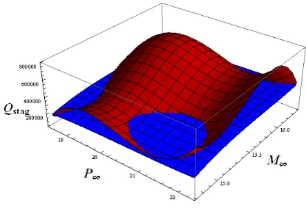
It can be clearly seen that the function does not have the same shape as the function obtained by the reference grid and results from the 1st_{iteration are in complete} dis-agreement with results from the reference grid. Also, the 3rd_{order NIPC is build to compare statistical properties} of given grid in more robust way. The mean value and the standard deviation for the grid from 1st _{iteration are} summarized in Table 11. The comparison of the 3rd_order NIPC surfaces is showed in Figure 12.

It can be clearly seen that using only one sample point in a sense of stochastic space is not recommended, be-cause it can very easily lead to wrong results. The IS equation very easily showed that the grid obtained in the first iteration does not perform well in the sense of uncer-tainty quantification.

IX. CONCLUSION AND FUTURE WORK

The proposed error estimation approach for a grid coars-ening was proved to be working and efficient. The new coarse grid used for Hyper-sonic flows is reliable in a whole stochastic space and the grid is resistant to all as-pects of Hyper-sonic flow such as the Carbuncle effect. The reduction of accuracy was minimal and compared with gain in speed, negligible.

Very important observation about grid coarsening in a stochastic space was made. Coarsening the grid in only one sample point in sense of the stochastic space can lead

Stochastic conditions Unit Nominal Value Mean value of the Heat

Flux using the 1st _order NIPC

[W] 253210

Standard deviation of the Heat Flux using the 1st or-der NIPC

[W] 552627

Mean value of the Heat Flux using the 3rd _order NIPC

[W] 446611.6

Standard deviation of the Heat Flux using the 3rd or-der NIPC

[W] 150887

Error of the mean value us-ing the 1st_{order NIPC}

[%] 53.2

Error of the Standard de-viation using the 1st order NIPC

[%] 903.8

Error of the mean value us-ing the 3rd_{order NIPC}

[%] 41.9

Error of the Standard de-viation using the 3rd _order NIPC

[%] 410.1

Table 11: Quantities of interest for the grid from the 1st iteration

Figure 12: Heat flux functions over the stochastic space. Blue:The reference grid

Red:Grid obtained in the 1st_iteration

to critically wrong results. Therefore, it is suggested, in the worst case, to obtain more than one sample from the stochastic space and, in the best case, perform the itera-tive surface process to obtain reliable and accurate grid.

REFERENCES

[1] A. Bakker.Applied Computational Fluid Dynam-ics - Lecture 7: meshing. 2002. URL: http : / / www . bakker . org / dartmouth06 /

engs150/07-mesh.pdf.

[2] L. Mathelin and O. P. Le Maitre. “Uncertainty quantification in a chemical system using error es-timate based mesh adaption”. In:Theoretical and Computational Fluid Dynamics(2012).

[3] K. Togawa, A. Benigni, and A. Monti. “Advan-tages and Challenges of Non intrusive Polynomial Chaos Theory”. In:Proceedings of the 2011 Grand Challenges on Modeling and Simulation Confer-ence. Society for Modeling and Simulation Inter-national. Vista, CA, June 2011, pp. 30–35.

[4] M. A. Olshanskii. Lecture notes on multigrid methods. English. 2012.URL:www . math . uh . edu / ˜molshan/ftp/pub/lect_notes. pdf.

[5] Z.-y. Shu, G.-z. Wang, and C.-s. Dong. “Adap-tive triangular mesh coarsening with centroidal Voronoi tessellations”. In: Journal of Zhejiang University10.4 (2009), pp. 535–545.

[6] J. F. Shepherd et al. “Adaptive Mesh Coarsen-ing for Quadrilateral and Hexahedral Meshes”. In:

Finite Elements in Analysis and Design 46.1-2 (2010), pp. 17–32.

[7] H. N. Najm et al. “Uncertainty quantification in chemical systems”. In: International journal for numerical methods in engineering80.6 (Dec. 2009), pp. 789–814.

[8] M. S. M. Ali, C. J. Doolan, and V. Wheatley. “Grid convergence study for a two-dimensional simulation of flow around a square cylinder at a low reynolds number”. In: Seventh International Conference on CFD in the Minerals and Process Industries. CSIRO. Melbourne, Australia, Dec. 2009.

[9] K. T. Fang, R. Li, and A. Sudjianto.Design and Modeling for Computer Experiments. New York: Chapman and Hall/CRC press, 2006.

[10] H. Cheng and A. Sandu. “Efficient Uncertainty Quantification with the Polynomial Chaos Method for Stiff Systems”. In:Mathematics and Comput-ers in Simulation 79.11 (July 2009), pp. 3278– 3295.

[11] N. Wiener. “The homogeneous chaos”. In: Amer-ica Journal of Mathematics 60.4 (Oct. 1938), pp. 897–936.

[12] R. H. Cameron and W. T. Martin. “The orthogonal development of nonlinear functionals in series of Fourier Hermite functionals”. In:Annals of Math-ematic48.2 (Apr. 1947), pp. 385–392.

[13] R. A. Askey and J. A. Wilson. “Some Basic Hy-pergeometric Polynomials that Generalize Jacobi Polynomials”. In:American Mathematical Society,

319 (1985).

[14] D. Xiu. “Fast Numerical Methods for Stochastic Computations: A Review”. In:Communications in computational physics5.2-4 (Feb. 2009), pp. 242– 272.

[15] S. Hosder, R. Walters, and R. Perez. “A Non-Intrusive Polynomial Chaos Method For Uncer-tainty Propagation in CFD Simulations”. In:44th AIAA Aerospace Sciences Meeting and Exhibit. Reno, Nevada, Jan. 2006.

[16] M. Eldred and J. Burkardt. “Comparison of Non-Intrusive Polynomial Chaos and Stochastic Col-location Methods for Uncertainty Quantification”. In:47thAIAA Aerospace Sciences Meeting includ-ing The New Horizons Forum and Aerospace Ex-position. American Institute of Aeronautics and Astronautics. Orlando, Florida, Jan. 2009.

[17] H. Cheng and A. Sandu. “Collocation Least-squares Polynomial Chaos Method”. In:

SpringSim ’10, Proceedings of the 2010 Spring Simulation Multiconference. Society for Computer Simulation International. San Diego, CA, 2010.

[18] D. Xiu and G. E. Karniadakis. “The Wiener– Askey Polynomial Chaos for Stochastic Differ-ential Equations”. In:SIAM Journal on Scientific Computing24.2 (2002), pp. 619–644.

[19] M. S. Eldred et al.DAKOTA, A Multilevel Parallel Object-Oriented Framework for Design Optimiza-tion, Parameter EstimaOptimiza-tion, Uncertainty Quantifi-cation, and Sensitivity Analysis: Version 5.0 User’s Manual. Tech. rep. SANDIA national laboratories, Feb. 2013.

[20] K. T. Fang and Y. Wang.Number-Theoretic Meth-ods in Statistics. London: Chapman and Hall, 1994.

[21] K. T. Fang and Y. Wang.Number-theoretic Meth-ods in Statistics. London: Chapman and Hall, 1994.

[22] K.-T. Fang et al. Uniform Design Tables. Mar. 2000.URL: http : / / uic . edu . hk / isci /

[23] S. Hosder, R. W. Walters, and M. Balch. “Ef-ficient Sampling for Non-Intrusive Polynomial Chaos Applications with Multiple Uncertain Input Variables”. In:48th _{AIAA/ASME/ASCE/AHS/ASC} Structures, Structural Dynamics, and Materials Conference. Honolulu, HI, Apr. 2007.

[24] R. W. MacCormack. “The Carbuncle CFD Prob-lem”. In:49th AIAA Aerospace Sciences Meeting including the New Horizons Forum and Aerospace Exposition. Orlando, Florida, Jan. 2011.

[25] J.-C. Robinet et al. “Shock wave instability and the carbuncle phenomenon: same intrinsic origin?” In:

Journal of Fluid Mechanics417 (2000), pp. 237– 263.