Using CAViaR models with implied volatility for value-at-risk estimation

Using CAViaR Models with Implied Volatility

for Value at Risk Estimation

Jooyoung Jeon*

Smith School of Enterprise and the Environment, University of Oxford

James W. Taylor

Saïd Business School, University of Oxford

Journal of Forecasting, forthcoming

*

Address for Correspondence:

Jooyoung Jeon

Smith School of Enterprise and the Environment University of Oxford

Hayes House, 75 George Street Oxford OX1 2BQ, UK

Tel: +44 (0)1865 288927 Fax: +44 (0)1865 288805

Using CAViaR Models with Implied Volatility for Value at Risk Estimation

Abstract

This paper proposes VaR estimation methods that are a synthesis of conditional autoregressive value at risk (CAViaR) time series models and implied volatility. The appeal of this proposal is that it merges information from the historical time series and the different information supplied by the market’s expectation of risk. Forecast combining methods, with

weights estimated using quantile regression, are considered. We also investigate plugging implied volatility into the CAViaR models, a procedure that has not been considered in the VaR area so far. Results for daily index returns indicate that the newly proposed methods are comparable or superior to individual methods, such as the standard CAViaR models and quantiles constructed from implied volatility and the empirical distribution of standardised residual. We find that the implied volatility has more explanatory power as the focus moves further out into the left tail of the conditional distribution of S&P500 daily returns.

JEL classification: C22, C53, G17

1. Introduction

Value at risk (VaR) has become a standard tool for measuring market risk. It involves the estimation of the maximum potential loss of the market value of an asset or a portfolio over a certain time horizon at a given confidence level, which is typically chosen to be 1% or 5%. Thus, estimating the VaR involves forecasting tail quantiles of the conditional distribution of returns. The accurate assessment of the exposure to market risk of a financial institution is of great importance for internal risk control. Despite its conceptual simplicity and popularity as an industrial standard, no consensus has been reached as to the best method for estimating VaR.

The conditional autoregressive value at risk (CAViaR) models of Engle and Manganelli (2004) provide an appealing approach to VaR estimation. These models avoid distributional assumptions by modelling the quantile directly using quantile regression. They are autoregressive in structure, which is intuitively attractive, as series of financial returns tend to exhibit volatility clustering. A variety of alternative time series modelling approaches have been presented, including the use of GARCH volatility models, extreme value theory and exponentially weighted quantile regression (see Manganelli and Engle, 2004; Kuester et al., 2006; Taylor, 2008b). Empirical evidence has shown that CAViaR models are competitive with other VaR models (Bao et al., 2006; Yu et al., 2010). An approach that contrasts with these time series methods is to base VaR estimation on the implied volatility, which is the expectation of volatility implied by the options market (see Chong, 2004; Christoffersen and Mazzotta, 2005; Giot, 2005). This approach constructs quantile forecasts using the implied volatility and a distributional assumption.

supplied by two or more separate forecasting methods in order to improve forecasting accuracy (Bunn, 1989). However, the focus in the literature has largely been on the combination of point forecasts. Although a number of studies have investigated the combination of volatility forecasts, there are very few papers on the combination of quantile forecasts. This is perhaps a little surprising, as it is now more than twenty years since Granger (1989) and Granger et al. (1989) originally proposed combining quantile forecasts. In this paper, we consider similar combining methods to those proposed by Granger et al. However, in contrast to their application to monthly economic time series, our focus is VaR estimation for daily financial returns data, and we use different individual quantile forecasting methods. In addition to the combining methods, we also evaluate the worth of including, in a CAViaR model, an additional regressor that is a quantile predictor based on implied volatility. We are not aware of any other studies that have considered the synthesis of CAViaR and implied volatility for VaR estimation.

In Section 2, we briefly review the literature on VaR estimation. Section 3 discusses the use of implied volatility for the prediction of volatility and VaR. In Section 4, we describe our approaches to combining VaR estimates. Section 5 presents CAViaR models that include, as an extra regressor, a quantile estimator based on implied volatility. Section 6 is an empirical study in which we evaluate the proposed approaches to combining VaR forecasts for daily stock index returns. The final section summarises the paper and provides concluding comments.

2. Value at Risk

example is a GARCH volatility model with a Student-t distribution or perhaps an asymmetric t distribution (see, for example, Mittnik and Paolella, 2000). A notable benefit of a parametric method is the complete formation of the conditional returns distribution. A significant pitfall of a parametric approach is that the specification of the variance equation and the choice of distribution may be wrong.

The most widely used nonparametric method is historical simulation. With this method, the VaR is estimated as the quantile of the empirical distribution of historical returns from a moving window of the most recent periods. The advantage of historical simulation is that it requires no distributional assumption and that it is easy to compute. However, the VaR estimation can be poor and slow to converge to the actual VaR, especially for the extreme quantiles. Another difficulty, recognised by Boudoukh et al. (1998), is in the choice of the number of observations to include in the moving window. A moving window that is too small leads to large sampling errors, while too many observations in the moving window results in sluggish adaptation to the dynamic changes in the true distribution. Boudoukh et al. (1998), Mittnik and Paolella (2000) and Taylor (2008b) attempt to overcome this issue through their exponentially weighted approaches to VaR estimation.

The semiparametric VaR category includes applications of extreme value analysis and methods based on quantile regression, such as the CAViaR models introduced by Engle and Manganelli (2004). Using an autoregressive framework, CAViaR models aim to derive the evolution of the desired quantile rather than extracting the quantile from an estimate of a complete distribution or from a volatility estimate. The approach has the advantage of allowing the shape of the conditional returns distribution to be time-varying, and for the time-variation to be different for different quantiles of the distribution. The four CAViaR models introduced by Engle and Manganelli (2004) and the AR(1)-GARCH(1,1) CAViaR model proposed by Kuester et al. (2006) are presented in the following expressions:

1 3 1

2 1 ( )

)

(   t  t

t Q y

Q     

Asymmetric Slope CAViaR:

) 0 ( ) 0 ( ) ( )

(  ₁₂Q_1 ₃y_1 I  ₄y_1 I 

Q_{t t t t}

Indirect GARCH(1,1) CAViaR:













1 2 1 3 2 1 2 1 ( )

5 . 0 2 1 )

(     t  t

t I Q y

Q      

Indirect AR(1)-GARCH(1,1) CAViaR:













1 2 2 1 3 2 2 1 2 1 1

4 1 2 0.5 ( ( ) ) ( )

)

(  t     t  t  t  t

t y I Q y y y

Q         

Adaptive CAViaR:

















1 1 1

1( ) 1 exp ( )

)

(  t      t  t  

t Q G y Q

Q

where Qt() is the  quantile conditional upon t-1, the information set up to time t-1; I is an

indicator function which returns a value of one if the argument is true, and zero otherwise; G

is some sizeable positive number; and the i are parameters. Note that we are modelling here a

residual term, yt, defined as yt=rt–E(rt|t-1), where rt is the return and E(rt|t-1) is the

conditional expectation, which is often assumed to be zero or a constant. The parameters are determined by the quantile regression (Koenker and Bassett, 1978) minimisation, which is of the following form:





t t t t|yt Qt t t

Q y Q

y ( ) 1 ( )

min (1)

used for the GARCH volatility model. The indirect AR(1)-GARCH(1,1) CAViaR model allows for the conditional mean to be time-varying. The second term in the adaptive CAViaR model is a function that forces the quantile to take a lower value if yt falls below the quantile, and a higher value otherwise. As G, the function converges to the hit variable, defined as





 t t

t I y Q

H    . Engle and Manganelli (2004) note that the structure of the adaptive

CAViaR model is such that the estimator learns nothing from the extent to which the quantile

has or has not been exceeded since it considers only whether Qt() is larger than yt or not.

3. Using Implied Volatility for Predicting Volatility and VaR

3.1. Implied Volatility

Implied volatility represents the volatility of the underlying security that is implicit in the market price of an option according to a particular model. In other words, the implied volatility is the level of volatility in the Black-Scholes formula that delivers an option price equal to the current market price. In contrast to historical volatility, which is a measure of price changes in the past, implied volatility reflects the market’s expectations regarding future volatility. There has been a growing trend towards the use of implied volatility as a key variable in financial investment decisions, risk management, derivative pricing, market making, market timing and portfolio selection.

In this paper, we do not use implied volatility for volatility estimation, but instead we use it for VaR estimation. We consider the benefit of combining quantile forecasts based on implied volatility and CAViaR time series models. Before we present this idea in more detail, let us first briefly review the related literature.

3.2. Comparison and Synthesis of Volatility Forecasting Approaches

predictions from time series models. Although many studies conclude in favour of implied volatility, others find no significant benefit in using implied volatility over predictions from a time series model.

Looking at the relatively recent literature, we find that Szakmary et al. (2003) conclude that implied volatility outperforms historical volatility as a predictor of the realised volatility in a large majority of 35 futures markets including equity indices, interest rates, currencies, commodities and crude oil. Pong et al. (2004) find historical intraday returns have significant incremental information in exchange rates, beyond the implied volatility information, for horizons up to one week, while for longer horizons, implied volatility provides more informative forecasts than historical volatility. Corredor and Santamaria (2004) report that implied volatility clearly dominates all of the time series models such as the GARCH family. Giot and Laurent (2007) find that implied volatility delivers more relevant volatility information content than historical volatility for stock indices such as the S&P100 and S&P500. However, there is also recent evidence suggesting that there is value in both implied volatility and volatility based on the historical time series of returns, and that the superiority of each depends on the financial time series considered and the time series method used. Noh and Kim (2006) conclude that both implied volatility and historical volatility using high-frequency returns can outperform each other in forecasting volatility. In their empirical test, historical volatility from high frequency returns performed better in the FTSE100 futures, which tends to be relatively close to normally distributed, while the result of implied volatility was better in the S&P500 futures, which displays excess skewness even with volatilities from high frequency returns.

weights in a linear combination of individual forecasts. In contrast to the literature on combining forecasts of the level, research into combining volatility forecasts is far less well developed (Poon and Granger, 2003). Of the studies that do exist, there is general support for the idea of forming a linear combination of historical volatility and implied volatility (see Kroner et al., 1995; Doidge and Wei, 1998; Pong et al., 2004). It is also worth noting that there is evidence in favour of combining volatility forecasts constructed from the same information set, such as two GARCH models (see, for example, Amendola and Storti, 2007).

An approach that is related to combining forecasts is to include implied volatility as an exogenous variable in the time series model, such as a GARCH model. In general, this ‘plug-in’ approach has been performed with the emphasis on testing for an improvement in

in-sample fit (e.g. Day and Lewis, 1992; Blair et al., 2001). However, some authors have also evaluated the resulting forecasts using post-sample data (e.g. Claessen and Mittnik, 2002; Giot, 2005; Donaldson and Kamstra, 2005).

3.3. Forecasting VaR using Implied Volatility

implied volatility, historical volatility and volatilities from GARCH models. They find that implied volatility provides the most accurate volatility forecasts for all currency exchange rates and forecast horizons considered. Yet, in the application of the volatility forecasts to density estimation, they conclude that the density and interval forecasts based on implied volatility do not capture the tail behaviour of the distribution. However, the assumption of Gaussian tail shape might be a weakness in the studies of Chong (2004) and Christoffersen and Mazzotta (2005). In this paper, we make no distributional assumptions in our investigation of the usefulness of implied volatility for quantile estimation.

3.4. Combining VaR Forecasts from Time Series Models and Implied Volatility

If there is support for forecasting quantiles using implied volatility and also evidence in favour of time series methods for quantile prediction, there is some appeal in producing a quantile forecast from the combination of one quantile forecast based on implied volatility and another constructed from historical returns. There are very few studies that have looked at the combination of quantile forecasts. Granger (1989) and Granger et al. (1989) introduce the idea of using quantile regression to combine quantile forecasts. Granger et al. (1989) apply the idea to quantile forecasts produced using time series methods for two monthly economic time series. Using simulated data, Taylor and Bunn (1998) assess the usefulness of different restrictions on the parameters of the quantile regression combination. Giacomini and Komunjer (2005) describe how encompassing tests can be performed for two quantile predictors using the quantile regression combining framework. They apply their proposal to the S&P500 VaR estimates based on two time series volatility forecasting methods.

volatility, we are not aware of any studies that have directly estimated VaR using a combination of quantile predictions based on implied volatility with forecasts from a time series model. Our proposal is to do just this. We consider combinations of two attractive individual VaR approaches, namely the CAViaR models and a simple VaR estimator based on implied volatility, which we call the implied quantile (IQ) and present in Section 3.5. We describe the different combining methods in Section 4.

3.5. Implied Quantile (IQ)

We construct an implied quantile (IQ) estimator for period t as the product of implied

volatility recorded in the previous period, implied t1

 , and the quantile, Emp()

Q , of an empirical

distribution, which we construct as the distribution of the in-sample values of yt, defined in Section 2, standardised by implied volatility. The IQ estimator can be expressed in the following form:

implied

t Emp IQ

t Q

Q () () 1 (2)

In basing quantile estimation on implied volatility, the IQ approach captures the market’s expectation of future risk. Another advantage is that the method does not assume a

particular distribution for the asset returns, and it involves no parameter estimation. We also considered the use of a Gaussian assumption, but the post-sample forecasting results were comfortably superior for the empirical distribution. It is interesting to note that this simple approach to capturing an ‘implied quantile’ assumes returns standardised with implied

4. Combining Implied Quantile and CAViaR

4.1. Simple Average Combining (SimpAvg)

The simplest and most widely used forecast combining method is to take the simple arithmetic mean of the individual forecasts. We consider the simple average of the quantile forecasts from the IQ method and one CAViaR model, as in expression (3). When presenting our empirical results, we refer to this method as ‘SimpAvg’ combining.

( ) ( ) 2 ( )

1 2

1  

 CAViaR

t IQ

t

t Q Q

Q   (3)

4.2. Unrestricted Linear Combination (LinearComb)

A traditional approach to combining is to compute linear combinations of forecasts. Granger et al. (1989) apply this combining method to quantile forecasts using quantile regression to optimise the parameters. We also use this method to combine the CAViaR and IQ forecasts. The resultant quantile forecast is of the following form:

) ( )

( )

( ₁ ₂  ₃ CAViaR

t IQ

t

t Q Q

Q    , (4)

where the i are parameters estimated using the quantile regression minimisation of

expression (1). As expression (4) is linear, the minimisation can be performed efficiently using linear programming (see Koenker and Bassett, 1978). We refer to this method as ‘LinearComb’.

4.3. Weighted Averaged Combining (WtdAvg)

forecasts are biased, arguing that gains in efficiency can be made at the cost of some bias. Bunn (1989) strengthens the case for a weighted average combination by explaining that it can be more robust than an unconstrained model. With these benefits in mind, we included in our study the weighted average of the individual forecasts from the CAViaR models and the IQ. The resultant quantile forecast is of the following form:

()  ()





CAViaR t IQ

t

t Q Q

Q    , (5)

where  is a combining weight constrained to be between zero and one, which is estimated using quantile regression. As with the ‘LinearComb’ method, linear programming can be

used to optimise the combining parameter. We refer to this method as ‘WtdAvg’ combining. As Taylor and Bunn (1998) point out, one benefit of the weighted average method, as in expression (5) above, is that the value of the weight, , indicates the relative explanatory

powers of the two quantile predictors.

4.4. Weighted Average Combining Optimised using Exponential Weighting (WtdAvgExp)

This method is similar to the weighted average combination method of Section 4.3, but different in that it uses exponentially weighted quantile regression (EWQR) (see Taylor, 2008b) for the optimisation of the combining weight . The intuition of the EWQR method is that it gives more weight to more recent observations in the quantile regression optimisation. Boudoukh et al. (1998) assert that, as series of financial returns exhibit time-varying and cyclical volatility, an exponential weighting approach presents a reasonable trade-off between statistical precision and adaptiveness to recent news. The EWQR minimization has the following form:





t t|y_t Q_t t t

t T t t t T Q y Q

y ( ) 1 ( )

min ,

where Qt()is a weighted average combination of the form of expression (5). A lower value

to the recent observations and less historical information is captured. In Section 6, we

describe how we optimised the value of  in our empirical study. In the discussion of our empirical results, we refer to this method as ‘WtdAvgExp’.

5. Plugging the Implied Quantile into CAViaR (PlugIn)

In Section 3.2, we discussed how implied volatility has been merged with GARCH models by simply plugging the implied volatility into the statistical models as an additional regressor. In this section, we present the analogous idea for quantile estimation, which involves the IQ predictor being plugged into the CAViaR models from Section 2. The resultant ‘PlugIn’ CAViaR models are presented in expressions (6) to (10).

Symmetric Absolute Value PlugIn:

) ( )

( )

( 1 2 1 3 1   IQ t IQ t t

t Q y Q

Q       (6)

Asymmetric Slope PlugIn:

() ₁ _{2 1}() _{3 1} ( ₁ 0) _{4 1} ( ₁ 0)  IQ()

t IQ t t t t t

t Q y I y y I y Q

Q   _  _{ }   _{ }   (7)

Indirect GARCH(1,1) PlugIn:













1 2 2 1 3 2 1 2

1 ( ) ( )

5 . 0 2 1 )

(    _t   _t _{IQ t}IQ 

t I Q y Q

Q     _  _ 

(8) AR(1)-GARCH(1,1) PlugIn:













1 2 2 2 1 3 2 2 1 2 1

1 1 2 0.5 ( ( ) ) ( ) ( )

)

(  t    t   t  t  t IQ tIQ 

t y I Q y y y Q

Q  _     _  _  _  _ 

(9) Adaptive PlugIn:

( ) ( )

















1 1 1 3 1 2

1       

  IQ t IQ t t t

t Q G y Q Q

Q            (10)

These models enable an understanding of the importance of implied volatility by inspecting the coefficient, IQ, of the implied quantile predictor for different  quantiles.

(1), which is used to optimise the standard CAViaR models. We are not aware of any previous research that has considered the ‘CAViaR PlugIn’ models presented in this section.

6. Empirical Study

In this section, we compare the accuracy of the VaR estimation from the methods presented in Sections 4 and 5 with that of the standard CAViaR models and the IQ estimator. Our study used daily log returns for the S&P500 and the DAX30 stock indices, and their respective implied volatility indices, the VIX and the VDAX. The VIX is derived from S&P500 index call and put options of a wide range of strike prices that are further weighted to represent a hypothetical at-the-money option with a constant maturity of 22 trading days (30 calendar days) to expiry. The VDAX is constructed by call and put DAX index options of eight different strike prices that are further linearly interpolated to a remaining life of 45

Period 1 and its volatile post-sample period as Post-sample 1. The later sample is referred to as Period 2, and its relatively tranquil post-sample period is referred to as Post-sample 2. We report the results for both samples, which enables us to check the consistency of our results under challenging and stable market conditions.

--- Figures 1 and 2 ---

For both indices, we subtracted from each return, rt, the mean, , of the 2,500

in-sample returns. The quantile estimation methods were applied to the resulting residuals, yt =

rt - . The confidence level of VaR is typically chosen to be 1% or 5%. Our study evaluates

forecast accuracy for the 1%, 5%, 95%, and 99% conditional quantiles. For a trader who is long in the index, the left quantile (e.g. 1% and 5%) is relevant because the trading losses occur on the left side of the returns density. However, for a trader who is short in the index, the right quantile (e.g. 95% and 99%) is more relevant because trading losses occur on the right side of the returns density.

6.1. Implementation of the VaR Estimation Methods

found that the indirect AR-GARCH CAViaR model outperformed the simpler indirect GARCH CAViaR model.

To optimise the standard and IQ PlugIn CAViaR models of Sections 2 and 5, linear programming cannot be used to perform the quantile regression minimisation due to the nonlinearity of the problem. Instead, we performed the optimisation using both the approach proposed by Engle and Manganelli (2004) in their published paper and the approach that they used in the 1999 draft of the paper. The 1999 version of the paper used the differential evolutionary genetic algorithm by Storn and Price (1997), while the published version used a quasi-Newton optimisation algorithm. Our optimisation proceeded by first generating 105 vectors of parameters from a uniform random number generator between 0 and 1, or between -1 and 0, depending on the appropriate sign of the parameter. For each of the vectors, the quantile regression summation (QRSum) of expression (1) is evaluated. Then two approaches were used for further optimisation. In the first, the 10 vectors that produced the lowest values for the QRSum out of the 105 vectors of parameters were used as the best initial values in a quasi-Newton optimisation routine. In the second approach, the 200 vectors that produce the lowest values for the QRSum 105 vectors of parameters are used as the population in the genetic algorithm, which involved 2,000 generations and, following Engle and Manganelli, a mutation parameter of 0.8 and crossover parameter of 0.5. Out of the two further optimisation methods performed, the vector producing the lowest QRSum was chosen as the final parameter vector. In this study, all the computations were performed in Matlab 7.5.0.

To optimise the parameters of the LinearComb and WtdAvg combining methods, we expressed the quantile regression minimisation as a linear programme and applied the Nelder-Mead Simplex algorithm. We used a similar approach for the WtdAvgExp combining

method after first optimising the EWQR decay parameter . To do this, we considered a grid

optimal value of  was chosen as the value that led to the lowest QRSum calculated for the

last 500 observations of the in-sample data. We performed the optimisation separately for

each value of (i.e. for each different quantile).

6.2. In-sample Results for the WtdAvg Combining Method

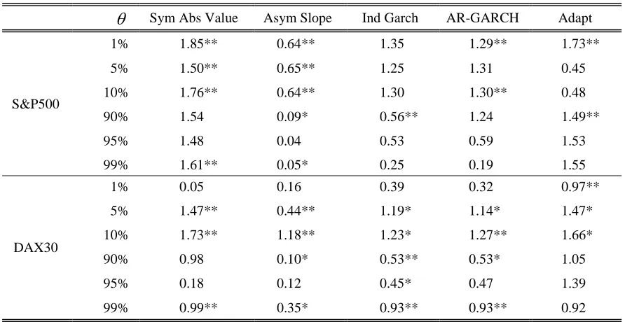
In this section, we report the in-sample estimated values of the weight parameter  in the WtdAvg combining method of expression (5) in Section 4.3. (For conciseness, we restrict attention here to the WtdAvg method, rather than consider the weights in each of the combining methods.) The value of the weight is constrained to lie between zero and one, and thus expresses the explanatory power of the IQ method in relation to the CAViaR model. As described in Section 4.3, the weight is estimated by quantile regression. Table 1 examines how the parameter changes for a range of different values of  for the S&P500 and DAX30 series, respectively. Although the focus of our quantile forecasting empirical study in Section 6.3 is estimation of the 1%, 5%, 95% and 99% quantiles, we also consider in this section the 10% and 90% quantiles. Due to the large overlap between the in-sample data of Periods 1 and 2, the estimated weights were quite similar for the two periods. In view of this, we present only the in-sample results for the more recent set of data, Period 2.

--- Table 1 ---

than by the autoregressive quantile model estimated by quantile regression. There is no such pattern evident in Table 1 for the DAX30. In fact, for the most extreme quantiles that we consider (the 1% and 99% quantiles), the IQ method has a smaller weighting in the lower tail than in the upper tail of the distribution.

A statistical test could perhaps be performed for the combining weight to test whether it is significantly different from zero or from one. However, the standard error and distribution for the test is not straightforward because the weight is constrained to fall between zero and one. Encompassing tests could be used for the LinearComb approach, but implementing such a test is not straightforward in the weighted average case due to the bounds on the value of the weight. This is presumably one reason for why it is not standard practice in the combining literature to carry out tests of the combining weight.

6.3. In-sample Results for the PlugIn Method

Similarly to Section 6.2, we also investigated the in-sample estimated values of the coefficient IQ in the PlugIn method of expressions (6) to (10) in Section 5. Using the

approach of Engle and Manganelli (2004), we performed significance tests of the coefficients.

In Table 2, we present estimated values of the coefficient IQ, along with the results of the

significance test of the hypothesis IQ=0. Table 2 shows that, for approximately half of the

cases, the coefficient IQ is significantly different from zero. This indicates that, for these

values of , implied volatility tends to have incremental information in the PlugIn method. --- Table 2 ---

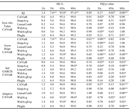
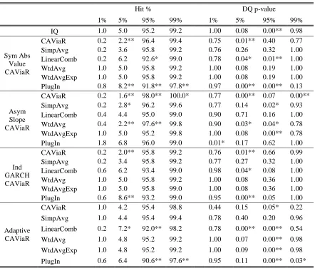
6.4. Post-sample Forecasting Results

Engle and Manganelli (2004). The hit percentage assesses the percentage of observations

falling below the VaR estimator. The ideal value is for estimation of the  quantile. We examined significant difference from this ideal using a test based on the binomial distribution. The Engle and Manganelli DQ test for conditional coverage evaluates whether the dynamic

sequence of the hit variable is distributed i.i.d. Bernoulli with probability , and is

independent of the conditional quantile estimator, Qt() . This test uses a regression

framework to test whether the variable Ht, defined in Section 2, has zero unconditional and conditional expectations. As in the empirical studies of Engle and Manganelli (2004) and Huang et al. (2010), we included four lags of the variable Ht in the test’s regression to deliver a DQ test statistic, which, under the null hypothesis of perfect conditional coverage, is

distributed 2

with six degrees of freedom.

--- Tables 3 to 5 ---

We have four post-sample periods in our study. In Tables 3 and 4, for the S&P500, we present the results for Post-sample 1 and Post-sample 2, respectively. In each table, for each  quantile, we report the hit percentage and the p-value of the DQ test statistic. Table 5 summarises the results of Tables 3 and 4 by presenting the number of occurrences of significance for each method applied to each of the two post-sample periods. Smaller values in Table 5 are better. Table 5 also presents a summary of the corresponding results for the DAX30. To help explain Table 5, let us focus on the first seven rows of values in the table. These seven rows summarise Table 3. In these rows, for each  quantile and each method,

the value shown is the number of entries in Table 3 that were significant at the 5% level for the hit percentage and for the DQ test. Let us consider the interpretation of a value of 1 for the SimpAvg method in the hit percentage column corresponding to the =99% quantile for

considered in Table 3, the hit percentage for the SimpAvg method was significant at the 5% level. The final seven rows of the table average the values in the rows above.

Using Table 5, let us briefly compare the results for the two different post sample periods, Post-samples 1 and 2. For the S&P500, the CAViaR method adapted better to the challenging trading conditions in Post-sample 1 than the IQ method, whereas the IQ method performed better than the CAViaR method in Post-sample 2. For the DAX30, it is not clear which individual method performed better. However, regardless of whether the data series is the S&P500 or the DAX30, or whether the post-sample period is volatile or tranquil, the results for the combining method would seem to be competitive with those of the two individual methods. Turning to the PlugIn method, the results show that it performed reasonably well in Post-sample 1, but it was less competitive for Post-sample 2.

Looking at the average of the hit percentage results in the bottom seven rows of Table 5, it is impressive to see that all the combining methods and the PlugIn method either match or outperform the individual CAViaR and IQ methods for each of the four quantiles. In the fifth column of values, we can see that the average values for the combining methods are better than those for the IQ method and the individual CAViaR methods. Of the seven methods, the LinearComb method produced the best hit percentage results, followed by the SimpAvg and WtdAvgExp combining methods.

and the IQ method. Of the combining methods, the results for the LinearComb and SimpAvg methods are the best.

To summarise, in terms of both the hit percentage and DQ test, the results of the combining methods were better than the two individual methods. The PlugIn method was better than the two individual methods in terms of the hit percentage, but less convincing in terms of the DQ test. Among the combining methods, our study suggests that the LinearComb and SimpAvg methods are the best. As for the reason why the LinearComb method performs better than the WtdAvg method, we would suggest that it may be because the inclusion of the intercept term in the model, and the lack of restrictions on the values of the weights, allows the individual quantile estimators to be debiased. This has certainly been the main argument in favour of the LinearComb method in the context of forecasting the level (or mean) of a time series (see Granger and Ramanathan, 1984). It is worth noting that the WtdAvgExp offered slight improvement over the simpler WtdAvg method in terms of the hit percentage, suggesting that there may be benefit in trying to optimise the combining weight by giving more weight to the more recent observations.

7. Summary and Concluding Comments

the DAX30. Our post-sample forecasting results show that an unrestricted linear combination has the potential to outperform the individual methods. We also obtained encouraging results for the simple average and exponentially weighted average combining methods. Considering the relative scarcity of research on combining methods for estimating VaR, it is hoped that this study will motivate further combining research in this field.

References

Amendola A, Storti G. 2008. A GMM procedure for combining volatility forecasts. Computational Statistics and Data Analysis 52 : 3047-3060.

Bao Y, Lee T-, Saltoglu B. 2006. Evaluating predictive performance of value-at-risk models in emerging markets: A reality check. Journal of Forecasting25 : 101-128.

Barone-Adesi G, Bourgoin F, Giannopoulos K. 1998. Don’t look back. Risk 11 : 100-104. Bates JM, Granger CWJ. 1969. The combination of forecasts. Operations Research

Quarterly 20 : 451-468.

Blair BJ, Poon SH, Taylor SJ. 2001. Forecasting S&P 100 volatility: The incremental information content of implied volatilities and high-frequency index returns. Journal of Econometrics 105 : 5-26.

Boudoukh J, Richardson M, Whitelaw RF. 1998. The best of both worlds. Risk 11 : 64-67. Bunn DW. 1989. Forecasting with more than one model. Journal of Forecasting 8 : 161-166. Chong J. 2004. Value at risk from econometric models and implied from currency options.

Journal of Forecasting 23 : 603-620.

Christoffersen PF, Mazzotta S. 2005. The accuracy of density forecasts from foreign exchange options. Journal of Financial Econometrics 3 : 578-605.

Claessen H, Mittnik S. 2002. Forecasting stock market volatility and the informational efficiency of the DAX-index options market. The European Journal of Finance 8 : 302-321.

Corredor P, Santamaría R. 2004. Forecasting volatility in the spanish option market. Applied Financial Economics 14 : 1-11.

Day TE, Lewis CM. 1992. Stock market volatility and the information content of stock index options. Journal of Econometrics 52 : 267-287.

Doidge C, Wei JZ. 1998. Volatility forecasting and the efficiency of the toronto 35 index options market. Canadian Journal of Administrative Sciences 15 : 28–38.

Donaldson RG, Kamstra MJ. 2005. Volatility forecasts, trading volume, and the ARCH versus option-implied volatility trade-off. The Journal of Financial Research 28 : 519-538. Engle RF, Manganelli S. 2004. CAViaR: Conditional autoregressive value at risk by

regression quantiles. Journal of Business and Economic Statistics 22 : 367-382.

Giacomini R, Komunjer I. 2005. Evaluation and combination of conditional quantile forecasts. Journal of Business and Economic Statistics 23 : 416-431.

Giot P. 2005. Implied volatility indexes and daily value at risk models. Journal of Derivatives 12 : 54-64.

Giot P, Laurent S. 2007. The information content of implied volatility in light of the jump/continuous decomposition of realized volatility. Journal of Futures Markets 27 : 337-359.

Granger CWJ. 1989. Invited review: Combining forecasts–20 years later. Journal of Forecasting 8 : 167-173.

Granger CWJ, Ramanathan R. 1984. Improved methods of combining forecasts. Journal of Forecasting 3 : 197-204.

Granger CWJ, White H, Kamstra MJ. 1989. Interval forecasting: An analysis based upon ARCH-quantile estimators. Journal of Econometrics 40 : 87-96.

Huang D, Yu B, Lu Z, Fabozzi FJ, Focardi S, Fukushima M. 2010. Index-Exciting CAViaR: A New Empirical Time-Varying Risk Model. Studies in Nonlinear Dynamics and Econometrics 14 : art. no. 1.

Koenker R, Bassett G. 1978. Regression quantiles. Econometrica 46 : 33-50.

Kuester K, Mittnik S, Paolella MS. 2006. Value-at-risk prediction: A comparison of alternative strategies. Journal of Financial Econometrics 4 : 53-89.

Manganelli S, Engle RF. 2004. A Comparison of Value-at-Risk Models in Finance. Szegö G. ed. Risk measures for the 21st century. Wiley & Sons: Chichester, UK; 123-143.

Mittnik S, Paolella MS. 2000. Conditional density and value-at-risk prediction of Asian currency exchange rates. Journal of Forecasting 19 : 313-333.

Noh J, Kim TH. 2006. Forecasting volatility of futures market: The S&P 500 and FTSE 100 futures using high frequency returns and implied volatility. Applied Economics 38 : 395-413.

Pong S, Shackleton MB, Taylor SJ, Xu X. 2004. Forecasting currency volatility: A comparison of implied volatilities and AR (FI) MA models. Journal of Banking and Finance 28 : 2541-2563.

Poon SH, Granger CWJ. 2003. Forecasting volatility in financial markets: A review. Journal of Economic Literature 41 : 478-539.

Storn R, Price K. 1997. Differential Evolution–A simple and efficient heuristic for global optimization over continuous spaces. Journal of Global Optimization 11 : 341-359. Szakmary A, Ors E, Kim JK, Davidson III WN. 2003. The predictive power of implied

volatility: Evidence from 35 futures markets. Journal of Banking and Finance 27 : 2151-2175.

Taylor JW. 2008a. Estimating value at risk and expected shortfall using expectiles. Journal of Financial Econometrics 6 : 231-252.

Taylor JW. 2008b. Using exponentially weighted quantile regression to estimate value at risk and expected shortfall. Journal of Financial Econometrics 6 : 382-406.

Taylor JW, Bunn DW. 1998. Combining forecast quantiles using quantile regression: Investigating the derived weights, estimator bias and imposing constraints. Journal of Applied Statistics 25 : 193-206.

Taylor SJ, Xu X. 1997. The incremental volatility information in one million foreign exchange quotations. Journal of Empirical Finance 4 : 317-340.

Yu PLH, Li WK, Jin S. 2010. On Some Models for Value-At-Risk. Econometric Reviews

Table 1 For the in-sample data of Period 2 of the S&P500 and the DAX30, the

WtdAvg combining weight on the IQ method for different values of .

Bold indicates combining weight larger for the IQ method.

 Sym Abs Value Asym Slope Ind Garch AR-GARCH Adapt

S&P500

1% 1.00 0.80 1.00 0.88 1.00

5% 0.99 0.36 0.99 0.75 0.79

10% 0.94 0.40 0.93 0.63 0.54

90% 0.75 0.27 0.54 0.49 1.00

95% 0.64 0.27 0.46 0.52 1.00

99% 0.37 0.09 0.21 0.29 1.00

DAX30

1% 0.50 0.41 0.43 0.34 1.00

5% 0.85 0.43 0.84 0.66 0.99

10% 0.85 0.42 0.78 0.50 0.66

90% 0.73 0.35 0.74 0.57 1.00

95% 0.52 0.33 0.57 0.35 1.00

99% 0.79 0.74 0.73 0.78 1.00

Table 2 For the in-sample data of Period 2 of the S&P500 and the DAX30, the

PlugIn coefficient, IQ, of the IQ estimator for different values of .

 Sym Abs Value Asym Slope Ind Garch AR-GARCH Adapt

S&P500

1% 1.85** 0.64** 1.35 1.29** 1.73** 5% 1.50** 0.65** 1.25 1.31 0.45 10% 1.76** 0.64** 1.30 1.30** 0.48 90% 1.54 0.09* 0.56** 1.24 1.49** 95% 1.48 0.04 0.53 0.59 1.53 99% 1.61** 0.05* 0.25 0.19 1.55

DAX30

1% 0.05 0.16 0.39 0.32 0.97** 5% 1.47** 0.44** 1.19* 1.14* 1.47* 10% 1.73** 1.18** 1.23* 1.27** 1.66* 90% 0.98 0.10* 0.53** 0.53* 1.05 95% 0.18 0.12 0.45* 0.47 1.39 99% 0.99** 0.35* 0.93** 0.93** 0.92

Table 3 Hit percentage and DQ test p-values for Post-sample 1 (volatile) of the S&P500.

Hit % DQ p-value

1% 5% 95% 99% 1% 5% 95% 99%

IQ 1.4 7.6** 93.0* 97.4** 0.85 0.17 0.02* 0.00** Sym Abs

Value CAViaR

CAViaR 0.4 4.4 95.4 99.0 0.91 0.02* 0.78 0.98 SimpAvg 0.4 5.6 95.0 98.6 0.92 0.06 0.31 0.03* LinearComb 0.2 4.4 94.6 99.4 0.78 0.87 0.59 0.98 WtdAvg 0.4 5.6 94.2 98.8 0.90 0.05* 0.43 0.99 WtdAvgExp 0.6 5.6 94.2 99.0 0.99 0.05* 0.43 1.00 PlugIn 1.0 6.4 94.4 99.2 0.93 0.21 0.71 0.97

Asym Slope CAViaR

CAViaR 1.8 7.6** 95.4 99.4 0.01** 0.00** 0.82 0.96 SimpAvg 1.2 6.6 94.0 99.0 0.71 0.00** 0.43 1.00 LinearComb 1.2 5.2 94.8 99.4 0.75 0.23 0.78 0.96 WtdAvg 1.2 6.6 94.8 99.4 0.74 0.00** 0.78 0.96 WtdAvgExp 1.2 6.6 93.0* 98.4 0.65 0.00** 0.01* 0.00** PlugIn 1.8 6.4 95.2 99.6 0.08 0.02* 0.68 0.90 Ind

GARCH CAViaR

CAViaR 0.6 4.4 94.6 98.6 0.74 0.03* 0.23 0.03* SimpAvg 0.8 5.4 94.6 98.0* 0.76 0.04* 0.18 0.00** LinearComb 1.2 4.0 95.4 99.2 0.93 0.83 0.76 1.00 WtdAvg 1.4 5.8 94.6 98.6 0.85 0.06 0.19 0.03* WtdAvgExp 1.4 6.0 94.6 98.6 0.83 0.07 0.20 0.03* PlugIn 1.2 6.4 93.8 98.8 0.98 0.16 0.20 1.00

Adaptive CAViaR

CAViaR 1.2 4.8 94.8 98.8 0.95 0.57 0.13 0.01** SimpAvg 1.2 5.2 93.8 99.0 0.98 0.36 0.08 0.00** LinearComb 1.0 6.2 94.0 99.2 1.00 0.60 0.13 0.00** WtdAvg 1.4 6.0 93.0* 98.0* 0.85 0.78 0.02* 0.01* WtdAvgExp 1.4 6.0 93.0* 98.4 0.85 0.78 0.02* 0.02* PlugIn 1.2 6.4 94.4 99.0 0.98 0.53 0.70 0.00**

Table 4 Hit percentage and DQ test p-values for Post-sample 2 (tranquil) of the S&P500.

Hit % DQ p-value

1% 5% 95% 99% 1% 5% 95% 99%

IQ 1.0 5.0 95.2 99.2 1.00 0.08 0.00** 0.98 Sym Abs

Value CAViaR

CAViaR 0.2 2.2** 96.4 99.4 0.75 0.01** 0.40 0.77 SimpAvg 0.2 3.6 95.8 99.2 0.76 0.26 0.32 1.00 LinearComb 0.2 6.2 92.6* 99.0 0.78 0.04* 0.01** 1.00 WtdAvg 1.0 5.0 95.8 99.2 1.00 0.08 0.19 1.00 WtdAvgExp 1.0 5.0 95.8 99.2 1.00 0.08 0.19 1.00 PlugIn 0.8 8.2** 91.8** 97.8** 0.97 0.00** 0.00** 0.13

Asym Slope CAViaR

CAViaR 0.2 1.6** 98.0** 100.0* 0.77 0.00** 0.07 0.00** SimpAvg 0.2 2.8* 96.2 99.6 0.77 0.14 0.02* 0.93 LinearComb 0.4 4.4 95.0 99.0 0.90 0.71 0.16 1.00 WtdAvg 0.4 2.2** 97.6** 99.8 0.90 0.03* 0.04* 0.78 WtdAvgExp 1.0 5.0 95.2 99.8 1.00 0.08 0.00** 0.78 PlugIn 1.8 6.8 96.0 99.0 0.01* 0.17 0.62 1.00 Ind

GARCH CAViaR

CAViaR 0.2 2.0** 95.8 99.2 0.76 0.01** 0.66 0.99 SimpAvg 0.2 3.4 95.8 99.2 0.77 0.27 0.32 1.00 LinearComb 0.6 6.2 93.4 99.0 0.98 0.04* 0.08 1.00 WtdAvg 1.0 5.0 95.8 99.2 1.00 0.08 0.36 1.00 WtdAvgExp 1.0 5.0 95.8 99.0 1.00 0.08 0.36 1.00 PlugIn 0.6 8.6** 93.2 99.0 0.95 0.00** 0.05 1.00

Adaptive CAViaR

CAViaR 1.0 4.2 95.4 98.8 0.44 0.15 0.05* 0.22 SimpAvg 1.0 4.4 95.4 99.4 0.78 0.40 0.20 0.96 LinearComb 0.2 7.2* 92.0** 98.2 0.78 0.00** 0.00** 0.54 WtdAvg 1.0 4.8 95.2 99.2 1.00 0.07 0.00** 0.98 WtdAvgExp 1.0 4.8 95.2 99.2 1.00 0.09 0.00** 0.98 PlugIn 0.6 6.4 90.6** 97.6** 0.95 0.11 0.00** 0.03*

Table 5 Summary of results for each quantile. For each post-sample period and each method, the value shown is the number of CAViaR models for which the test null hypothesis was rejected. Smaller values are better. In the final seven rows, bold indicates the best performing method in each column.

Hit(%) DQ p-value

1% 5% 95% 99% Mean 1% 5% 95% 99% Mean

S&P500 Post-sample 1

(volatile) (Summary of

Table 3)

IQ 0 4 4 4 3 0 0 4 4 2

CAViaR 0 1 0 0 0.25 1 3 0 2 1.5

SimpAvg 0 0 0 1 0.25 0 2 0 3 1.25

LinearComb 0 0 0 0 0 0 0 0 1 0.25

WtdAvg 0 0 1 1 0.5 0 2 1 2 1.25

WtdAvgExp 0 0 2 0 0.5 0 2 2 3 1.75

PlugIn 0 0 0 0 0 0 1 0 1 0.5

S&P500 Post-sample 2

(tranquil) (Summary of

Table 4)

IQ 0 0 0 0 0 0 0 4 0 1

CAViaR 0 3 1 1 1.25 0 3 1 1 1.25

SimpAvg 0 1 0 0 0.25 0 0 1 0 0.25

LinearComb 0 1 2 0 0.75 0 3 2 0 1.25

WtdAvg 0 1 1 0 0.5 0 1 2 0 0.75

WtdAvgExp 0 0 0 0 0 0 0 2 0 0.5

PlugIn 0 2 2 2 1.5 1 2 2 1 1.5

DAX30 Post-sample 1

(volatile)

IQ 0 4 0 0 1 4 4 0 4 3

CAViaR 0 2 3 1 1.5 1 3 0 1 1.25

SimpAvg 0 3 0 1 1 2 0 0 2 1

LinearComb 0 1 1 0 0.5 1 1 0 0 0.5

WtdAvg 0 4 0 1 1.25 2 1 0 2 1.25

WtdAvgExp 0 4 0 0 1 2 1 0 1 1

PlugIn 0 0 1 0 0.25 2 3 1 2 2

DAX30 Post-sample 2

(tranquil)

IQ 0 0 0 0 0 4 0 0 0 1

CAViaR 0 1 0 0 0.25 3 0 0 0 0.75

SimpAvg 0 0 0 0 0 4 0 0 0 1

LinearComb 0 0 0 0 0 2 0 0 3 1.25

WtdAvg 0 0 0 0 0 4 0 0 0 1

WtdAvgExp 0 0 0 0 0 4 0 0 0 1

PlugIn 0 0 0 0 0 4 0 0 4 2

Mean

IQ 0 2 1 1 1 2 1 2 2 1.75

CAViaR 0 1.75 1 0.5 0.81 1.25 2.25 0.25 1 1.19

SimpAvg 0 1 0 0.5 0.38 1.5 0.5 0.25 1.25 0.88

LinearComb 0 0.5 0.75 0 0.31 0.75 1 0.5 1 0.81

WtdAvg 0 1.25 0.5 0.5 0.56 1.5 1 0.75 1 1.06

WtdAvgExp 0 1 0.5 0 0.38 1.5 0.75 1 1 1.06