PEA: Polymorphic Encryption Algorithm based on quantum computation

City, University of London Institutional Repository

Citation

:

Communications, 3(1), pp. 1-18. doi: 10.1504/IJSCC.2011.039222

This is the unspecified version of the paper.

This version of the publication may differ from the final published

version.

Permanent repository link: http://openaccess.city.ac.uk/2509/

Link to published version

:

Copyright and reuse:

City Research Online aims to make research

outputs of City, University of London available to a wider audience.

Copyright and Moral Rights remain with the author(s) and/or copyright

holders. URLs from City Research Online may be freely distributed and

linked to.

City Research Online: http://openaccess.city.ac.uk/ [email protected]

PEA: Polymorphic Encryption Algorithm

Based on Quantum Computation

Nikos Komninos and Georgios Mantas

Algorithms and Security Group

Athens Information Technology

GR-19002 Peania Attiki, Greece

[email protected]

Abstract

In this paper, a polymorphic encryption algorithm (PEA), based on basic quantum computations, is

proposed for the encryption of binary bits. PEA is a symmetric key encryption algorithm that

applies different combinations of quantum gates to encrypt binary bits. PEA is also polymorphic

since the states of the shared secret key control the different combinations of the ciphertext. It is

shown that PEA achieves perfect secrecy and is resilient to eavesdropping and Trojan horse

attacks. A security analysis of PEA is also described.

Keywords. Encryption algorithm, polymorphism, quantum computations, CNOT

and SWAP quantum gates.

1. Introduction

Conventional cryptography consists of two types of cryptosystems; symmetric

key cryptosystems and asymmetric key, or public key cryptosystems. Symmetric

key cryptosystems, as the name implies, use identical keys for encryption and

decryption and both the sender and the receiver share the same key(s). For this

reason, such cryptosystems rely on the secrecy of the key. Otherwise, any

malicious actors can deduce the plaintext from the ciphertext. The major

disadvantage of such cryptosystems is the need of frequent and reliable key

distribution. On the contrary, cryptosystems based on asymmetric key

cryptography use different keys for ciphering and for deciphering. In ciphering,

the key is announced publicly, but in deciphering, the key remains secret. The

generation is based on computational complexity of certain difficult mathematical

problems. However, the main drawback of this cryptosystem is the computational

cost of generating the key pair [19, 20].

In the early 1970s, a new type of Cryptography was proposed by Stephen

Wiesner [10]. He proposed the idea of Quantum Cryptography as he introduced

the concept of quantum conjugate coding at the same year. Quantum

Cryptography is based on quantum computation. In contrast to Conventional

Cryptography that uses digital bits for encoding information, Quantum

Cryptography uses quantum particles (i.e. photons) and their quantized properties

(i.e. photon’s polarization) to do that. Each photon carries one bit of quantum

information, called qubit. A qubit defines not only the two binary eigenstates "0"

and "1" but also the superposition of the two. Furthermore, the security of

Quantum Cryptography is based on fundamental quantum mechanical principles.

It uses the quantum mechanics in order to overcome the key distribution problem

which is the most serious problem in the both types of conventional cryptography

[6, 8, 9 10, 18]. Quantum Cryptography is considered as the basis for next

generation cryptographic systems that may be able to replace the public key

cryptosystems [3, 4, 7, 11, 16].

Conventional cryptosystems are susceptible to advanced technology, as

new more powerful computers (e.g. quantum computers) may be able to override

the burden of computationally complex problems in the future. Thus, no matter

how strong a cryptographic algorithm is, soon or later it will be broken. On the

contrary, Quantum Cryptography is independent of technological advance in the

future as its security is provable information theoretically [4, 5].

During the last two decades, the Quantum Cryptography has focused on three

fields concerned to key sharing between transmitter and receiver. These fields are

the following: quantum key distribution [8], quantum secret sharing [10] and

quantum bit commitment [1]. Furthermore, a new breakthrough appeared

regarding the evolution of quantum encryption algorithms. The concept of this

new field was first introduced by Boykin and Roychowdhury [12] in 2000. Thus,

Quantum Cryptography does not only provide a secure key exchange between two

parties, but also provides a special type of quantum encryption at transmitter and

Moreover, Quantum Cryptography solves the two major practical

problems of one-time pad encryption scheme as it provides secure key distribution

and is also able to generate sets of random numbers at the two communicating

parties,. One – time pad is the only provably unconditionally secure cryptosystem,

which can not be compromised even in the face of unlimited time and

computational power [17, 19, 20]. Therefore, the existing encryption algorithms

for quantum information take the form of one-time pad encryption method.

Several quantum encryption algorithms for classical binary bits from different

aspects were proposed in [2, 13, 14]. A realizable quantum encryption algorithm

for qubits was also presented in [15]. Motivated by these and the challenge of

quantum computing field, we propose a polymorphic encryption algorithm (PEA),

which uses different combinations of quantum CNOT and SWAP gates in order to

encrypt messages without changing the key. The Controlled NOT gate (CNOT) is

the quantum analogue of the XOR gate. It has two input qubits, the first is the

controlled qubit and the second is the target qubit. If the controlled qubit is zero

then the target qubit is intact. If the controlled qubit is one then the target qubit is

flipped. Generally, the notation CNOTx,y, means that the index x is the controlled

qubit and the index y is the target qubit. The quantum SWAP gate has two input

qubits and swaps them. The notation SWAPx,y, means that this gate swaps the

qubit x with the qubit y. The security of the encryption algorithm is analyzed from

several aspects and it is shown that the PEA can prevent quantum and classical

attack.

Following this introduction, the paper is organized as follows. Section 2

describes the polymorphic encryption algorithm along with its encryption and

decryption processes. Section 3, presents a security analysis of PEA and shows

how resilient is to quantum and classical attacks. Finally, we conclude our

algorithm in section 4 and propose future work.

2. Polymorphic Encryption Algorithm

The polymorphic encryption algorithm (PEA) is a symmetric key algorithm based

on quantum computation for encryption of classical messages. PEA requires four

groups of keys to be exchanged between sender and recipient before the

quantum ancilla bits. The second group key is responsible for the choice of the

first level of encryption. The third group key is responsible for the second level of

encryption and finally, the fourth group key is responsible for leading the

encrypted data to non-orthogonality. Hence, the pre-sharing of these keys is

essential as they are used during encryption of PEA. The polymorphism of this

algorithm is based on the pre-shared keys, as they are the factors that designate

the internal paths that the algorithm should follow in order to give the encrypted

output.

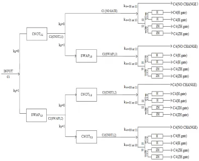
Figure 1. PEA Encryption Algorithm

Generally, the classical message, which is encrypted by PEA, consists of m bits

and for each bit of the message one quantum state, C1, is created based on the

current bit and the key. So, m quantum states are going to be created. As

illustrated in figure 1, the input of PEA is C1, which according to the second group

of key element k2 can follow one of the two paths. If k2 is equal to 0, the quantum

state will go through CNOT2,1 gate. Whereas k2 is equal to 1, the quantum state

will pass either by the path which has no gate or by the SWAP1,3, according to the

third group key element k3. Likewise, the output of SWAP1,2 gate, C2(SWAP1,2),

will pass either by CNOT1,2 gate or by CNOT3,2, according to the third group key

element k3.

2.1. Encryption

The encryption process consists of the following phases: preparation; first and

second level of encryption; and non-orthogonality phases.

Phase 1: Preparation

In Phase 1, the key k1 is used for the definition of the valid quantum states. Let we

define the quantum ancilla state represented as | 12 1 1k

k _{〉. The} k11_{and the} 2 1

k _{are two}

key elements of the ith key pair in k1. When the classical key element pairs are 00,

01, 10 and 11 we have the corresponding quantum ancilla states |00〉, |01〉, |10〉, | 11〉, respectively. For each bit, m (0 or 1), of the classical message, we have the corresponding quantum state |m〉. Now, the combination of the quantum ancilla state with the corresponding quantum state |m〉 of each bit, will give all valid quantum states. This combination is achieved by using the tensor product which

generates the tensor product state | 12 1 1k

mk 〉. To simplify our calculations, we have assumed an 8-bit classical message as a block size for our algorithm. Thus, we are

going to have the following eight valid quantum states:

|000〉, |001〉, |010〉, |011〉, |100〉, |101〉, |110〉, |111〉.

These valid states can be represented by Equation 1:

} 1 , 0 { , , ,

| ₁1 ₁2 ₁1 ₁2 1 = mk k > where m k k ∈

C . (0)

Phase 2: First Level of Encryption

In Phase 2, the second key, k2,is responsible for the first level of encryption. The

input to the first level of encryption is one of the eight valid values defined by

Equation 1. According to the values of k2, there is a different path that the input

can follow. When k2 is equal to 0, the input will pass by the CNOT2,1 gate and

CNOT gate defines the second qubit as control and the first qubit as target. Thus,

the CNOT2,1 gate inverts the first qubit when the second qubit is equal to 1.

Likewise, the index 1,2 of SWAP gate defines that the first qubit will be swapped

with the second qubit. We have selected the CNOT2,1 and SWAP1,2 gates to create

diffusion to the data bit found in the first qubit of the quantum states, |mk₁1k₁2〉, of Phase 1.

The output C2 that results from CNOT2,1 and SWAP1,2 quantum gates (see

Figure 1), denoted as C2(CNOT2,1) and C2(SWAP1,2) respectively, is represented

by Equation 2:

1 1 2

1 1 1 2

1 1 1 2,1

2(CNOT ) |t k k , where m,k ,k {0,1} andt m k

C = m > ∈ m = ⊕ ,

} 1 , 0 { , , ,

, | ) (SWAP

C_{2 1,2} = k₁1m k₁2> where m k₁1 k₁2∈ .

(0)

Based on the second group of key element k2, all possible combinations of

C2(CNOT2,1) and C2(SWAP1,2) states are shown in Table 1:

Table 1. All possible C2 output.

C1 k2 C2(CNOT2,1) k2 C2(SWAP1,2)

|0m00〉 0 |0m00〉 1 |00m0〉

|0m01〉 0 |0m01〉 1 |00m1〉

|0m10〉 0 |1m10〉 1 |10m0〉

|0m11〉 0 |1m11〉 1 |10m1〉

|1m00〉 0 |1m00〉 1 |01m0〉

|1m01〉 0 |1m01〉 1 |01m1〉

|1m10〉 0 |0m10〉 1 |11m0〉

|1m11〉 0 |0m11〉 1 |11m1〉

Phase 3: Second Level of Encryption

In Phase 3, the third key, k3, is responsible for the second level of encryption. In

the second level of encryption, its inputs are the outputs of Phase 2. The outputs,

C2(CNOT2,1) and C2(SWAP1,2), are the inputs to the second level of encryption and

according to the values of k3, there is a different path that each input can follow.

C2(CNOT2,1) will pass either from the path which has no gate, for k3 equal

to 0, or from the SWAP1,3 gate, for k3 equal to 1. When C2(CNOT2,1) follow the

path which has no gate, the output will be the same as the input. The index 1,3 of

SWAP gate defines that the first qubit will be swapped with the third qubit. The

inverted data bit which is found in the first qubit in the quantum states, 12> 1 1 |tmk k

, of Phase 2.

The output C3 that results from the path without quantum gate and the path

with SWAP1,3 quantum gate (see Figure 1), denoted as C3(NO GATE) and

C3(SWAP1,3) respectively, is represented by Equation 3:

11

2 1 1 1 2

1 1 1

3(NOGATE) | , , , {0,1}

C = t_mk k > where m k k ∈ andt_m =m⊕k , 1 1 2

1 1 1 1

1 2 1 1,3

3(SWAP ) | , , , , , {0,1}

C = k k tm > where m k k ∈ andtm =m⊕k

(0)

Based on the third group of key, k3,all possible combinations of C3(NO GATE)

and C3(SWAP1,3) states are shown in Table 2:

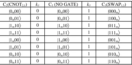
Table 2. All possible C3 output with C2(CNOT2,1) input.

C2(CNOT2,1) k3 C3 (NO GATE) k3 C3(SWAP1,3)

|0m00〉 0 |0m00〉 1 |000m〉

|0m01〉 0 |0m01〉 1 |100m〉

|1m10〉 0 |1m10〉 1 |011m〉

|1m11〉 0 |1m11〉 1 |111m〉

|1m00〉 0 |1m00〉 1 |001m〉

|1m01〉 0 |1m01〉 1 |101m〉

|0m10〉 0 |0m10〉 1 |010m〉

|0m11〉 0 |0m11〉 1 |110m〉

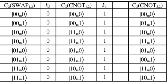
C2(SWAP1,2) will pass either from the CNOT1,2 gate, when k3 is equal to 0 or by

CNOT3,2 when k3 is equal to 1. The index 1,2 of CNOT gate defines the first qubit

as control and the second qubit as target. Thus, the CNOT1,2 gate inverts the

second qubit when the first qubit is equal to 1. Likewise, the index 3,2 of CNOT

gate defines the third qubit as control and the second qubit as target. Thus, the

CNOT3,2 gate inverts the second qubit when the third qubit is equal to 1. We have

selected the CNOT1,2 and CNOT3,2 gates to create diffusion to the data bit which is

found in the second qubit in the quantum states, | 12 1 1mk

k 〉, of Phase 2.

The output C3 that results from CNOT1,2 and CNOT3,2 quantum gates (see

Figure 1), denoted as C3(CNOT1,2) and C3(CNOT3,2) respectively, is represented

by Equation 4:

m k t and k

k m where k

t k

C = m > ∈ m = ⊕

1 1 2

1 1 1 2

1 1 1 1,2

m k t and k

k m where k

t k

C = m > ∈ m = ⊕

2 1 2

1 1 1 2

1 1 1 3,2

3(CNOT ) | , , , , {0,1}

Based on the third group of key element k3, all possible combinations of

C3(CNOT1,2) and C3(CNOT3,2) states are shown in Table 3:

Table 3. All possible C3 output with C2(SWAP1,2) input.

C3(CNOT3,2)

k3 C3(CNOT1,2)

k3 C2(SWAP1,2)

|00m0〉

1 |00m0〉

0 |00m0〉

|01m1〉

1 |00m1〉

0 |00m1〉

|10m0〉

1 |11m0〉

0 |10m0〉

|11m1〉

1 |11m1〉

0 |10m1〉

|01m0〉

1 |01m0〉

0 |01m0〉

|00m1〉

1 |01m1〉

0 |01m1〉

|11m0〉

1 |10m0〉

0 |11m0〉

|10m1〉

1 |10m1〉

0 |11m1〉

Phase 4: Non-Orthogonality

In Phase 4, the fourth group key k4 is responsible for leading the encrypted data to

non-orthogonality. The encrypted data derived from the second level of

encryption are states which are orthogonal. However, orthogonality is a property

which should be avoided so that the encrypted data are securely transferred

through the communication channel. Orthogonality permits states to be

distinguished and thus, phase 4 makes the outputs states non-orthogonal.

Non-orthogonality is a preferable property for PEA.

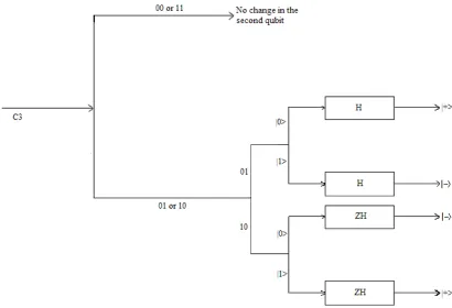
Non-orthogonality is achieved by using the fourth key, k4. According to

the key, k4, we change the second qubit in the following approach: If the key

element is 00 or 11, then we do not change the second qubit of state C3. Thus, the

second qubit remains in the state |0〉 or |1〉. However, when the key element is 01 or 10, then we perform the following computations to the second qubit: when the

key element has value equal to 01, we apply Hadamard (H) gate [10] to the

second qubit and the resulting output state is |+〉 if the input state is |0〉, or |-〉 if the input state is |1〉. If the key element is 10, we apply ZH gate [10] to the second qubit and the resulting output state is |-〉 if the input state is |0〉, or |+〉 if the input state is |1〉. We select the second qubit to be passed by H or ZH gates because in the second qubit there is the quantum representation of a data bit after Phase 3,

The Non-Orthogonality process is shown in Figure 2. For each output

C3(NO GATE), C3(SWAP1,3), C3(CNOT1,2), and C3(CNOT3,2), non-orthogonality

is also illustrated in Figure 1.

Figure 2. Non-Orthogonality Process

To prove that the utilization of Hadamard gates and ZH gates offers

non-orthogonality, we need to follow the next steps:

Firstly, it is known that Hadamard gate is given by Equation 5 [10]:

     

− =

1 1

1 1

2 1 ^

H (0)

It is also known that the matrix representations of the |0〉 and the |1〉 are given by Equation 6 [10]:

      = >

0 1 0

| and _

     = >

1 0 1

| (0)

From equations 5 and 6 we can calculate the following:

> + ≡ > + > =

      =            

− =

> (|0 |1 ) | 2

1 1 1

2 1 0 1

1 1

1 1

2 1 0 | ^ H

> − ≡ > − > =

      − =

           

− =

> (|0 |1 ) | 2

1 1 1

2 1 1

0

1 1

1 1

2 1 1 | ^ H

(0)

      − = 1 1 1 1 2 1 ^ H Z (0) and       = > 0 1 0

| and _

     = > 1 0 1

| . (0)

From equations 8 and 9 we can calculate the following:

> − ≡ > − > =       − =             − =

> (|0 |1 ) | 2 1 1 1 2 1 0 1 1 1 1 1 2 1 0 | ^ H Z > + ≡ > + > =       =             − =

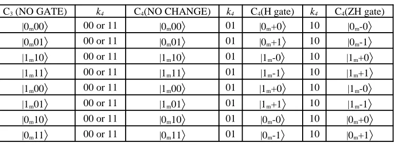
> (|0 |1 ) | 2 1 1 1 2 1 1 0 1 1 1 1 2 1 1 | ^ H Z . (0)

For input C3(NO GATE), the output C4 results from not changing the second qubit

of the input C3(NO GATE) or applying H / ZH quantum gates to the second qubit

of the input C3(NO GATE). These results denoted as C4(NO CHANGE), C4(H

gate) and C4(ZH gate) are represented by Equation 11:

11 00 } 1 , 0 { , , , , , | CHANGE)

(NO ₁1 ₁2 ₁1 ₁2 ₄

4 m k k where m k k when k or

C = > ∈ =

01 } 1 , 0 { , , , , , | gate)

(H ₁2 ₁1 ₁2 ₄

4 = m ± k > where m k k ∈ when k = C 10 } 1 , 0 { , , , , , | gate)

(ZH 2 ₄

1 1 1 2

1

4 = m k > where m k k ∈ when k =

C _∓ .

(0)

Based on the fourth group of key element k4,all possible combinations of C4(NO

CHANGE), C4(H gate) and C4(ZH gate) states are shown in Table 4:

Table 4. All possible C4 output with C3(NO GATE) input.

C3 (NO GATE) k4 C4(NO CHANGE) k4 C4(H gate) k4 C4(ZH gate)

|0m00〉 00 or 11 |0m00〉 01 |0m+0〉 10 |0m-0〉

|0m01〉 00 or 11 |0m01〉 01 |0m+1〉 10 |0m-1〉

|1m10〉 00 or 11 |1m10〉 01 |1m-0〉 10 |1m+0〉

|1m11〉 00 or 11 |1m11〉 01 |1m-1〉 10 |1m+1〉

|1m00〉 00 or 11 |1m00〉 01 |1m+0〉 10 |1m-0〉

|1m01〉 00 or 11 |1m01〉 01 |1m+1〉 10 |1m-1〉

|0m10〉 00 or 11 |0m10〉 01 |0m-0〉 10 |0m+0〉

|0m11〉 00 or 11 |0m11〉 01 |0m-1〉 10 |0m+1〉

For input C3(SWAP1,3), the output C4 results from not changing the second qubit

of the input C3(SWAP1,3), or applying H or ZH quantum gates to the second qubit

of the input C3(SWAP1,3). These results denoted as C4(NO CHANGE), C4(H gate)

11 00 }

1 , 0 { , , ,

, , | CHANGE)

(NO 2 ₄

1 1 1 1

1 2 1

4 k k m where m k k when k or

C = > ∈ =

01 }

1 , 0 { , , ,

, | gate)

(H ₁2 ₁1 ₁2 ₄

4 = k ± m> where m k k ∈ when k = C

10 }

1 , 0 { , , ,

, , | gate)

(ZH 4

2 1 1 1 2

1

4 = k m> where m k k ∈ when k =

C ∓

(0)

Based on the fourth group of key element k4,all possible combinations of C4(NO

CHANGE), C4(H gate) and C4(ZH gate) states are shown in Table 5:

Table 5. All possible C4 output with C3(SWAP1,3) input.

C3(SWAP1,3) k4 C4(NO CHANGE) k4 C4(H gate) k4 C4(ZH gate)

|000m〉 00 or 11 |000m〉 01 |0+0m〉 10 |0-0m〉

|100m〉 00 or 11 |100m〉 01 |1+0m〉 10 |1-0m〉

|011m〉 00 or 11 |011m〉 01 |0-1m〉 10 |0+1m〉

|111m〉 00 or 11 |111m〉 01 |1-1m〉 10 |1+1m〉

|001m〉 00 or 11 |001m〉 01 |0+1m〉 10 |0-1m〉

|101m〉 00 or 11 |101m〉 01 |1+1m〉 10 |1-1m〉

|010m〉 00 or 11 |010m〉 01 |0-0m〉 10 |0+0m〉

|110m〉 00 or 11 |110m〉 01 |1-0m〉 10 |1+0m〉

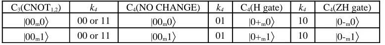
For input C3(CNOT1,2), the output C4 results from not changing the second qubit

of the input C3(CNOT1,2), or applying H / ZH quantum gates to the second qubit

of the input C3(CNOT1,2). These results denoted as C4(NO CHANGE), C4(H gate)

and C4(ZH gate) are represented by Equation 13:

11 00 }

1 , 0 { , , ,

, , | CHANGE)

(NO ₁1 ₁2 ₁1 ₁2 ₄

4 k m k where m k k when k or

C = > ∈ =

01 }

1 , 0 { , , ,

, , | gate)

(H ₁1 ₁2 ₁1 ₁2 ₄

4 = k ± k > where m k k ∈ when k = C

10 }

1 , 0 { , , ,

, , | gate)

(ZH ₁1 ₁2 ₁1 ₁2 ₄

4 = k k > where m k k ∈ when k =

C ∓

(0)

Based on the fourth group of key element k4,all possible combinations of C4(NO

CHANGE), C4(H gate) and C4(ZH gate) states are shown in Table 6:

Table 6. All possible C4 output with C3(CNOT1,2) input.

C3(CNOT1,2) k4 C4(NO CHANGE) k4 C4(H gate) k4 C4(ZH gate)

|00m0〉 00 or 11 |00m0〉 01 |0+m0〉 10 |0-m0〉

|11m0〉 00 or 11 |11m0〉 01 |1-m0〉 10 |1+m0〉

|11m1〉 00 or 11 |11m1〉 01 |1-m1〉 10 |1+m1〉

|01m0〉 00 or 11 |01m0〉 01 |0-m0〉 10 |0+m0〉

|01m1〉 00 or 11 |01m1〉 01 |0-m1〉 10 |0+m1〉

|10m0〉 00 or 11 |10m0〉 01 |1+m0〉 10 |1-m0〉

|10m1〉 00 or 11 |10m1〉 01 |1+m1〉 10 |1-m1〉

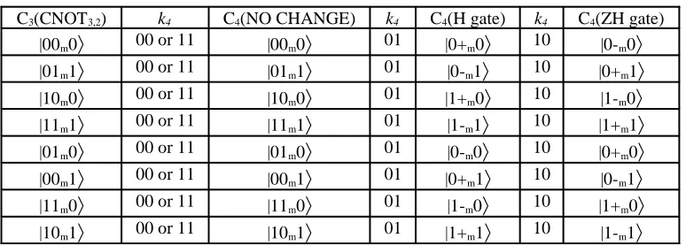
For input C3(CNOT3,2), the output C4 results from not changing the second qubit

of the input C3(CNOT3,2), or applying H / ZH quantum gates to the second qubit

of the input C3(CNOT3,2),. These results denoted as C4(NO CHANGE), C4(H

gate) and C4(ZH gate) are represented by Equation 14:

11 00 }

1 , 0 { , , ,

, , | CHANGE)

(NO ₁1 ₁2 ₁1 ₁2 ₄

4 k m k where m k k when k or

C = > ∈ =

01 }

1 , 0 { , , ,

, , | gate)

(H ₁1 ₁2 ₁1 ₁2 ₄

4 = k ± k > where m k k ∈ when k = C

10 }

1 , 0 { , , ,

, , | gate)

(ZH 4

2 1 1 1 2

1 1 1

4 = k k > where m k k ∈ when k =

C ∓

(0)

Based on the fourth group of key element k4,all possible combinations of C4(NO

CHANGE), C4(H gate) and C4(ZH gate) states are shown in Table 7:

Table 7. All possible C4 output with C3(CNOT3,2) input.

C3(CNOT3,2) k4 C4(NO CHANGE) k4 C4(H gate) k4 C4(ZH gate)

|00m0〉 00 or 11 |00m0〉 01 |0+m0〉 10 |0-m0〉

|01m1〉 00 or 11 |01m1〉 01 |0-m1〉 10 |0+m1〉

|10m0〉 00 or 11 |10m0〉 01 |1+m0〉 10 |1-m0〉

|11m1〉 00 or 11 |11m1〉 01 |1-m1〉 10 |1+m1〉

|01m0〉 00 or 11 |01m0〉 01 |0-m0〉 10 |0+m0〉

|00m1〉 00 or 11 |00m1〉 01 |0+m1〉 10 |0-m1〉

|11m0〉 00 or 11 |11m0〉 01 |1-m0〉 10 |1+m0〉

|10m1〉 00 or 11 |10m1〉 01 |1+m1〉 10 |1-m1〉

2.2. Decryption

All gates (CNOT gates, SWAP gates, H gates, ZH gates) used in the encryption

and non-orthogonality processes are unitary operators. Hence, the decryption is

the inverse process of the encryption using the pre-shared four group keys. The

decryption process takes place at the recipient side. Thus, the decryption process

Phase 1: Inverse process of Phase 4 of Encryption process

In Phase 1, the fourth group key k4 is responsible for the first level of decryption.

The recipient receives the non-orthogonal states (ciphertext) from the sender and

applies the same process with the one applied in the Phase 4 during encryption.

When the key element is 00 or 11 we do not change the second qubit of state C4

and thus, the second qubit remains in state |0〉 or |1〉. However, when the key element is 01 or 10, then we perform the following computations to the second

qubit of the ciphertext: If the key element has value equal to 01, we apply H gate

to the second qubit and the output state is |0〉 when the input state is |+〉, or |1〉 when the input state is |-〉. If the key element is 10, we apply ZH gate to the second qubit and the resulting output state is |0〉 when the input state is |-〉, or |1〉 when the input state is |+〉. Therefore, the output of this phase is the state C3 of the encryption process.

Phase 2: Inverse process of Phase 3 of Encryption process

In Phase 2, the third and second group keys k3, k2 are responsible for the second

level of decryption. The inputs of phase 2 are the outputs of the first level of

decryption. Here the recipient applies the same process with the process applied in

phase 3 during the encryption process. For example, when k2 is equal to 0, state C3

passes either by the path which has no gate for k3 equal to 0, or by SWAP1,3, for k3

equal to 1. When k2 is equal to 1 state C3 passes either by the CNOT1,2 gate for k3

equal to 0, or by CNOT3,2 for k3 equal to 1. Hence, the output of this phase is the

state C2 of the encryption process.

Phase 3: Inverse process of Phase 2 of Encryption process

In Phase 3, the second group of key element k2 is responsible for the third level of

decryption. The inputs of phase 3 are the outputs of the second level of

decryption. Same as before the receiver applies the same process with the one

applied in phase 2 during encryption. For example, when k2 is equal to 0, state C2

passes by the CNOT2,1 gate, but when k2 is equal to 1, state C2 passes by the

SWAP1,2 gate. Hence the output of this phase is the state C1 of the encryption

Phase 4: Acquisition of plaintext

In Phase 4, we obtain all the first qubits of each state that correspond to the

original bits and acquire the bit sequence of the original plaintext.

3. Security Analysis of PEA

To evaluate PEA we have conducted a security analysis to examine its resilience

to Trojan horse and eavesdropping attacks and to study its homogeneity and

perfect secrecy.

3.1. Homogeneity and Perfect Secrecy

It is essential an encryption algorithm to produce homogeneous ciphertexts and

ideally have perfect secrecy, i.e. the ciphertext gives no information about the

plaintext [20]. To prove that our algorithm is homogeneous and achieves perfect

secrecy, it is enough to show that the density matrix of n ciphertexts states related

to the n bits classical message is the identity matrix.

To prove it, let |ψwz〉 be the linear combination of all possible states with equal probability in the ciphertext set Cw (w=1, 2, 3), which corresponds to the zth bit of

message. The density matrices are calculated by Equation 15:

|ψ1z〉 〈ψ1z| = I |ψ2z〉 〈ψ2z| = I |ψ3z〉 〈ψ3z| = I (0)

The density matrix of n ciphertext states |ψ3〉 for a message which consists of n bits is given by Equation 16:

|ψ3〉 〈ψ3| = |ψ31〉 〈ψ31| ⊗|ψ32〉 〈ψ32|⊗|ψ33〉 〈ψ33|. . . ⊗|ψ3n〉 〈ψ3n| (0)

To calculate Equation 16, firstly it is required to calculate the outer product of

each element |ψ3i〉: |ψ31〉 〈ψ31|, |ψ32〉 〈ψ32|, |ψ33〉 〈ψ33|, |ψ34〉 〈ψ34|, |ψ35〉 〈ψ35|, |ψ36

〉 〈ψ36|, |ψ37〉 〈ψ37|, |ψ38〉 〈ψ38|

Then, it is required to calculate the tensor products of the above outer

001〉, |010〉, |011〉, |100〉, |101〉, |110〉, |111〉, can be also represented as vectors. By using vectors we can make simple calculations and prove that the ciphertext is

homogenous. For example, the vector representation of the first states |000〉 is given by Equation 17:

|000〉= |0〉 ⊗|0〉 ⊗|0〉= _

    

0 1

⊗ _     

0 1

⊗ _     

0 1

=

   

 

   

 

0 0 0 1

⊗ _     

0 1

=

          

 

          

 

0 0 0 0 0 0 0 1

(0)

Likewise, we can construct the rest of the states |001〉, |010〉, |011〉, |100〉, |101〉, | 110〉, and |111〉 as vectors.

According to Figure 1, when the output is given by C3 (NO GATE) we

have the following possible states:

Table 8. C3 (NO GATE) Output.

|0m00〉 |0m01〉 |1m10〉 |1m11〉 |1m00〉 |1m01〉 |0m10〉 |0m11〉

From Table 8, we have:

|ψ31〉=|0m00〉, |ψ32〉=|0m01〉, |ψ33〉=|1m10〉, |ψ34〉=|1m11〉, |ψ35〉=|1m00〉, |ψ36〉=|1m01〉, |ψ37〉=|0m10〉, |ψ38〉=|0m11〉.

Next, the outer products can be calculated by Equation 18:

|ψ31〉 〈ψ31| = |0m00〉 〈0m00| = eeT= E where

e = [1 0 0 0 0 0 0 0]T ,

E = Diag{1, 0, 0, 0, 0, 0, 0, 0}

(18)

Likewise, we can calculate all the outer products |ψ32〉〈ψ32|, |ψ33〉〈ψ33|, |ψ34〉〈ψ34|, | ψ35〉〈ψ35|, |ψ36〉〈ψ36|, |ψ37〉〈ψ37|, and |ψ38〉〈ψ38|.

According to Figure 1, when the output is given by C3(SWAP 1,3) we

have the following possible states:

Table 9. C3 (SWAP 1,3) Output.

From Table 9, we have:

|ψ31〉=|000m〉, |ψ32〉=|100m〉, |ψ33〉=|011m〉, |ψ34〉=|111m〉, |ψ35〉=|001m〉, |ψ36〉=|101m〉, |ψ37〉=|010m〉, |ψ38〉=|110m〉. The outer product of |ψ31〉 〈ψ31| is given by Equation 19:

|ψ31〉 〈ψ31| = |000m〉 〈000m| = eeT= E where

e = [1 0 0 0 0 0 0 0]T_,

E = Diag{1, 0, 0, 0, 0, 0, 0, 0}

(19)

Likewise, we can calculate |ψ32〉 〈ψ32|, |ψ33〉 〈ψ33|, |ψ34〉 〈ψ34|, |ψ35〉 〈ψ35|, |ψ36〉 〈 ψ36|, |ψ37〉 〈ψ37|, and |ψ38〉 〈ψ38|.

According to Figure 1, when the output is given by C3(CNOT1,2) we have

the following possible states:

Table 10. C3(CNOT1,2) Output.

|00m0〉 |00m1〉 |11m0〉 |11m1〉 |01m0〉 |01m1〉 |10m0〉 |10m1〉

From Table 10, we have:

|ψ31〉=|00m0〉, |ψ32〉=|00m1〉, |ψ33〉=|11m0〉, |ψ34〉=|11m1〉,

|ψ35〉=|01m0〉, |ψ36〉=|01m1〉, |ψ37〉=|10m0〉, |ψ38〉=|10m1〉.

The outer product of |ψ31〉 〈ψ31| is given by Equation 20:

|ψ31〉 〈ψ31| = |00m0〉 〈00m0| = eeT= E

where

e = [1 0 0 0 0 0 0 0]T ,

E = Diag{1, 0, 0, 0, 0, 0, 0, 0}

(0)

Likewise, we can calculate |ψ32〉 〈ψ32|, |ψ33〉 〈ψ33|, |ψ34〉 〈ψ34|, |ψ35〉 〈ψ35|, |ψ36〉 〈 ψ36|, |ψ37〉 〈ψ37|, and |ψ38〉 〈ψ38|.

According to Figure 1, when the output is given by C3(CNOT3,2) we have

the following possible states:

Table 11. C3(CNOT3,2) Output.

From Table 11, we have:

|ψ31〉=|00m0〉, |ψ32〉=|01m1〉, |ψ33〉=|10m0〉, |ψ34〉=|11m1〉, |ψ35〉=|01m0〉, |ψ36〉=|00m1〉, |ψ37〉=|11m0〉, |ψ38〉=|10m1〉.

The outer product of |ψ31〉 〈ψ31| is given by Equation 21:

|ψ31〉 〈ψ31| = |00m0〉 〈00m0| = eeT = E where

e = [1 0 0 0 0 0 0 0]T ,

E = Diag{1, 0, 0, 0, 0, 0, 0, 0}

(0)

Likewise, we can calculate |ψ32〉 〈ψ32|, |ψ33〉 〈ψ33|, |ψ34〉 〈ψ34|, |ψ35〉 〈ψ35|, |ψ36〉 〈 ψ36|, |ψ37〉 〈ψ37|, and |ψ38〉 〈ψ38|.

We notice that the first output (|00m0〉) given by C3(CNOT1,2) (see Table 10) is the same with the first output (|00m0〉) given by C3(CNOT3,2) (see Table 11). Consequently, the linear combination |ψ31〉corresponds to the state |00m0〉is the same for the both cases. Thus, equation (20) and equation (21) are identical.

According to the assumption that k1, k2, k3, k4, are uniformly distributed

and based on the above matrices of the outer products, we can calculate the tensor

products and obtain the following density matrix:

|ψ3〉 〈ψ3| = |ψ31〉〈ψ31| ⊗|ψ32〉 〈ψ32|⊗|ψ33〉 〈ψ33|. . . ⊗|ψ3n〉 〈ψ3n| = I (0)

Equation 22 demonstrates that the ciphertext is homogeneous and has perfect

secrecy, since the density matrix is equal to the identity matrix.

3.2. Trojan horse attacks tolerance

The Trojan horse attacks are the most serious threats to computer networking

security. However, the proposed algorithm is tolerant against Trojan horse attacks.

If a Trojan horse, denoted as T, has invaded in the sender or the recipient in order

) 1 1 | 0 1 | 1 0 | 0 0 | 1 1 | 0 1 | 1 0 | 0 0 | 0 1 | 0 0 | 1 1 | 1 0 | 1 1 | 1 0 | 0 1 | 0 0 | 1 0 | 0 0 | 1 1 | 0 1 | 1 1 | 0 1 | 1 0 | 0 0 | 1 0 1 | 0 1 1 | 1 0 0 | 0 1 0 | 1 1 1 | 0 0 1 | 1 1 0 | 0 0 0 | 0 1 1 | 0 1 0 | 1 0 1 | 1 0 0 | 1 1 1 | 1 1 0 | 0 0 1 | 0 0 0 | 1 1 0 | 0 1 0 | 1 0 1 | 0 0 1 | 1 1 1 | 0 1 1 | 1 0 0 | 0 0 0 (| 48 1 ) ( | ? || ? ? || || ? || ? || ? ? || || ? || || ? || ? || ? ? || ? ? || ? || ? || ? || || ? || ? || ? ? || ? ? || || ? || || || || || || || || || || || || || || || || || || || || || || || || || || || || || || || || || || || || 4 > + + > − + > + + > − + > − + > + + > − + > + + > − + > − + > + + > + + > − + > − + > + + > + + > − + > − + > + + > + + > − + > − + > + + > + + > + > + > + > + > + > + > + > + > + > + > + > + > + > + > + > + > + > + > + > + > + > + > + > = ⊥ ⊥ ⊥ ⊥ ⊥ ⊥ ⊥ ⊥ ⊥ ⊥ ⊥ ⊥ ⊥ ⊥ ⊥ ⊥ ⊥ ⊥ ⊥ ⊥ ⊥ ⊥ ⊥ ⊥ ⊥ ⊥ ⊥ ⊥ ⊥ ⊥ ⊥ ⊥ ⊥ ⊥ ⊥ ⊥ ⊥ ⊥ ⊥ ⊥ ⊥ ⊥ ⊥ ⊥ ⊥ ⊥ ⊥ ⊥ ⊥ ⊥ ⊥ ⊥ ⊥ ⊥ ⊥ ⊥ ⊥ ⊥ ⊥ ⊥ ⊥ ⊥ m m m m m m m m m m m m m m m m m m m m m m m m m m m m m m m m m m m m m m m m m m m m m m m m i T ψ (0)

In Equation 23, we have used three symbols. The symbol || is the information

obtained by the Trojan horse when the quantum state is |0〉. The symbol ⊥ is the information obtained by the Trojan horse when the quantum state is |1〉. Whereas, the symbol ? is the information obtained by the Trojan horse when the quantum

state is |+〉 or |-〉. It means that when the state is |+〉 or |-〉 due to non-orthogonality that is applied in the fourth phase of encryption process, the Trojan horse can not

decide which the valid state is. Moreover, according to the design of encryption

algorithm, the quantum representation of a data bit can be in the first qubit or in

the second qubit or in the third qubit. Thus, the Trojan horse is able to take any

information related to the plaintext as well as which qubit is related to the ancilla

qubit.

3.3. Eavesdropping attacks tolerance

According to the design of PEA, the ciphertext states are non-orthogonal leading

the ciphertext states to be undistinguishable by an eavesdropping attacker. The

non-orthogonality is applied in the fourth phase of encryption process and we can

prove it by calculating the 〈ψ4i | ψ4i〉. If the value of inner product 〈ψ4i | ψ4i〉 is larger than 0, it means that the ciphertext states are non-orthogonal [10].

represent the states |0+0〉, |0-0〉, |0+1〉, |0-1〉, |1+0〉, |1+1〉, |1-0〉, and |1-1〉 as vectors. For example, the vector representation of |0+0〉is given by Equation 24:

|0+0〉= |0〉 ⊗|+〉 ⊗|0〉= _

     0 1 ⊗             2 1 2 1 ⊗ _      0 1 =                   0 0 2 1 2 1 ⊗ _      0 1 =                               0 0 0 0 0 2 1 0 2 1 (0)

Likewise, we can calculate |0-0〉, |0+1〉, |0-1〉, |1+0〉, |1+1〉, |1-0〉, and |1-1〉.

Hence, according to Equations 17, 25 and their further calculations we have:

                                                        + + + + =                                                                           − − +                                     +                                     − − +                                     +                           = > 1 1 2 1 2 1 1 1 2 1 2 1 16 1 2 1 2 1 2 1 2 1 0 0 0 0 2 1 2 1 2 1 2 1 0 0 0 0 0 0 0 0 2 1 2 1 2 1 2 1 0 0 0 0 2 1 2 1 2 1 2 1 1 1 1 1 1 1 1 1 48 3

|

ψ

Next, we can calculate the inner product 〈ψ4i | ψ4i〉 as shown in Equation 26:

[

]

(

)

32 1 1 1 2 1 2 1 1 1 2 1 2 1 1 1 2 1 2 1 1 1 2 1 2 1 256 1 ψ |

ψ4i 4i = +

(

)

1

ψ

|

ψ4i 4i >= + >

< (0)

By proving that the value of inner product <ψ4i |ψ4i > is larger than 0, it means that the ciphertext states are non-orthogonal.

4. Conclusion

To our knowledge there are still not many good and feasible quantum encryption

algorithms proposed. With the rapid progress of quantum information theory and

technology, quantum information comes into real life quietly. When the quantum

computers come true some day, it will be necessary and not always possible to

transfer the existing encryption algorithms into quantum information. Based on

the basic principle of quantum computation, a quantum cryptographic algorithm

to encrypt the classical binary bits was proposed. The security of the encryption

algorithm was analyzed in detail. It was shown that the proposed algorithm can

prevent quantum as well as classical attacks.

PEA has several properties. First of all, no quantum state is pre-shared or

stored making PEA possible and efficient in real applications. Second, it achieves

perfect secrecy with the condition that the key is uniformly distributed. Third,

both encryption and decryption are based on simple quantum computation, and

particularly on a combination of the quantum CNOT and SWAP gates. Fourth, its

implementation is feasible with the existing technology. At last, the same

algorithm can be extended to encrypt quantum information.

References

[1] Nanrum Zhou, Guihua Zeng, Yiyou Nie, Jin Xiong and Fuchen Zhu, "A

novel quantum block encryption algorithm based on quantum computation",

Physica A: Statistical Mechanics and its Applications, Volume 362, Issue 2, 1

April 2006, Pages 305-313

[2] Osamu Hirota, Masaki Sohma, Masaru Fuse, Kentaro Kato, "Quantum

stream cipher by the Yuen 2000 protocol: Design and experiment by an

[3] N. Gisin, S. Wolf, "Quantum Cryptography on noisy Channels:

Quantumversus Classical Key-Agreement Protocols", The American Physical

Society, 1999

[4] Rob Pike, "An Introduction to Quantum Computation and Quantum

Communication", Bell Labs, Lucent Technologies, June 23, 2000

[5] Yoshihiro NAMBU and Hideo KOSAKA, "Introduction of Quantum

Cryptography and Its Development", NEC Res. & Develop., Vol 44, No. 3,

July 2003

[6] Emanuel Knill, Raymond Laflamme, Howard N. Barnum, Diego A.Dalvit,

Jacek J. Dziarmaga, James E. Gubernatis, Leonid Gurvits, Gerardo Ortiz,

Lorenza Viola, and Wojciech H. Zurek, "Quantum Information Processing: A

hands-on primer", Los Alamos Science Number 27, 2002

[7] Ari Y. Benbasat, "A Survey of Current Optical Security Techniques", MIT

Media Lab, April 15, 1999

[8] Steven Linton, "Quantum Cryptography-Quantum Key Distribution", July

13, 2003

[9] Dheera Venkatraman, "Methods and implementation of quantum

cryptography", MIT Department of Physics, 27 April 2004

[10] Michael A. Nielsen and Isaac L. Chuang, Quantum Computation and

Quantum Information, Cambridge Press, 2004

[11] X. Y. Li, H. Barnum, "Quantum authentication using entangled states",

International Journal of Foundations Computer Science, Volume 15, Issue 4,

2004, Pages: 609-617.

[12] P.O. Boykin and V. Roychowdhury, "Optimal encryption of quantum

bits", Physics Review A, Vol. 67, 2003.

[13] H. Bechmann-Pasquinucci and N. Gisin, "Intermediate states in quantum

cryptography and Bell inequalities", Physics Review A, Vol 67, 062310, 2003

[14] N. Zhou, G. Zeng, "Progress on Cryptography", The Kluwer

International Series in Engineering and Computer Science, Kluwer Academic

Publishers, Boston, 2004, Pages: 195–200.

[15] N. Zhou, G. Zeng, "A realizable quantum encryption algorithm for

qubits", China Physics, Vol. 14, Issue 2164, 2005

[16] G. Benenti and G. Casatti, Principles of Quantum Computation, vol. I:

[17] Justin Mullins, "Making Unbreakable Code", IEEE Spectrum, May 2002.

[18] A.M. Steane, E.G. Rieffel, "Beyond Bits: The Future of Quantum

Information Processing", IEEE Computer, January 2000.

[19] William Stallings, Cryptography and Network Security Principles and

Practices, Prentice Hall, November 2005.

[20] A. J. Menezes, S. A. Vanstone, and P. C. Van Oorschot, Handbook of