Multi dimensional data scaling – dynamical cascade approach

Multi-dimensional data scaling – dynamical cascade

approach

Milan Jovovic, Geoffrey Fox

Indiana University

ABSTRACT

In this report a multi-dimensional data scaling approach is proposed in data mining and knowledge discovery applications. We derive the method based on an analogy to the physical computation of signal distortion. A dynamical cascade computation diagrams result from the statistical physics model computation in the free energy decomposition. We assess the scale invariance of various data sets, such as with the image motion sequences, and with the high dimensional chemical data sets. Theoretical model of error propagation is given by the numerical computational schemes. Statistical mapping of the data is analyzed through dynamical cascades, as a way of approaching its coding and control data structure. We show how it correlates by segmenting set of chemical compounds observations in a high dimensional property space. The proposed algorithm, also, is suitable for the implementation in parallel computer architectures. An example implementation on the multicore processors is given in the end of this report.

1.

INTRODUCTION

A multifractal model formalism is derived in the “Thalweg ARC.” project report [12], to explain the decomposition of image sequences into the singular data sets. The partition function describes the probabilistic model of data clusters and is analyzed as a multifractal measure in the method. Singularity analysis of computational maps of clustering vectors is derived to describe the computational means of decomposing the image information into different singular sets. We show also that the propagation of information in image sequences is governed by the scale-space wave equation, therefore enabling us to treat singular frequencies of data clusters in an unified way, both in space and in time.

Contextual information of the spatial coherency of data is used in the segmentation process in the hierarchical scale computation of feature vectors. The spatial segmentation of images is performed while using the Green's function, parameterized with the scale parameter, as the integration function in the segmentation process. The scale information is evaluated by conjoining the two parameters: the scale parameter β of the signal distortion, and the spatial scale parameter r. A larger extent of spatial integration of the motion information is used on a larger scale, while it

becomes effectively more local in space as we decrease the scale of segmentation.

Distinct singular features are segmented on a certain scale and the least singular feature become segmented in two spatial windows with the Laplacian system regularity constraints, in the hierarchical scale computation. Accordingly, the reconstruction formula is derived based on the Laplacian system of the diffusion of the residual information from the most singular sets. This gives us an effective way of compressing and progressive coding of the information in image sequences. The binary tree data structure of the clustering parameters is suitable in the coding schemes that use the hierarchical structure of the binary images of the spatial distribution of cluster windows, along with the feature vectors and residual image information that make up for the point feature vector estimation.

We give here a derivation of the computational scheme for a 2-dimensional case, like in image sequences. We then consider a dynamical coupling and the energy exchange between 3 clusters computed. Corresponding statistical maps are analyzed w.r.t. the dimensionality of the eigenvalue decomposition of the clusters‟ covariances.

The results are shown for the chemical compounds in the 155 properties dimensional data set. Projections along the most singular components are computed in 1 and 2 dimensional statistical maps.

2.

METHOD

Variational data distributions

We define a cluster of data points here with its computed cluster vector representative y, and the selected group window of computation, W. Let d(x, y) denotes a distortion measure introduced to a data point x by the representation y. The distortion energy, or variance V of a cluster is defined by:

   

,

.





W

d

x

y

P

x

V

 

 



log



,

min

max/





W

P

x

P

x

subject to:





   

_,

_and



 



₁

_,

W W

d

x

y

P

x

P

x

V

is the Gibbs distribution:

 

     ,

,

, ,



       





W y x d y x d y x d

e

e

Z

e

x

P

_  

and

 

     ,

,

, ,



       





W y x d y x d y x d

e

e

Z

e

x

P

_  

respectively, where Z

-and Z+ are the partition functions, and - and + are the

corresponding Lagrange‟s multipliers.

Covariance differentiability and a scale-space

computing approach

The nonlinear dynamics of clustering, in this work is derived from the model of “free energy”, originally used in statistical physics to model different complex systems. The free energy describes the state of a cluster for a given parameter ,





1

log

_/

.

/

/ 

  







Z

F

_r





The parameter  is inversely proportional to temperature (=1/T), in physical analogy. The equilibrium states are computed to minimize the energy exchange among clusters for a given spatial distribution of the clusters.

The distortion measure, applied in the algorithm, is chosen to be the linear constraint equation on the motion vector

v



, also known as the extended optical flow constraint equation:

 

,

)

(

2

2

_I

_I

_v

_Idiv

_v

z

d





_t











which provides the mass conservation principle [1]. In this work the coherency of data is estimated with its Green's function, to control the smoothness of the optical flow adaptively in the scale.

The constrained equation of motion for a coupled pair of clusters is given by:











































F

v

F

v

F

v

v

F

v

F

v

1 1 2 2 2 2 2 1 1 1

















where the upper sign corresponds to the cooling part and lower to the melting part of the algorithm.

This system of equations can be analyzed by the series expansion of the system's free energies:

















 

2.

2 1 2 1 1 2 2 1 2 2 2 2 2 2 2 1 2 1 1 2 2 1 2 2 2 2 2 1 1 2 2 2 2 2 2 1 1 2 2 1 2 2 2 1 1 1 2 2 2 1 1 1 1 2 2 1 2 1                                                                        











































F F F F v v v F v F v F v F v v F F v v F v v F F F F F F T                 

This gives an update formula for the parameter β:

, 2 1 1 2 1 1 2 2 2 2 2 1 1 2 1 2 2 2 2 2 2 2 1 2 2 2 2 2 2 1 1 2 1 1 2 1























                      F v v F v v v F v F v v F v v v F v T T T T            

for the cooling part of the algorithm, and

, 2 1 1 2 1 1 2 2 2 2 2 1 1 2 1 2 2 2 2 2 2 2 1 2 2 2 2 2 2 1 1 2 1 1 2 1























                      F v v F v v v F v F v v F v v v F v T T T T            

for the melting part.

Note that this way we keep the integral:



















S S

d

v

V

v

d

F

dU



0

,







(7)



1



₂

.

2 2 2

2 1

1 2 2 2

2 2 2

2 1

1 2 2

v

F

v

F

v

F

v

F

















































Λ

Λ



D

For

0







1

the eigenvalues of the determinant of the map have negative values if the Hessians of the free energies, F1 and

F2, are positive definite, what gives a condition of numerical

stability of the coupled system‟s equations.

Scale-space pathways: resonance computing

Singularity of data clusters is evaluated by the means of the scalability of the maps of feature vector representatives in scale space. For a given maximal value of the distortion energy the minimal number of singularity manifolds is obtained in the hierarchical scale computation.

For a given cluster, the partition function

Z

 



,

r

describes the distribution of the data points with respect to the cluster vector representative. The scale information is evaluated by conjoining the two parameters: the signal energy distortion scale parameter β, and the spatial scale parameter r, which equals to the number of data points inside the spatial window of computation W. For a given point distortion measure of the signal,

z

2



d

 

x



,

y



, the partition function is written by:

 

_

_



W z sign

r

r

Z



,

2

and, a data point belongs to the cluster in probability, with the probability density function:

Z

r

P

z sign 2



The partition function can be conveniently written as:

 





( 1)





0  

.

 

 



  





sign F sign V sign V d

r

r

r

Z

This function is a multifractal measure, giving a way of decomposing the signal into feature vector clusters ordered by the singularity exponents, H=2βV < 1, and singular frequency factors, F/V < 1, as written in:

.

2 1 _

     



V F H

r

Z

The nonlinear dynamics of clustering is governed by the two energy functions. For a given cluster its free energy, and the distortion energy is defined by:

 







_

 

W

r

Z

V

d

x

y

P

v

F



,

1

log

,



,



.





We relate the mechanism of the multifractal decomposition of the signal to the stability analysis of the map.

The stability condition of this map is given by the relation: 2βV <

1. We limit the singularity exponent of the clusters with the maximal value H, by splitting that cluster in two for which the condition is reached: 2βcV = H, at the critical value of the scale

parameter βc.

Interesting points of observation become the “signal energy levels”:

F – V = const., (A.1)

and its propagation in time. The time derivative of this equation becomes:

v

V

F

v

V

v

V

F

V

F

V

V

F





















































 

















































 

log

1

log

1







_(A.2)

The Green‟s formula:















S

_v

d

V

v

d

F

,

0









as well as, the accompanying wave equation:

,

2 2 2

V

F











are used in the computational scheme for the estimation of the clustering parameters, and are still part of the ongoing research.

At the “signal scale equilibrium” _0

 



F _{, an isolated cluster}

can be modeled by the equations:

,

2_V

V _{ }





_



and,

















S

S

_V

d

v

V

d

v

V

.

0

2 2







_

The Green‟s function gives a model of spatial coherency of information for a data cluster:

 

,

₂

,

2

V

V

v

G













[image:4.612.71.531.117.252.2] [image:4.612.84.513.331.460.2]

(a) (b) (c)

Figure 1: Clustering of chemical data: 1225 observations in 155 dimensional property space. Statistical maps projections along the most singular components: (a) 1-dimensional, and (b) 2-dimensional. The observations are labeled with „1‟ and „2‟ to indicate a membership to the corresponding clusters. The difference in the membership labels in (a) and (b) is shown in figure 1.(c).

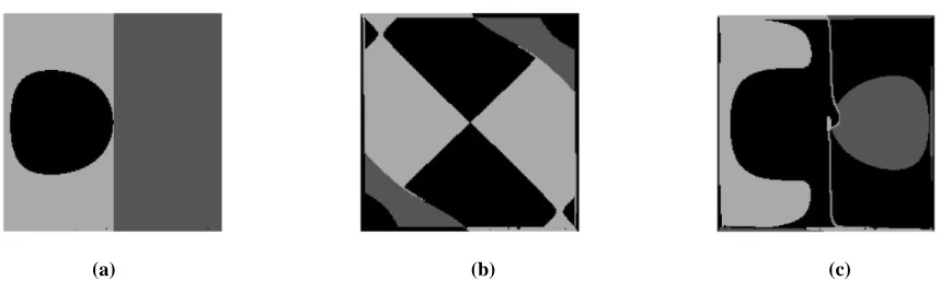
(a) (b) (c)

Figure 1: Clustering of the expanding ball image sequence. 3 clusters statistical maps projections along the singu lar components with: (a) divergence, (b) rotor, and, (c) divergence and rotor point segmentation.

3.

RESULTS

A dataset of 1236 compounds with 155 real-valued descriptors is used as a test case. The observations on the solubility of the compounds are analyzed in the segmentation algorithm. In the 1-dimensional case, the 1236 compounds are segmented in two groups with: N1 = 226, N2 = 1010 groups‟ members.

Corresponding clusters‟ variances are: V1 = 25x108, and V2 =

30x108, respectively. The resulting distribution of the data is shown in Figure 1(a).

In the 2-dimensional case we computed spatial map out of the 2 most singular components of the data. 1225 compounds were segmented in two groups with: N1 = 158, N2 = 1067 members.

And the resulting variances of the groups decreased as: V1 =

19x108, and V2 = 28x108, respectively. The resulting clusters‟

membership distribution of the data is shown in Figure 1(b). The difference in clustering as in (a) and (b) is shown in Figure 1.(c).

A test image sequence of an expanding ball is used as an example pattern for 2-dimensional signal decomposition. The statistical maps of the clusterized 3 image segments are shown in Figure 2. Differential operators: divergence, rotor, and a combination of the two are used for clustering data. The resulting membership distributions of data points are shown on Figures 2.(a-c) for these operators, respectively.

4.

CONCLUDING REMARKS

The Green's function expresses spatial coherency of data clusters and is used as an integration function for the segmenting data by applying local operators. In the method proposed, a decomposition in harmonic data sets is achieved by hierarchical scale computation. We use dynamical cascade diagrams to form a knowledge base discovered in the data, by this method.

We have run the algorithm only by applying the solubility as an additional property value in the data set. The improvements can be achieved by running the differential version segmentation on the solubility property. The associated structure diagrams can be used to relate different subsets of property values, and therefore making a knowledge base suitable for coding and control purposes.

We intend to investigate this tool in data mining applications – its coding and control structure implementation. The optimization of the space-energy exchange step along with the refinement of our numerical schemes is a part of our ongoing research work, as well.

ACKNOWLEDGEMENT

This work has been performed in the Pervasive Technology Labs' - Community Grids Lab, at the Indiana University.

5.

APENDIX

Main: decomposition – basic algorithm: Kmax= 3

1. Divide data evenly: N/Np to each core, i(p) and c = 1, indexed

Start with: Couple = 0.

2. For K



Kmax // Recursive procedure

3. Dogradual descentuntilresonate

Covar_project (); //Compute parameters: 3D + 2*dcov singular

components

Cls_map (+, -, Space); // Adjust with Green‟s functions

For all the clusters:

Cls_equilib (Sign =  1,Couple); // Equilibrate clusters

For all the clusters:

Cls_covar (Sign =  1); // Covariance computing

Cls_svmdcmp (Sign =  1); // Singular values decomp.

4. Test stability

IF the most spatially coherent cluster unstable

Split in 2 clusters, K++

ELSE IF a cluster empty

Merge in 1, K--

ELSEResonance

Cls_equilib (Sign, Coupling)

Do gradual descent until converge for all the clusters with partial sums:

1. Parallel_Sum_1 (p,

y



_c)

For all the clusters c:

 2

1 * xi yc

T Sign c

i

e

 _





 

 





p i

c i c

p

Z



,

and

 





 

c i p

i

i c

c

p

y

x

g















2. Sequential_update_1 ( )

 

 

*

(

1

,

)

*

couple

p c p

c c

c

y

T

Coupling

Sign

p

Z

p

g

Sign

y

y



















Cls_covar (Sign);

1. Parallel_Sum_2 (p,

y



_c, CCc)





2

1 * xi yc

T Sign c

i

e

 _





 







 









p i

c i d i d c d i d c c

d

d

p

y

x

y

x

CC

1 1 2 2



2 1,

 

 





k i p k i

p

Z



2. Sequential_update_2 ( )

 

 







p p

c c

p

Z

p

CC

CC

6.

REFERENCES

[1]

D.Bereziat, and J-P.Berroir, “Motion Estimation on Metereological Infrared Data using Total Brightness Invariance Hypothesis,” Environmental Modeling System, 2000.

[2]

M.Pierce, G.C.Fox, et al. “Smart Mining of Drug Discovery Information: 1. A web service and workflow infrastructure ,” 2006.

[3]

R.Courant, and D.Hilbert, Methods of Mathematical Physics, John Wiley & Sons, New York, 1962.

[4]

U.Grenander, and M.Miller, Pattern Theory: From Representation to Inference, Oxford University Press, 2007.

[5]

F.Hoppensteadt, and EIzhikevich, “Neural Computations by

Networks and Oscillators,” IJCNN, vol. 4, p. 4041, 200.

[6]

B.K.P.Horn, and B.G.Schunk, “Determining Optical Flow,”

Artificial Intelligence, vol. 17, pp. 185-203, 1981.

[7]

E.T.Jaynes, “Information theory and statistical mechanics,” in Papers on probability, statistics and statistical physics (R.D. Rosenkrantz, ed.), Kulwer Academic Publishers, 1989.

[8]

M.Jovovic, “A Markov random fields model for describing unhomogeneous textures: generalized random stereograms,”

IEEE Workshop Proceedings on Visualization and Machine Vision, and Biomedical Image Analysis, Seattle, 1994.

[9]

M.Jovovic, “Image segmentation for feature selection from

motion and photometric information by clustering,” SPIE Symposium on Visual Information Processing V, Orlando, 1996.

[10]

M.Jovovic, “A multiscale processing of data streams,” (in English) Informacione Tehnologije IV, Zabljak, Yugoslavia 1999.

[11]

M.Jovovic, S.Jonic, D.Popovic, “Automatic synthesis of synergies for control of reaching - hierarchical clustering,”

Med. Eng. and Physics, vol. 21/5, pp. 325-337, 1999.

[12]

M.Jovovic, “Space-Color Quantization of Multispectral

Images in Hierarchy of Scales,” ICIP01, vol. I, pp. 914-917, Thessaloniki, Greece, 2001.

[13]

M.Jovovic, H.Yahia, I.Herlin, “Hierarchical scale decomposition of images – singular feature analysis,”

Technical report, INRIA, 2003.

[14]

M.Jovovic, “Texture segmentation by 2-layers recurrent dynamics,” XXVIIIth International Symposium in

COMPUTATIONAL NEUROSCIENCE, Montreal. 2006.

[15]

K.Rose, E.Gurewitz, and G.C.Fox, “A Deterministic Annealing Approach to Clustering,” Pattern Recog. Lett.

vol.11, pp. 589-594, 1990.

[16]

A.Turiel, and A. del Pozo, “Reconstructing Images From Their Most Singular Fractal Manifold,” IEEE Trans. Image Processing, vol. 11/4, pp. 345-350, 2002.