Nanobubbles in bulk

(1)

Nanobubbles in Bulk

Muidh Hamed Alheshibri

May 2019

A thesis submitted for the degree of Doctor of Philosophy in Physics Research School of Physics and Engineering

(2)

(3)

Declaration

This thesis is an account of my own original research work, undertaken between March 2015 and May 2019 at the Department of Applied Mathematics in the Research School of Physics

and Engineering at the Australian National University.

To the best of my knowledge, this thesis contains no material previously published or written

by another person, except where due reference is made in the text.

(4)

(5)

Acknowledgement

First and foremost, I am greatly thankful to my supervisor Professor Vincent Craig for his support, enthusiasm, and encouragement throughout my PhD studies. This thesis would have

not been completed without his guidance, critical comments, and fruitful ideas. Working in his group has been a rewarding experience and I am eternally grateful to him for this opportunity.

I would also like to thank the Imam Abdulrahman Bin Faisal University and the Saudi Arabian Cultural Mission for the financial support I have received from them during my PhD studies.

I am grateful to Mr. Tim Sawkins at the Department of Applied Mathematics for his

contribution in designing the external pressure apparatus presented in this thesis.

I am also grateful to Dr. Victoria Coleman of the Nanometrology group in the Australian

National Measurement Institute for access to Archimedes apparatus and assistance during early stages of this project.

I would like to further extend my thanks to my fellow students and post-docs including Marie Jehannin, Namsoon Eom, Virginia Mazzini, Matthew Quinn, Zhu Xiaolong, Jane Qian and

E-Jen Teh.

(6)

(7)

Abstract

Currently, the existence of long-lived sub-micron bubbles in solution is not widely accepted as they should dissolve on a timescale of 1-100 microseconds, calculated through the use of a

widely accepted theory of bubble dissolution. Despite this, bulk nanobubbles are reported to have applications in different fields, such as water treatment and remediation, seed germination, surface cleaning, froth flotation, and ultrasound imaging. It is therefore important to develop

methods to test if nanoparticle dispersions contain nanobubbles.

Here, two methods are developed that are able to distinguish long-lived nanobubbles from nanoparticles. Firstly, the mean particle density of nanoparticles in a dispersion is determined. Secondly, the influence of external pressure on the size of nanoparticle dispersions is measured.

As the density and compressibility of a gas are very different to the density and compressibility of liquids and solids, these methods can differentiate between nanobubbles and other

nanoparticles.

The first part of my thesis focuses on nanobubbles that are armoured with a coating of insoluble surfactants. A novel technique for particle characterization that has the ability to distinguish positively buoyant particles (less dense than the solvent) from negatively buoyant particles

(8)

shell, which shields the bubble contents from some of the external pressure up to ~ 0.8 atm.

The presence of lipids of low solubility at the nanobubble-solution interface effectively results in a negative Laplace pressure, which stabilizes these nanobubbles against dissolution.

Having developed protocols that can be used to demonstrate the existence of bulk nanobubbles, these methods were then applied to different systems reported to contain nanobubbles. These

include nanoparticles produced by mechanical means, the mixing of ethanol and water and nitrogen supersaturation by chemical reaction. It was confirmed that nanoparticles were

produced in these systems. However, the measured density of these nanoparticles was inconsistent with the nanoparticles being gas filled. Furthermore, the external pressure had only a minimal effect on the size of these nanoparticles. These experiments reveal that processes that

lead to bubble formation can produce nanoparticles that result from the accumulation of material at the interface of the dissolving bubbles.

The results of this study demonstrate that the candidate nanoparticles investigated here are not

nanobubbles unless they are coated with insoluble materials and casts doubt on many reports of long-lived nanobubbles in bulk. Many researchers have reported the production of stable long-lived nanobubbles in bulk without providing direct evidence that the nanoparticles being

(9)

Publications and Presentations

Publications included as part of this thesis

1- M. Alheshibri, J. Qian, M. Jehannin, V.S.J. Craig, A History of Nanobubbles, Langmuir. 32 (2016) 11086–11100. doi:10.1021/acs.langmuir.6b02489.

2- M. Alheshibri, V.S.J. Craig, Differentiating Between Nanoparticles and Nanobubbles by Evaluation of the Compressibility and Density of Nanoparticles, J. Phys. Chem. C.

122 (2018) 21998–22007. doi:10.1021/acs.jpcc.8b07174.

3- M. Alheshibri, V.S.J. Craig, Armoured nanobubbles; ultrasound contrast agents under pressure, J. Colloid Interface Sci. 537 (2019) 123–131. doi:10.1016/j.jcis.2018.10.108.

4- M. Alheshibri, V.S.J. Craig, Generation of nanoparticles upon mixing ethanol and water; Nanobubbles or Not?, J. Colloid Interface Sci. 542 (2019) 136–143.

doi:10.1016/J.JCIS.2019.01.134.

5- M. Alheshibri, M. Jehannin, V. Coleman,V.S.J. Craig, Does Gas Supersaturation by a Chemical Reaction Produce Bulk Nanobubbles?, J. Colloid Interface Sci. 554 (2019)

(10)

2- M.H. Alheshibri, N.G. Rogers, A.D. Sommers, K.F. Eid, Spontaneous movement of

water droplets on patterned Cu and Al surfaces with wedge-shaped gradients, Appl. Phys. Lett. 102 (2013) 174103. doi:10.1063/1.4802926.

Oral Conference Presentations

1- M. Alheshibri and V.S.J. Craig. “The Puzzling Existence of Nanobubbles in Aqueous Solution". The 8th Biennial Australian Colloid Interface Symposium 2017. Coffs

Harbour, NSW, Australia.

2- M. Alheshibri and V.S.J. Craig. “Novel Approaches for the Characterization of Bulk Nanobubbles: A Step towards Solving the Puzzling Existence of Nanobubbles in

Aqueous Solution ". The 31st Australian colloid and surface science student conference 2018. Warrnambool, Victoria, Australia.

3- M. Alheshibri and V.S.J. Craig. “Novel Approaches for the Characterization of Bulk Nanobubbles: A Step towards Solving the Puzzling Existence of Nanobubbles in Aqueous Solution ". Conference on Nanobubbles, Nanodroplets and Their Applications

(11)

List of Symbols and Abbreviation

r radius

x distance

µ chemical potential

P pressure

γ surface tension

C concentration of dissolved gas

KH Henry’s law constant

T temperature

ρ density

f ratio of the dissolved gas over the saturation concentration

D diffusion coefficient

t time

R ideal gas constant

UT terminal rise velocity

g acceleration due to gravity

v Brownian velocity

kB Boltzmann constant

(15)

G(τ) correlation function

τ delay time

q magnitude of the scattering vector

nD refractive index

∆f frequency shift

mB buoyant mass

Sr sensitivity of the Archimedes resonator

m dry mass

ρf density of fluid

ρp density of the suspended particles

d diameter

Pext external pressure

Ptotal total pressure inside a nanobubble

n number of moles

Lmass lower limit of mass detection

(16)

NTA Nanoparticle Tracking Analysis

RMM Resonant Mass Measurement

(17)

Chapter 1 Introduction

Most of the material in this chapter is reproduced with major changes from:

M. Alheshibri, J. Qian, M. Jehannin, V.S.J. Craig, A History of Nanobubbles, Langmuir. 32 (2016) 11086–11100. doi:10.1021/acs.langmuir.6b02489.

1.1 Introduction to Bulk Nanobubbles

Bulk Nanobubbles are gas-filled bubbles with dimensions in the submicron range that are moving freely in solution. They are of particular interest, as they are expected to dissolve over

a timescale of 1–100 µs , as dictated by the classical theory of bubble dissolution1,2_{. Despite}

this, they are being applied in different fields, such as ultrasound imaging3–8_{, therapeutic drug}

(18)

the subject of multiple reports, which have been motivated by a number of potential

applications. For some applications, lifetimes of seconds or minutes will suffice, whilst in some possible applications it is necessary that the nanobubbles survive for hours or days. However,

even a few seconds is far longer than their expected lifetime.

The field of bulk nanobubbles has also attracted growing interest from industry. This is reflected

in the established ISO standard (ISO/TC281) for fine bubble technologies, which has 9 participating countries and 12 observing members working on the standardization of

technologies in industries related to bubbles with typical diameters of less than 100 µm. This includes ultrafine bubbles of diameter less than 1 µm.

The apparent mismatch between the lifetime of unarmoured nanobubbles and their practical

and commercial applications has led to scepticism among researchers41,42_{, who question their}

existence. This scepticism also originated from the indirect and inconclusive methods reported

in the literature to demonstrate their existence43–51_{. A reliable test that characterizes the}

constitution of bulk nanobubbles would address the ambiguity in this field and develop a deeper understanding of their formation and stability. This challenge is addressed in this thesis.

If long-lived unarmoured nanobubbles are proven to exist, they are expected to facilitate a fundamental study in colloid science, namely, determination of the electrical potential at the

gas–solution interface. The potential at the surface of a particle is often determined from a measure of the mobility of the particle in an electric field, which yields the potential at the slip

plane52_{. This is known as the zeta potential. However, the buoyancy of larger bubbles causes}

significant experimental problems in the measurement of zeta potentials. These could be overcome by using nanobubbles, as the rise velocity of nanobubbles due to buoyancy is very

(19)

measure of the actual surface potential. The ability to easily measure zeta potentials in a wide

range of solution conditions will facilitate understanding of how the presence of charge at the air–water interface affects the coalescence of bubbles and how they interact with solid particles

or oil droplets. This is important for establishing an essential baseline for practical applications

in various fields, such as food processing, purification processes, and foam fractionation53–56_.

Further, there has been intense disagreement57–61_{as to whether the water–air interface at a}

normal pH has a negative surface charge due to the presence of hydroxide ions57,58_{or a positive}

surface charge due to the presence of hydronium ions59,60_{. This is a complex problem that has}

not been resolved yet. The reported long lifetime of nanobubbles (i.e. days)47,49,62_{if it is verified,} will enable the evaluation of surface charge as a function of pH in a range of electrolytes to be investigated. This will reveal details of the charging mechanism and enable a deeper

understanding of this phenomena.

1.2 Terminology

In this thesis, the term nanoparticles is used to refer to any nanosized object in solution,

regardless of whether it consists of solid, liquid, or gas. The terms nanobubbles, nanodroplets,

(20)

1.3 The Fundamentals of Nanobubbles

1.3.1 Introduction

Creating a bubble is an enjoyable activity that we have all experienced during our childhood. A clear example is blowing air into a liquid using a straw. Here, energy or work input (i.e.

pressure) is required to overcome the effect of surface tension and create a bubble. Surface tension is the energy cost of creating new interface per unit area. This energy cost is related to

the intermolecular forces that hold liquids together63,64_{. This results in a higher surface tension} for liquids with strong intermolecular forces and a lower surface tension for liquids with weak intermolecular forces. The higher the surface tension, the higher the work input (i.e. pressure)

required to form a bubble. The overall surface energy of the bubble can be lowered by minimizing the surface area, thus small bubbles form spheres, as a sphere is the shape that has

the smallest surface area for a given volume of gas.

When bubbles form in a glass of water, an observer would remark that they are unstable. If the

bubble rises to the surface and bursts, then the interfacial area is reduced by the surface area of the bubble. Similarly, when two bubbles coalesce, the overall interfacial area is reduced, and

the energy of the system is reduced. Further, squeezing the gas inside the bubble leads to a decrease in size, and a reduction in the surface area is obtained. However, as a bubble gets smaller, the pressure inside the bubble increases. The increase in pressure within a bubble with

respect to the immediate surroundings is described by the Young–Laplace equation for a sphere:

Δ𝑃𝑃 =2𝛾𝛾_𝑟𝑟 (1.1)

where, γ is the interfacial tension for the bubble interface and r is the radius of the bubble. A

(21)

The Laplace pressure shown in equation 1.1 is inversely proportional to the size of the bubble,

and therefore the smaller the bubble, the higher the pressure. Extremely high pressures are reached at nanoscale sizes. For example, the corresponding internal pressure for nanobubbles

in pure water with r = 100 nm is ~1.5 MPa.

The pressure inside the bubble increases the solubility of gas, as stated by Henry’s law, wherein

the equilibrium concentration, C, of a gas in liquid is proportional to pressure (equation 1.2):

𝐶𝐶= 𝐾𝐾𝐻𝐻𝑃𝑃 (1.2)

where KH is Henry’s law constant. If the amount of dissolved gas is equal to the equilibrium

level of dissolved gas at temperature T and pressure P, a 100% saturation or “saturation” is

obtained. “undersaturation” is obtained when the level of dissolved gas is below 100% and “oversaturation” is when it is above 100%.

The increase in solubility results in diffusion of gas molecules from the bubble to the surrounding media, consequently reducing the bubble radius and further increasing the Laplace

pressure. Therefore, the ongoing dissolution process amplifies the driving force for dissolution and leads to the disappearance of bubbles. However, a different scenario is expected when the

(22)

The diffusion of gas into or out of a bubble in solution is driven by the difference in chemical

potential between the gas molecules inside and outside the bubble. The chemical potential

inside the bubble is denoted by µBubble, whilethe chemical potentials outside the bubble are the

chemical potential above the solution µatm and in the solution µsol (see Figure 1-1). µsol is set by the saturation level (eq 1.3), and µatm is dependent on the external pressure (eq 1.4), while µBubble is dependent on the total pressure (the sum of the Laplace pressure and the external pressure)

(eq 1.5).

µ𝑠𝑠𝑠𝑠𝑠𝑠 =µ𝑠𝑠𝑠𝑠𝑠𝑠∗ +𝑅𝑅𝑅𝑅 In (_1𝑀𝑀𝐶𝐶 ) (1.3)

µ𝑎𝑎𝑎𝑎𝑎𝑎 =µ0∗ +𝑅𝑅𝑅𝑅 In �_{1 𝑎𝑎𝑎𝑎𝑎𝑎�}𝑃𝑃𝑒𝑒𝑒𝑒𝑎𝑎 (1.4)

µ𝑏𝑏𝑏𝑏𝑏𝑏𝑏𝑏𝑠𝑠𝑒𝑒 =µ0∗ +𝑅𝑅𝑅𝑅 In (𝑃𝑃𝑒𝑒𝑒𝑒𝑎𝑎_{1 𝑎𝑎𝑎𝑎𝑎𝑎}+Δ𝑃𝑃) (1.5)

Where µ_{𝑠𝑠𝑠𝑠𝑠𝑠}∗ _and_µ 0

∗ _{are the standard chemical potentials}_{, R}_{is the ideal gas constant,}_T_{is the}

temperature, Pext is the external pressure and ∆P is the Laplace pressure and C is the

concentration of dissolved gas.

Figure 1-1. Schematic diagram of chemical potentials of the gas inside and outside a bubble in solution.

(23)

µ𝑎𝑎𝑎𝑎𝑎𝑎 =µ𝑠𝑠𝑠𝑠𝑠𝑠 (1.6)

Whenever there is a Laplace pressure acting on the bubble, the pressure inside the bubble is greater than the pressure in the surrounding solution and the chemical potential of the gas

molecules inside the bubble will be higher than in the gas above the solution. Thus

µ𝐵𝐵𝑏𝑏𝑏𝑏𝑏𝑏𝑠𝑠𝑒𝑒≠ µ𝑎𝑎𝑎𝑎𝑎𝑎 (1.7)

unless the Laplace pressure is zero.

So µBubble can be in equilibrium with µsol only if the solution is supersaturated with respect to

the external pressure. Thus, the chemical potential for the gas inside the bubble can be at equilibrium with the surrounding solution only if the chemical potential of the dissolved gas in the bulk solution is not at equilibrium with the chemical potential in atmosphere; That is, it is

not possible to have overall equilibrium unless the Laplace pressure is zero.

Regardless, let’s consider a single bubble that is in local equilibrium with the dissolved gas in solution, where

µ𝐵𝐵𝑏𝑏𝑏𝑏𝑏𝑏𝑠𝑠𝑒𝑒 =µ𝑠𝑠𝑠𝑠𝑠𝑠 (1.8)

The local equilibrium in equation 1.8 requires a critical level of gas supersaturation with respect to the external pressure. The supersaturation level required for bubble stability (calculated using

(24)

[image:24.595.76.331.72.315.2]

Figure 1-2. Phase diagram of bubble stability based on the Laplace pressure and Henry’s Law. Bubbles are expected to shrink if the saturation level is lower than the supersaturation level required for stability or grow if the saturation level is higher. Bubbles on the line are stable, but any fluctuation will disrupt this stability.

1.3.2 Bubble Growth and Dissolution

1.3.2.1 Theory of Bubble Growth and Dissolution

A landmark theory regarding the growth and dissolution of bubbles was proposed in 1950 by

Epstein and Plesset1_{. They calculated the diffusion process of gas to and from a bubble. To do}

so, a number of simplifications were made:

• A single solitary bubble with initial radius (r0) was assumed to be stationary (not rising

due to buoyancy or translating with Brownian motion).

• At initial time t = 0, the bubble had already established a steady state with the

(25)

• The motion of the bubble boundary as it grows, or shrinks was ignored. This approximation is valid, as the gas concentration within the bubble is much greater than in the surrounding liquid, and the region surrounding the bubble through which the

diffusion takes place is much larger than the bubble itself.

The lifetime of a bubble with a radius r was calculated using the diffusion equation for the

dissolved gas concentration, C, at a point in the solution a large distance, x, from the bubble:

𝜕𝜕𝐶𝐶

𝜕𝜕𝑎𝑎 =𝐷𝐷∆𝐶𝐶 (1.9)

where D is the diffusion coefficient of the gas at the liquid interface.

To solve for the diffusion, the boundary conditions set for this equation were:

𝐶𝐶(𝑥𝑥, 0) =𝐶𝐶𝑖𝑖 For 𝑥𝑥>𝑟𝑟

lim

𝑒𝑒→∞𝐶𝐶(𝑥𝑥,𝑎𝑎) =𝐶𝐶𝑖𝑖 For 𝑎𝑎 > 0

𝐶𝐶(𝑟𝑟,𝑎𝑎) =𝐶𝐶𝑠𝑠 For 𝑎𝑎 > 0

These Boundary conditions are:

At time t = 0, the concentration of the gas dissolved in the solution is uniform and equal to Ci, and it remains constant at large distances, x, from the bubble at time t > 0.

(26)

𝑑𝑑𝑟𝑟 𝑑𝑑𝑎𝑎= 𝛼𝛼 �

1 𝑟𝑟+

1

(𝜋𝜋𝐷𝐷𝑎𝑎)12� (1.10)

The coefficient α = D ( 𝐶𝐶𝑖𝑖−𝐶𝐶𝑠𝑠)

𝜌𝜌 = 𝐷𝐷𝑀𝑀(𝑓𝑓 −1) , where ρ is the gas density in the bubble. The

ratio of the dissolved gas over the saturation concentration is f, and M = Cs/ρ.

Here a bubble is expected to shrink when the chemical potential of the gas inside the bubble is greater than the chemical potential of the dissolved gas in the bulk phase and grow when the

level of supersaturation is sufficient to raise the chemical potential of the dissolved gas above that in the bubble.

By integrating equation 1.10, the change of size in the shrinking or growing process can be calculated, and the final expression is given in equation1_1.11:

𝑟𝑟(𝑎𝑎)≈ �𝑟𝑟02+ 2𝛼𝛼 𝑎𝑎 (1.11)

Equation 1.11 represents an approximate solution suitable for larger bubbles, as the increase in the Laplace pressure while the bubble is decreasing was not considered in this equation.

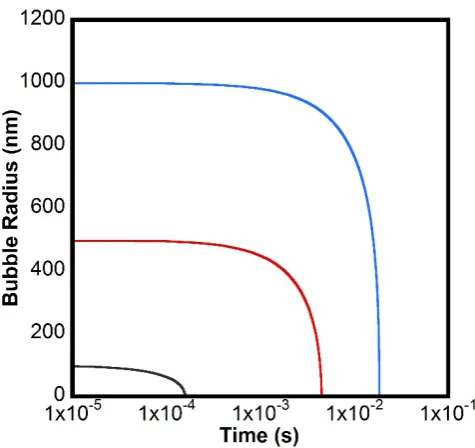
The change in size for a bubble with an initial radius of 100 nm, 500 nm, and 1000 nm were

calculated using Equation1_{1.11 (see Figure 1-3). Here the calculation was done in small time}

steps and the Laplace pressure and Cs was recalculated at each step to account for the effect of

the shrinking radius, allowing for accurate calculations for small bubbles. As shown, the theory

predicts that small bubbles will rapidly shrink and disappear in saturated solutions. For example, the lifetime of a bubble of initial radius of 1000 nm is predicted by the Epstein and Plesset theory to be less than 0.02 s. Such bubbles would in most cases dissolve and disappear

(27)

[image:27.595.74.312.71.295.2]

Figure 1-3 Calculated nanobubble radius versus time using the Epstein and Plesset theory1 for a nitrogen filled nanobubble of initial radius 1000 nm (blue), 500 nm (red), and 100 nm (black) in a solution that is saturated with dissolved nitrogen gas. For this calculation, equation 1.11 was implemented iteratively to take account of the increasing Laplace

pressure with decreasing size. The parameters used in this calculation are T = 300 K, γ =

0.072 Jm-2_,_D_{= 2.0 × 10}-9_m2 _s-1_,_C

(28)

1.3.2.2 The lifetime of bubbles

In 1997, Ljunggren and Eriksson developed a theory to specifically calculate the Lifetime of

bulk nanobubbles2_{. This work was reported in direct response to reports of the existence of}

surface nanobubbles65_{. Their calculation was in agreement with Epstein and Plesset’s theory,}

and they stated that “bubbles of colloidal size in water have a short lifetime”. Their expression

for the lifetime for a bubble with initial radius r0 is given in equation 1.12:

𝑎𝑎 =_{3𝑅𝑅𝑅𝑅𝐷𝐷}𝐾𝐾𝐻𝐻𝑟𝑟02 (1.12)

where t is the lifetime of the bubble, KH is Henry’s law constant, R is the ideal gas constant, T

is the temperature, and D is the diffusion constant.

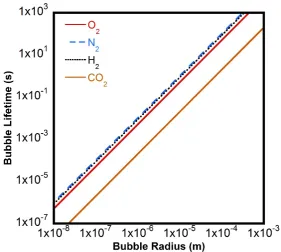
Figure 1-4 shows the expected lifetime for a gas bubble as a function of its initial radius2_using

the Ljunggren and Eriksson model (equation 1.12). It is clearly demonstrated that such a nanoscale bubble will dissolve very quickly. The calculation in Figure 1-4 also considers the

(29)

[image:29.595.72.354.76.328.2]

Figure 1-4: Expected lifetime for a bubble in water as a function of the initial radius and

gas type using the Ljunggren and Eriksson model (equation 1.12)2,64_{. The parameters used}

in this calculation are KH (O2) = 7.7 ×104 J mole-1, KH (N2) = 15.6 ×104 J mole-1, KH (H2) = 13 ×104_{J mole}-1_,_K_H_(CO₂_{) = 0.3 ×10}4_{J mole}-1_{, D = 2.0 × 10}-9_m2 _s-1_{, and T = 298 K.}

The findings from Epstein and Plesset and Ljunggren and Eriksson have had a profound influence on nanobubble research, as it has led to reports of long-lived nanobubbles being

(30)

1.4 Nanobubbles Research

Two types of nanobubbles are reported in the literature. The term bulk nanobubbles is used to

describe gas filled bubbles in solution that have a diameter less than 1000 nm. Ultrafine bubbles

is an equivalent term that is also used in the literature. The term surface nanobubbles is used to

describe gaseous domains attached to surfaces. The height of surface nanobubbles is generally more than 10 nm and less than 100 nm. The radius of the contact line (three-phase line) is

generally between 50 and 500 nm. The existence of stable surface nanobubbles has now been established66,67_{, although the origin of their stability is still debated}68–74_{. However, the focus of} this study is bulk nanobubbles and the relationship, if any, between surface and bulk

nanobubbles has not be elucidated.

1.4.1 Bulk Nanobubbles

1.4.1.1 Early Reports of Bulk Nanobubbles

Perhaps, the first report of bulk nanobubbles was in 1962 by Sette and Wanderlingh75_{. They}

demonstrated that high-energy neutrons present in cosmic rays or introduced artificially reduced the sound energy required to initiate cavitation of bulk water. They argued that oxygen recoil nuclei deposit energy that results in the formation of cavitation nuclei which are stabilized

by contaminants. Further, they showed that by shielding water from neutrons, the cavitation threshold energy increased over a period of ~5 hours, indicating that the microcavities persisted

for at least this long. Later, Hemmingsen76_{studied cavitation in solutions that were}

supersaturated with gas and found that the supersaturation threshold for cavitation could be increased by prior application of extremely high pressures. This was attributed to the removal

(31)

the cavities76_{. During the 1990s, Bunkin}_{et al}_.77–79_{reported the existence of stable microbubbles}

in dilute solutions of electrolytes. These microbubbles were thought to be stabilized by repulsive interactions between ions adsorbed to the interface and provide nuclei for optical

cavitation. More details about this mechanism is given in §1.4.1.5.

1.4.1.2 Production and Characterisation of Bulk Nanobubbles

There are several publications on long-lived bulk nanobubbles that have been generated through several techniques. All of these methods rely on the inducement of supersaturation, which could

nucleate nanobubbles. These techniques include ultrasonication, electrolysis, solvent exchange, temperature changes and mechanical means.

1.4.1.2.1 Ultrasonication

Kim et al. in 200043_{, reported the generation of bulk nanoparticles by sonication (42 kHz, 70W}

) in the presence of a palladium coated surface, directly in a cuvette placed in a dynamic light scattering (DLS) apparatus. In purified water they produced a bimodal distribution of

nanoparticles with peaks around 80 nm and 350 nm. Particles created at pH 3 were slightly larger than particles created at pH 12. The particles were designated to be nanobubbles. The measured zeta potential for the nanoparticles was consistent with reports of the zeta potential

measured on larger bubbles80_{. The nanoparticles were stable for at least 60 minutes. In this}

(32)

this manner. Ultrasonication has also been used recently by Mo et al. 84_{to study the generation}

of bulk nanobubbles84_{. They used nanoparticle tracking analysis to compare the concentration}

of nanoparticles in i) pure water, ii) water after 1 min ultrasonication and iii) degassed water

after ultrasonication. They concluded that the nanoparticles generated by ultrasonication were gas-filled nanobubbles because the concentration of nanoparticles in the water after ultrasonication was higher than the concentration of the nanoparticles in the other two samples.

The concentration of the produced nanoparticles was measured to be ~ 7×107 _{particles/ml,}

which corresponds to less than 5 particles/frame. However, a lower concentration of the

particles upon degassing is not necessarily direct evidence of nanobubbles as volatile oil

droplets respond to vacuum in a similar way to bubbles85_.

1.4.1.2.2 Electrolysis of Aqueous Electrolyte Solutions

Electrolysis of water evolves gas and supersaturates the solution with hydrogen gas at the

cathode and oxygen gas at the anode. Between 2001 and 2009, Kikuchi et al. studied the

generation of nanobubbles by electrolysis46,47,86–88_{. In the cathodic solution, particles 10 - 600}

nm in diameter were detected by Dynamic Light Scattering (DLS) and shown to be stable for

at least four hours87_{. In the anodic solution, particles 30 nm in diameter were produced by}

electrolysis and measured over three days, after which they had increased in size to 250 nm.

After five days, particles were no longer detected47_{. According to the authors, the particles in}

the anodic and cathodic solutions were oxygen and hydrogen nanobubbles, respectively. This

work also showed that oxygen contained within the nanoparticles was not detected when using a standard dissolved oxygen meter or the Winkler oxygen titration method. However, if the pH of the solution was reduced by the addition of acid, the Winkler method detected an increase in

oxygen concentration, which was attributed to the oxygen liberated from the nanobubbles. In

recent work, Postnikov et al. 89_{used electrolysis to produce and control the size of the}

(33)

were nanobubbles. The lifetime for these nanoparticles was found to be 15 minutes, which was

less than the lifetime for the nanoparticles reported by Kikuchi47,87_{. However, a lifetime of 15}

minutes is still much longer than the lifetime expected from the Epstein and Plesset theory1_.

1.4.1.2.3 Mechanical Generation

Another common method that is reported to produce bulk nanobubbles is based on mechanical

means48–51,90–93_{. These methods use pressure-cycling techniques where the solution is subject}

to an increase in pressure to increase the solubility of gas, followed by a reduction in pressure which is expected to result in the formation of bubbles. Many of these techniques also employ gas injection. An example is the study by Ushikubo and his group, who used oxygen gas to

produce what they designated to be nanobubble solutions49_{. The average size of the}

nanoparticles produced was determined to be 137 nm, measured by dynamic light scattering (DLS). The generated nanoparticles were shown to be stable for days, and they attributed their

stability to the electric charge at the interface, as the zeta potential was measured to be in the range of -45 mV to -34 mV. In a recent study, Wang et al. reported that N2, O2 and CO2

nanobubbles could be produced and maintained stability for at least 24 hours90_{. In this study,}

they were able to adjust the size of the nanoparticles by adjusting the periodic pressure time interval during generation. They found that the size of the nanoparticles decreased with an

(34)

solvents studied, except hexane. They claimed that nanobubbles could be generated

mechanically in a range of organic solvents.

1.4.1.2.4 Solvent Exchange

Solvent exchange was first reported in 2000 as a convenient method for producing surface

nanobubbles94_{. The process was as follows: the hydrophobic surface was initially immersed in}

a water-miscible solvent (e.g. ethanol), and then the ethanol was slowly displaced by water.

Common atmospheric gases, such as nitrogen and oxygen, have lower solubility in the ethanol-water mixture than prior to mixing. Hence during solvent exchange, supersaturation is occurred

and gas precipitates onto the surface, leading to the formation of surface nanobubbles. An et al

.95_{showed that the saturation level could reach up to 311% upon mixing ethanol and water.}

This method has been commonly employed to produce surface nanobubbles. Several groups

have used solvent mixing to generate bulk nanobubbles44,96–100_{. In a series of publications in}

2007, Jin et al. 44,96,97_{examined aqueous solutions of tetrahydrofuran, ethanol, urea, sugars,}

surfactants and α-cyclodextrin using dynamic laser light scattering. These measurements, as

well as those of other researchers, revealed a ‘slow mode’ which corresponds to structures ~

100 nm in diameter. It was found that the slow mode could not be removed by simple filtration through a 20 nm pore-sized filter, but it was gradually removed by numerous repeated

filtrations, regardless of the type of solute present. Moreover, the slow mode was restored by the injection of particle-free air. They concluded that the slow mode was a signature of

nanobubbles that were stabilized by surface active organic molecules. However, Habich et al.41

and Sedlak et al.101_{performed similar experiments using degassed solutions and found that the}

level of light scattering remained significant. They attributed the scattering to contaminants

(35)

generated nanoparticles using ethanol-water mixing. They investigated the effect of the ratio of

ethanol to water on the size and concentration of nanoparticles produced as measured by nanoparticle tracking analysis. The maximum concentration of nanoparticles was obtained at

8.3% v/v ethanol solution. Contrary to the works of Habich et al. 41_{, they concluded that these}

nanoparticles were gas-filled nanobubbles based on their observation of a reduction in the concentration of nanoparticles when mixing degassed solvents.

1.4.1.2.5 Increasing the Temperature of Solution

Najafi et al. 45_{produced what was claimed to be nanobubbles in a closed cuvette for zeta}

potential measurement by increasing the temperature. This reduced the solubility of dissolved

gases and precipitated nanobubbles, which had a mean size of 290 nm. The measured zeta potentials were consistent with those measured for larger bubbles. Before the temperature change, no scattering was detected. Note a temperature increase leads to an increase in solubility

for most materials, particularly candidate contaminants such as hydrocarbons, further supporting their assertion that the nanoparticles were nanobubbles.

1.4.1.3 Additional Methods used to Characterise Bulk Nanobubbles

The above experiments utilized standard techniques for nanoparticle characterization, such as

(36)

scanning electron microscopy, revealing a population of nanoparticles. The images are

reproduced in Figure 1-5.

Figure 1-5. Panel A: Scanning electron microscopy image of rapid cryogenic freezing fracture of a solution of nanoparticles that was assigned to be nitrogen nanobubbles with a diameter of ~ 100 nm. Panel B: A higher magnification image of a single nanoparticle. Images are reprinted from [K. Ohgaki, N.Q. Khanh, Y. Joden, A. Tsuji, T. Nakagawa, Physicochemical approach to nanobubble solutions, Chem. Eng. Sci. 65 (2010) 1296–1300. doi:10.1016/j.ces.2009.10.003.] Copyright (2019) with the permission of Elsevier.

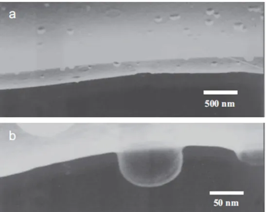
In a complementary study, Uchida et al. 50_{produced nanoparticle solutions by gas injection of}

ultrapure oxygen. Rapid cryogenic freezing was then used to prepare replicas of the surface of

a fractured water droplet, and the resulting replica was imaged by transmission electron microscopy. Nanoparticles ~ 100 nm in size were revealed (see Figure 1-6). In later work, they showed that nanoparticles produced in the same manner increased in size from ~ 400 nm to ~

750 nm over a period of a week when stored in a sealed bottle102_{. Cryo-EM has been employed}

to directly image bulk nanobubbles embedded in amorphous ice that was produced by a

nitrogen-evolving chemical reaction103_{. A concern is that sample freezing leads to unavoidable}

[image:36.595.75.349.135.353.2]

(37)

freezing. Countering this is the extensive use of this technique in biological imaging and the

[image:37.595.75.224.156.456.2]

general acceptance of the conclusion that rapid freezing does not generally produce artefacts of this nature.

Figure 1-6. Replica transmission electron microscopy images showing spherical objects

thought to be O2 filled nanobubbles with a diameter of ~ 500 nm (a) or 200 nm (b). Panel c

(38)

registered a significantly lower refractive index than the surrounding medium. Significantly,

unlike most other studies of bulk nanobubbles, the solution was not supersaturated with dissolved gas.

Kobayashi et al. were the first to utilize the resonant mass measurement technique in

characterizing bulk nanobubbles51_{. An instrument called the Archimedes was used to detect the}

mass density relative to the solvent of individual nanoparticles as they passed one by one

through a microresonator105_{. (The details of this method are reported in §2.3). Measurements}

on nanoparticles generated by pressure cycling revealed a population of nanoparticles with positively buoyant mass, indicating that they were less dense than the solvent. However, light oil droplets also have a density less than water, and therefore this alone is not sufficient evidence

to demonstrate that they are gas filled bubbles.

Oh et al.92_{adapted a technique that was previously used on surface nanobubles}66_{to investigate} the presence of bulk nanobubbles. The infrared spectra of what they attributed to be bulk

nanobubbles exhibited a rotational fine structure that was consistent with CO2 molecules in

their gaseous state, whereas their control, CO2-saturated water exhibited a single peak at 2343

cm-1_{, indicating the presence of dissolved CO}_2._{However, there was no direct evidence that the}

spectra were obtained from the nanobubbles in the bulk of the solution as opposed to surface

nanobubbles or larger bubbles. Nirmalkar et al. recently used a freeze-thaw technique as a

method for differentiating nanobubbles from other nanoparticles62,106,107_{. In their study, they}

generated nanoparticles that were stable for up to a year, using ultrasound cavitation. They concluded that these were nanobubbles, as these nanoparticles disappeared after the freeze-thaw

process. Furthermore, they showed that the addition of surfactant (i.e., SDS) to the

nnaoparticles62_{before the freezing process stabilized the nanoparticles, which prevented them}

(39)

nanoparticles or cream out of the solution if they were oil droplets. Significantly they did not

investigate the effect of the freeze-thaw treatment on a known nanoparticle sample.

In contrast to the conclusions of all the above studies, Leroy et al.42_{have examined solutions}

treated with a bubble generator for evidence of bulk nanobubbles using ultrasound and found no evidence of bulk nanobubbles. This technique is of interest, as it sensitive to the presence of

gas. However, this technique as applied is not sensitive enough to detect the typical reported

concentrations of nanobubbles (108_/mL).

1.4.1.4 Evidence of Bulk Nanobubbles

The above experiments are correctly criticized for a lack of direct evidence that the

nanoparticles being observed actually consist of gas. However, a number of experiments provide more direct evidence of long-lived gas filled bulk nanobubbles. Possibly the earliest

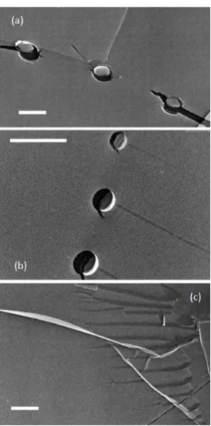
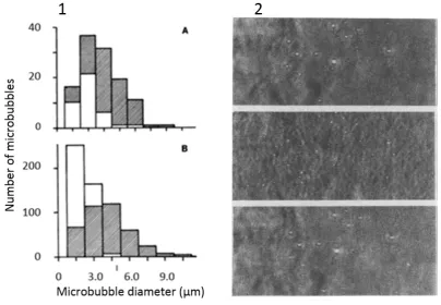
direct evidence of bulk nanobubbles with diameters less than a micron was reported by Johnson

and Cooke in 1981108_{. They reported that bubbles produced by shear in seawater were observed}

to be stable for long periods (>22 hours) due to the formation of surface films formed from

naturally present surfactants. They demonstrated that such encased bubbles were gas-filled, as they expanded when put under tension (negative pressure) and contracted under an applied

pressure (see panel 1 in Figure 1-7), and some could even be destroyed by application of

(40)

gelatine. Similar to the work of Johnson and Cooke108_{, they showed that the observed objects}

were gas-filled bubbles that expanded and contracted under the depressurizing and pressurizing process (see panel 2 in Figure 1-7). They pointed out the possibility of forming nanobubbles

(41)

Figure 1-7. Early measurements on the effect of external pressure on the size of small

bubbles108,112_{. Panel 1A shows the distribution of bubbles in seawater (shaded region)}

[image:41.595.74.479.78.358.2]

(42)

The strongest evidence for the existence of long-lived nanobubbles comes from their contrast

in ultrasound imaging9,113,114_{. Here, bubbles are used to enhance the echo ultrasound signal to}

improve the contrast during ultrasound imaging. In 2004, Oeffinger and Wheatley employed

surfactant stabilized nanobubbles as ultrasound contrast agents9_{. The initial population of}

surfactant stabilized bubbles was produced by the sonication of a perfluorocarbon gas. This produced a population of bubbles with a mean diameter of > 1 micron. This sample was then

centrifuged to promote creaming of the larger bubbles. In doing so, the mean diameter of the dispersion was reduced to ~ 400 nm. The evidence that these objects are indeed nanobubbles is

two-fold. Firstly, they were demonstrably less dense than water, as the larger particles creamed more effectively during centrifugation. Secondly, these nanoparticles provide an ultrasound enhancement compared to a control buffer without the nanoparticles. This is consistent with the

particles being gas-filled nanobubbles as opposed to oil droplets. In recent work, Hernandez et

al. produced smaller lipid-stabilized nanobubbles with a mean diameter of 290 nm115_{. Resonant}

mass measurement was employed in their measurement and showed that these bubbles were less dense than their solvent. The ultrasound contrast enhancement coming from these bubbles was significant, and it was higher than the signal of commercial microbubbles. Additionally,

they showed that the number of these nanobubbles decreased significantly after exposing the nanobubbles to high-power ultrasound indicating destruction of the bubbles.

It is notable that all the direct evidence of bulk nanobubbles above is associated with bubbles that were coated with insoluble material, which likely contributed to their stability68_{. In contrast,}

(43)

1.4.1.5 Explanations for the Stability of Unarmoured Bulk Nanobubbles

Although the existence of unarmoured nanobubbles is not yet widely accepted, a number of

explanations have been proposed to explain their stability. In some cases, the solution is highly supersaturated, and this will extend their lifetime. If the solution is saturated such that it is in equilibrium with the nanobubble, the predicted bubble lifetime is infinite. However, a very

small deviation from the equilibrium condition dramatically influences the stability. Such that a deviation of only 0.0001% below the saturation level would see the nanobubble dissolve in

two seconds (see Figure 1-8). Similarly a fluctuation in size of a nanobubble that is in the equilibrium condition would see the nanobubble rapidly shrink or grow and leave solution due to buoyancy. Thus, the stability of nanobubbles is never likely to be maintained for any

[image:43.595.75.305.391.616.2]

(44)

required for equilbrium leads to rapid dissolution of the bubble. The parameters used in this calculation are T = 300 K, γ = 0.072 J m-2_,_D_{= 2.0 × 10}-9_m2 _s-1_,_C

sat = 0.6379 moles m-3, and ρ1 atm= 40.6921 moles m-3.

The effect of extremely high concentrations of nanobubbles has also been considered. Under

these circumstances, the diffusion of gas out of a nanobubble is slowed by the effective increase

in dissolved gas concentration due to the surrounding bubbles116_{. This is likely only to be}

significant at extremely high volume fractions. In the work of Johnson and Cooke108_{, the}

formation of a skin of contaminant molecules was clearly implicated in the stability of the bubbles they observed. However, in other nanobubble preparations, the level of contamination

would be much lower, so this is unlikely to be a universal stabilizing mechanism. Bunkin78

proposed that ions at the air-water interface repel each other, effectively reducing the surface tension. However, this implies that the air-water interface cannot charge regulate and that the

concentration of ions at the interface would not be determined by the chemical potential set by the concentration in the bulk. Thus this proposed mechanism violates basic thermodynamics.

Despite the obvious problems with this mechanism a recent work by Nirmalkar et al. 106_invoked

the same mechanism.

Yasui et al. 117_adapted_{the equilibrium model proposed by Brenner and Lohse}69_{to explain the}

stability of surface nanobubbles. In this case, solid particles adsorbed to the nanobubble surface are thought to provide a reservoir of gas, as the substrate does in the dynamic equilibrium

model. This model has already been abandoned for surface nanobubbles, in part because it requires a constant input of energy, lest it violate the second law of thermodynamics. The

adaptation here requires that a reasonable fraction of the nanobubble surfaces are covered in hydrophobic particles, which is not supported by the experimental evidence. Nor does this modification overcome the fundamental violation of thermodynamics in the dynamic

(45)

1.4.1.6 Use and Potential Applications of Bulk Nanobubbles

Despite the lack of direct evidence for the existence of bulk nanobubbles, the level of industry

activity and interest in the field is rapidly increasing. This is reflected in the growing membership of the Fine Bubble Industries Association (FBIA) and the rising number of patents in the area. Below is a brief summary of the currently reported and potential applications of

bulk nanobubbles. Many of these applications depend on the nanobubbles being present in solution for extended periods of time.

The motion of nanobubbles in solution is influenced by the terminal rise velocity and Brownian

velocity. The terminal rise velocity of a spherical bubble of a radius r due to buoyancy 𝑈𝑈𝑇𝑇, is

dependent on the boundary condition, and for a no-slip boundary condition, is given by:

𝑈𝑈𝑇𝑇 = 2𝑟𝑟 2_{Δ𝜌𝜌𝜌𝜌}

9𝜂𝜂 (1.13)

where Δρ is the difference in density between the bubble and the solution, g is the acceleration

due to gravity, and η is the viscosity of the liquid. If a slip boundary condition is employed,

then the terminal velocity is 1.5 UT, though studies show that a no-slip boundary condition is

appropriate in nearly all cases, due to minute amounts of contamination118,119_{. The calculated}

no-slip terminal rise velocity for a nanobubble of radius 50 nm is 6.12 nm s-1_{and for a}

(46)

where kB is the Boltzmann constant, T is the temperature, η is the viscosity, and r is the particle

radius.

For a nanobubble of a radius 50 nm and 500 nm, the Brownian velocities are 3131 nm s-1_and

990 nm s-1_{, respectively. Comparison of these two values to the rise velocity shows that the}

Brownian motion dominates the behaviour of the nanobubbles and will act to mix them in solution and oppose the effect of buoyancy.

A number of applications make use of this, particularly those that require the oxygenation of

water, as smaller bubbles have longer residence times, and therefore have more time to deliver gas into solution and a larger surface area for a given volume. Moreover, smaller bubbles have

higher Laplace pressures and consequently increase the solution saturation concentration of the gas surrounding a bubble. This could potentially have a significant effect if large numbers of nanobubbles were produced. The various applications for bulk nanobubbles are discussed in

detail below.

1.4.1.6.1 Biological and Medical Applications

Bulk nanobubbles are increasingly finding biological and medical applications. Bubbles are

effective ultrasound contrast agents, since their acoustic response is very different from that of

tissues and fluids121_{. Nanobubbles used for ultrasound imaging have been used in several}

studies3–8,115_{, due to their ability to easily pass through the vasculature. For instance, Fan}_et

al.122_{compared the echogenic properties, both}_{in vitro}_and_{in vivo}_{, of lipid-coated nanobubbles}

with an average size of 435.2 ± 60.5 nm with a commercial standard (SonoVue®_microbubble

contrast agent), and found that a higher contrast was achieved using nanobubbles. A similar

study performed by Yin et al. 8_{showed that lipid coated (armoured) nanobubbles with a mean}

diameter of 436.8 ± 5.7 nm provided a greater contrast enhancement than microbubbles. The ultrasound images from this study are shown in Figure 1-9. Further, they showed that the

(47)

‘multicoloured’ nanobubbles for disease diagnostic applications by encapsulating three types

of fluorophores into the lipid-coating of nanobubbles for a combination of fluorescence resonance energy transfer (FRET) and ultrasound imaging. Variations in the ratios of three dyes

caused the nanobubbles to register multicolour images under single wavelength excitation, allowing the differentiation of the two tumours.. Further, they showed that two tumour regions exhibited comparable fluorescence signals when triple-dye-doped nanobubbles and

dual-dye-doped nanobubbles were injected. This was demonstrated in a tumour on the left hand side of a mouse following the injection of dual-dye-doped nanobubbles, which exhibited a stronger

signal compared to a tumour on the right hand side following the injection of triple-dye-doped nanobubbles when the fluorescence signal was 670 nm. The weak and strong florescence signals coming from these two tumours were flipped when they performed the FRET

fluorescence imaging using the same nanobubbles but with a fluorescence signal of 790 nm. They hypothesized that this technique could be further developed to distinguish different tissues

in a complex clinical diagnosis. Another great area of interest for nanobubbles is their potential

use in therapeutic drug delivery6,9–11_{. They can be fabricated for drug delivery purposes by}

incorporating lipids with head-groups that specifically bind the drug124,125_{, which can be}

released when the nanobubbles are irradiated with high levels of ultrasound energy. Candidate nanobubbles or related entities have also been implicated in an oxygenated medical saline for

(48)

Figure 1-9. Representative set of comparison tumour images before and after injecting nanobubbles (A), and microbubbles (B) into tumour-carrying mice at different times: 0.0, 0.5, 1,5, 10.0 and 15.0 minutes. Images are republished from [T. Yin, P. Wang, R. Zheng, B. Zheng, D. Cheng, X. Zhang, X. Shuai, Nanobubbles for enhanced ultrasound imaging of tumors., Int. J. Nanomedicine. 7 (2012) 895–904. doi:10.2147/ijn.s28830] Copyright (2019) with the permission of Dove Medical Press Ltd.

1.4.1.6.2 Plant Growth and Seed Germination

Candidate nanobubbles are reported to have considerable impact on plant growth and seed

germination30–37_{. Ebina}_{et al}_{. have claimed that water infused with oxygen nanobubbles, less}

(49)

growth of plants exposed to oxygen nanobubbles with controls are shown in Figure 1-10. This

effect was further investigated through the use of four types of gasses (i.e., air, nitrogen, oxygen

and carbon dioxide) on seed germination and plant growth by Khaled et al.30_{. All types of}

nanobubbles except the air nanobubbles were reported to enhance plant growth, but only nitrogen nanobubbles showed a significant effect on the seed germination. It is odd that the air nanobubbles did not have an effect on the growth, whereas nitrogen and oxygen nanobubbles

showed an effect. This casts doubt on this research. A recent two-year field experiment

conducted by Zhou et al.35_{showed that candidate microbubble/nanobubble dispersions had a}

positive impact on maize roots, although they demonstrated that the effect was also associated with the concentration of dissolved oxygen, where the optimum level was at 20 mg/L. Nanobubbles have also been reported to disrupt water transport, due to hydraulic failure in the

(50)

Figure 1-10: Comparison of the growth of plants cultured with normal water and candidate air-nanobubble dispersions. Images are republished from [K. Ebina, K. Shi, M. Hirao, J. Hashimoto, Y. Kawato, S. Kaneshiro, T. Morimoto, K. Koizumi, H. Yoshikawa, Oxygen and air nanobubble water solution promote the growth of plants, fishes, and mice., PLoS One. 8 (2013) e65339. doi:10.1371/journal.pone.0065339] Copyright (2019) with the permission of Plos One.

1.4.1.6.3 Water Treatment

The use of nanobubble dispersions for oxygenation is also being applied in the bioremediation

of groundwater pollution15_{and in water treatment}12–17_{. Ushida}_{et al.}50_{observed that}

nanobubbles collected impurities on their surfaces and hence they could be used to capture and remove these impurities. They argued that the effectiveness of this technique would depend on

(51)

efficient method for remediation of wastewater contaminated with organic matter. They argued

that the effectiveness of nanobubble water treatment was pH sensitive, with the highest

efficiency for ozone nanobubbles being at pH 5. A recent study by Kyzas et al. 17_investigated

the effects of nanobubbles on the adsorption of lead ions to activated carbon. They found that the main effect was not on the adsorption capacity, but on the adsorption rate, claiming an acceleration of the adsorption process by 366%.

1.4.1.6.4 Froth Flotation

The use of nanobubbles to separate hydrophobic solid particles in mineral flotation has been

extensively investigated18–29_{. It is worth noting here that flotation studies have been conducted}

using a combination of what has been reported as nanobubbles and larger bubbles; utilising nanobubbles by itself in flotation is inefficient because of their low buoyancy. The suggested mechanism is that nanobubbles adsorb onto the surface of hydrophobic particles, thus

promoting their attachment to larger bubbles by acting as a bridge between the particles and the

larger bubbles27_{. In a series of publications, Maoming}_{et al}_{. suggested that the presence of}

nanobubbles with larger bubbles can provide the optimum conditions for the flotation of

hydrophobic particles20,21,24–29_{. In their studies, they used hydrodynamic cavitation to produce}

candidate nanobubble dispersions and conventional-sized bubbles, and examined their effect

(52)

advantageous and would eliminate the need to remove the flocculant for downstream

processing.

1.4.1.6.5 Cleaning

Bulk nanobubbles are being claimed for cleaning applications, as the dispersion of nanobubbles

presents a significant surface area of high interfacial tension, which can attract contaminants due to favourable energetics and thereby prevent their deposition onto surfaces. Candidate

nanobubbles have been reported to effectively clean membrane-fouled surfaces136_{. They have}

also been reported to be used in cleaning textiles137_{. Ushida}_{et al.}_{claimed that water containing} what was assigned to be nanobubbles exhibited a higher washing rate for textiles soiled with

hydrophobic organics by 5 % compared to control water not treated with nanobubbles137_{. The}

absence of added surfactants means that chemical residues are avoided and the cleaning process is more environmentally friendly.

1.4.1.6.6 Hydrogen Fuels

A high profile claim made by Oh et al.39,40_{suggested that hydrogen nanobubbles can be}

introduced as an energy source for improving engine performance39,40_{. Oh}_{et al.}_{argued that}

gasoline fuels containing what was assigned to be hydrogen nanobubbles were more efficient than conventional gasoline fuel39_{. In another study}40_{, they claim that the change in the chemical}

composition of gasoline in a “hydrogen nanobubbles gasoline sample” was measured using chromatography/mass spectrometry, could be the reason for the improvement in efficiency.

1.4.1.7 Summary

Reports that armoured nanobubbles are gas filled are supported by their response to ultrasound.

(53)

led to a proliferation of claims many of which are unsupported. Therefore, it is important to

systematically examine the existence of bulk nanobubbles. To this end, the development of an easily conducted test or tests that can consistently and reliably differentiate nanobubbles from

(54)

1.5 Aims and Structure of the Thesis

This study aims to

1. Develop a protocol that can be applied to a dispersion of unknown nanoparticles to

determine with confidence whether they are gas filled bubbles or otherwise.

2. Investigate methods that have been reported to produce long-lived bulk nanobubbles.

This knowledge will be used to address fundamental issues in the field, such as understanding what conditions (if any exist) are required for nanobubbles to be long lived.

The following hypotheses will be tested in this study

• The pressure response of nanobubbles can be used to differentiate them from other

nanoparticles, even when the nanobubbles are armoured with a shell of insoluble lipid.

• The density of nanoparticles can be determined using the resonant mass measurement

method.

• Long-lived bulk nanobubbles can be generated by mechanical means.

• The mixing of ethanol and water produces stable long-lived bulk nanobubbles.

• Supersaturation obtained by a chemical reaction produces long-lived nanosized bubbles

(55)

1.5.1 Outline

The remainder of this thesis is organised as follows

Chapter 2 describes the main characterization techniques used in this study, including dynamic

light scattering, nanoparticle tracking analysis, and resonant mass measurement.

In Chapter 3, the methods developed to distinguish bulk nanobubbles from other nanoparticles are explained in detail. This includes size measurement under the application of external

pressure and the determination of nanoparticle density. These methods were applied to armoured nanobubbles that are usually used in ultrasound imaging. The results of these experiments are discussed in detail. These techniques have been applied in chapters 4-6.

Chapter 4 investigates the existence of long-lived bulk nanobubbles produced using two

different devices that are designed to produce bulk nanobubble solutions by mechanical means.

In Chapter 5, a simple method for generating nanoparticles by mixing ethanol and water is presented. The constitution of these particles whether they are gas filled or otherwise is determined and how the nanoparticles are formed is explained.

In Chapter 6 the hypothesis that nanobubbles can be generated using a gas evolving chemical

(56)

Chapter 2 Experimental Procedures

A range of methods were employed in this study to provide fundamental information about the nanoparticles such as their average size, concentration, buoyancy, and stability. The techniques

described here are shared across most of the research described in later chapters. Techniques that are applied exclusively to a specific portion of the research are reported later in the experimental methods section of the chapter describing that research.

The size distributions of nanoparticles in this study were measured using light scattering

methods such as dynamic light scattering (DLS) and nanoparticle tracking analysis (NTA). Resonant mass measurement (RMM) was used to measure the size and buoyant mass of nanoparticles in solution. This chapter provide an overview of each technique including a brief

discussion of their capabilities and limitations.

2.1 Dynamic light scattering

In this study, a Zetasizer Nano ZS (Malvern) employing a 633 nm He−Ne laser at a scattering

angle of 173° was used to measure the size of particles in solution using dynamic light scattering (DLS).

Dynamic light scattering (DLS), which is also known as photon correlation spectroscopy (PCS), is used to measure the hydrodynamic size of dispersed particles. If a laser light is shone onto a

group of stationary particles, they will interact with the electromagnetic radiation and scatter light in different directions. If a detector is placed at a specific angle from the sample, the

(57)

due to the constructive and destructive interference of the scattered waves from the particles138_.

In reality, suspended particles in solutions are never stationary, rather they move randomly due to Brownian motion. This leads to fluctuating patterns over time. In DLS, the fluctuation in the

net intensity of the scattered light is quantified using an autocorrelation function. Small particles that move quickly due to Brownian motion result in a fast decay in the autocorrelation function. In contrast, large particles cause a slow decay in the autocorrelation function. An example of

raw correlation data is given in Figure 2-1A below.

For suspended monodisperse particles in solution undergoing Brownian motion, the exponential decay for the correlation function G(τ) withdelay time τ is expressed as138

𝐺𝐺(𝜏𝜏) =𝐴𝐴𝑒𝑒−𝐷𝐷𝑞𝑞2_𝜏𝜏

+𝐵𝐵 (2.1)

Where A is the amplitude of the correlation function, which is the intercept the correlation decay, D is translational diffusion coefficient of dispersed particles, B is the baseline, and q is

the magnitude of the scattering vector which is related to the angle θ by

𝑞𝑞=4𝜋𝜋𝑛𝑛_𝜆𝜆 𝐷𝐷sin𝜃𝜃₂ (2.2)

where nDis the refractive index of the solvent

DLS uses the Stokes-Einstein law to extract the average size of nanoparticles from the diffusion

(58)

where kB is the Boltzmann constant, T is the temperature, η is the viscosity, r is the particle

radius, and c is 4 for a slip boundary condition and 6 for a no-slip boundary condition. If the

wrong boundary condition is used, the error in the measured size may be substantial; a particle with a slip boundary condition analysed using a no-slip boundary condition would have its size

underestimated by one-third. Generally, a no-slip condition is assumed in equation 2.3. This assumption is accurate for solid particles and liquid droplets. For nanobubbles, it is possible that a slip boundary condition should be used as the gas-liquid interface is often treated with a

slip boundary condition. However, analysis of the rise velocity of bubbles in purified water shows that only when water has undergone extreme purification measures is a slip boundary

condition evident for a bubble that is more than a few seconds old 118,119_{. Therefore, it is}

appropriate to use the no-slip boundary condition here, even for nanobubble samples (i.e., c =

6 in equation 2.3).

DLS provides three types of distributions: intensity, volume, and number distribution. The

intensity distribution reflects the raw distribution obtained by the DLS technique. It is worth noting that the size measurements based on intensity distribution are more sensitive to large particles than to small particles. This is due to the proportional relationship between the

intensity of scattered light and the sixth power of the diameter of the detected particle according

to the Rayleigh approximation139_.

𝐼𝐼 ≈ 𝑑𝑑6 _(2.4)

These limitations must be borne in mind when using the results from the Zetasizer. The other two distributions are useful but less accurate as they are derived from the intensity

measurements using Mie theory140,141_{. The volume distribution shows the total volume of}

particles in different size bins, whereas the number distribution shows the number of particles

(59)

absorption. Thus, the volume and number distribution can only be used if the optical properties

of the material and solvent are known.

DLS is suitable for measuring monodispersed samples. It measures particles ranging from 0.3 nm to 10 µm. It does not require a large sample volume or long periods of time for sample preparation. However, an appropriate sample concentration is needed to meet the quality criteria

for measurement, where the minimum and maximum concentrations are 0.1 mg/ml. and 40 % weight/volume, respectively.

A typical DLS size measurement for a standard nanoparticle is shown in Figure 2-1 . The

measurements were made with automatic attenuation at a position of 4.65 mm from the cuvette wall and analysed using the Malvern Zetasizer software version 7.1.