Parallel Deterministic Annealing Clustering and its Application to LC MS Data Analysis

Parallel Deterministic Annealing Clustering and its Application to LC-MS Data

Analysis

Geoffrey Fox

School of Informatics and Computing Indiana University

Bloomington IN USA gcf@indiana.edu

D. R. Mani

Proteomics and Biomarker Discovery The Broad Institute of MIT and Harvard,

Cambridge, MA USA manidr@broad.mit.edu

Saumyadipta Pyne

CR Rao Advanced Institute of Mathematics, Statistics and Computer Science, Hyderabad, India.

spyne@crraoaimscs.org

Abstract—We present a scalable parallel deterministic annealing formalism for clustering with cutoffs and position dependent variances. We apply it to the “peak matching" problem of the precise identification of the common LC-MS peaks across a cohort of multiple biological samples in proteomic biomarker discovery. We find reliably and automatically tens of thousands of clusters starting with a single one that is split recursively as distance resolution is sharpened. We parallelize the algorithm and compare unconstrained and trimmed clusters using data from a human tuberculosis cohort.

Keywords – deterministic annealing, clustering, LC-MS, proteomics, performance, parallel algorithms

I. INTRODUCTION

Big data emerging from different aspects of health and “omics” profiling of biological samples in the quest to understand disease, require scalable and robust analysis. Strategies for early recognition of outbreak of an infectious disease and rapid initiation of infection control are of key importance in maintaining public health and security. International grids connecting healthcare providers, surveillance networks, and research labs can therefore be rich sources of enormous quantities of specialized data in the future course of bio-medicine. An international grid, for example, was formed in response to the global epidemic of Severe Acute Respiratory Syndrome (SARS) that occurred during March to June of 2003. Other such efforts were made to tackle diseases ranging from anthrax to small pox. Recently the US Centers for Disease Control and Prevention announced the advance of highly drug-resistant bacteria which could be cause for global concern. As biomarker discovery and deployment of tests are not easy, preparedness for diseases that can spread quickly and relatively easily, such as among connected populations, require concerted algorithmic approaches that combine efficient diagnostics, scalable analytics and suitable medical response.

Not surprisingly, few algorithmic frameworks are available to analyze large amounts of data, possibly spanning many samples and cohorts, to aid scalable and distributed mechanisms of performing key tasks such as biomarker discovery, or diagnostic testing of specific proteins [1-7]. During the SARS outbreak, the “gold standard” of the time for lab diagnosis of the coronavirus infection was antibody detection by ELISA, a process that included the median time to seroconversion in SARS patients of 17–20 days following the onset of symptoms, making rapid diagnosis almost impossible. Proteomic fingerprints of biomarkers, such as by SELDI methods were, however, reported to provide sensitive and specific diagnostics for SARS without the need for high-level biosafety facilities in just 3 hours of testing [8].

Proteomics is clearly among the most commonly used technologies in the labs worldwide both for biomarker discovery—often by looking at many thousands of markers in readily accessible biofluids—as well as diagnostic testing based on targeted detection of specific proteins. The workhorse of proteomics is the high mass accuracy, high resolution and high-throughput platform of Mass Spectrometry (MS), often preceded by separation techniques such as Liquid Chromatography (LC). A typical LC-MS analysis of a digested sample, containing a mixture of peptides, results in a data set containing tens to hundreds of thousands of “peaks” which represent the peptides. Hence each LC-MS sample for a cohort consists of 2-dimensional data arising from a list of peaks specified by points (m/Z, RT), where m/Z is the mass to charge ratio, and RT the retention time for the peak representing by a peptide.

population-level studies with large cohorts as in the case of infectious diseases and epidemics. With increasingly large-scale studies the need for fast yet precise cohort-wide clustering of large numbers of peaks assumes technical importance. In particular, a scalable parallel implementation of a cohort-wide peak clustering algorithm for LC-MS based proteomic data can prove to be a critically important tool in the clinical pipelines for responding to global epidemics such as infectious diseases like tuberculosis, influenza, etc.

Here we present a new scalable parallel deterministic annealing based peak clustering algorithm DAVS(c) for identifying and characterizing very large number of peptides across a significant dynamic range over a big cohort of samples. This extends the work in [9] to a scalable integrated parallel formulation. Other current best practice approaches to LC-MS [6, 7] also do not exploit parallelism. By clustering with cutoffs [10-12] (denoted by c) that constrain each cluster’s variance dependent on its position, our algorithm can automatically identify peaks with desired precision across big cohorts of samples, enabling disease versus normal comparisons, or monitoring progression of disease. The resulting discriminatory peaks could subsequently be used for their diagnostic value. We applied DAVS(c) to real-world cohorts of clinical plasma samples from tuberculosis patients, and observed that its performance was favorable in comparison to other common approaches. Not only did DAVS(c) manage to trim clusters with precision and rigor, but we also verified the accuracy of the output using landmark peaks obtained by peptide sequencing by tandem mass spectrometry (MS/MS). It extends earlier work [13-15] on basic clustering to add cutoff clusters and parallelism. It also addresses special features of the LC-MS problem including the very different scales in the m/Z and RT dimensions. The large number of clusters (around 30,000 with two or more peaks derived from a sample with a quarter of a million peaks) also requires new approaches to the parallel algorithm discussed in [16-19] to get efficient scalable performance. Further most of this previous parallel work was not focused on vector space problems but rather on non-metric spaces [20] extending methods introduced in [21] with at most around 100 clusters.

The next section describes the formalism while section III evaluates the technical performance (parallel speedup); and section IV examines the proteomics functionality while analyzing a large sample of data. Conclusions summarize the paper with related clustering work described in section II.

II. PARALLEL DETERMINISTIC ANNEALING CLUSTERING WITH CUTOFF

Deterministic annealing has been successful in many applications [9, 10, 12, 15, 17-31] and is motivated by the same key concept as the more familiar simulated annealing method for optimization problems. At high temperatures systems equilibrate easily as there is no roughness in the energy (objective) function. If one lowers the temperature on an equilibrated system, then it is a short well-determined path between minima at current temperature and that at previous temperature. Thus systems which are equilibrated iteratively at gradually lowered temperature, tend to avoid

local minima. The Monte Carlo approach of simulated annealing is often too slow, and so in deterministic annealing integrals are performed analytically. In many examples as in example here T is essentially a distance resolution; at large temperatures all clusters are merged together and they emerge as one looks at the system with sharper resolution as temperature decreases.

Consider a Hamiltonian H(χ, ϕ) which is to be minimized with respect to variables χ and ϕ. Then deterministic annealing is based on averaging with the Gibbs distribution at Temperature T.

P(χ, ϕ) = exp( - H(χ, ϕ) / T) / ∫ dχ exp( - H(χ, ϕ) /T) (1) and one minimizes the Free Energy F combining Objective Function H and Entropy,

F = < H - T S(P) > = ∫ dχ [P(χ)H + T P(χ) lnP(χ)] (2) One obtains an EM (Expectation Maximization) method with the variable set χ subject to annealing and determined by

χ = <χ> |0 = ∫ dχ χ P(χ) (3)

And this is followed by the M (maximization) step which determines the remaining parameters ϕ optimized by traditional methods. Note one iterates over temperature decreasing it gradually, but also iterates at fixed temperature until the EM step converges.

Consider a clustering problem with N points (peaks in LC-MS application) labeled by x with position X(x) and K clusters labeled by k. Let clusters have standard deviation σ(k) and center Y(k). The annealed variables χ are Mx(k),

which are the probabilities that the point x belongs to cluster

k with constraint for each point x.

∑k=1K Mx(k) = 1 (4)

Let ρ(z,σ) = 0.5 ∑i=1d (zi/σi)2 (5)

with vector dimension d for X(x) and Y(k) with d = 2 in example given in this paper.

Define the clustering Hamiltonian [10]

H = ∑k=0K ∑x=1N Mx(k) f(x, k) (6)

with for k >= 1 f(x, k) = ρ( X(x) - Y(k), σi (k)) (7a)

and for k=0, f(x, 0) = 0.5 c2 _{independent of x. (7b)}

Then as |X(x) - Y(k)| increases, f(x, k) becomes larger than f(x,0) which we term the sponge as it absorbs all points outside all clusters (X(x) - Y(k) / σ(k)2 _{> c}2 _{for all k > 0. Note}

there is only one sponge but multiple conventional clusters. An important innovation introduced by Rose [15] is the use of an intrinsic probability p(k) for each cluster k satisfying

∑k=0K p(k) = 1 (8)

One can understand this as corresponding to a large number Λ (much larger than current number of centers K) of clusters with a number p(k) Λ of them at each center. This

allows one to split centers cleanly as one takes the number

with this center splits. Without this approach, splitting is inelegant as otherwise the formalism naturally gives half a cluster at each center. The p(k) are given below and are viewed as one of variables ϕ determined at the M step of EM method. In this case, the Free Energy F is given by

F = - T ∑x=1N ln ∑k=0K p(k) exp( - f(x, k) /T ) (9)

Now we use (3) to determine the annealed variables <Mx(k)> and in this case, the integrals can be done exactly as

Hamiltonian is a quadratic. We describe how to tackle the case with more complicated forms for H and intractable integrals elsewhere [18, 20]. This is followed by an M step with a simple minimization to find the ϕ variables which are Y(k) and p(k) in this case, subject to equation (8). We introduce auxiliary variables Zx given by

Zx = ∑k=1K p(k) exp( - (X(x) - Y(k))2 / (2 σ(k)2 T) )

+ p(0) exp( - c2_{/(2 T)) (10) (10)}

Then the annealing gives

for k = 0 < Mx(0)> = p(0) exp( - c2/(2 T) ) / Zx (11a)

and for k > 0

< Mx(k)> = p(k) exp( - (X(x) - Y(k))2 /(2 σ(k)2 T) ) / Zx (11b)

With the center positions and probabilities given by

Y(k) = ∑x=1N < Mx(k)> X(x) / ∑x=1N < Mx(k)> for k ≠0 (12)

p(k) = ∑x=1N <Mx(k)> / N (13)

Note in the conventional formalism p(k) = 1, small clusters contribute similarly in magnitude to a big cluster in Zx which appears in denominators like (11b). In (13), the

cluster probability p(k) is the fraction of points in the k’th cluster and this implies that in (10), clusters are weighted according to their size which is intuitively attractive. The sponge k=0 is rather different from the other clusters as it will not be split and will dominate equation (8) in the case of very many individually small clusters k if we use (13) for it. So we modified (13) with a fixed p(0) that we did not vary at M step.

As explained in detail in earlier papers [15, 20], the minimized free energy (9) will exhibit instabilities corresponding mathematically to second derivatives that have negative eigenvalues. These are phase transitions in a physics terminology [14]. One can calculate the second derivatives of F straightforwardly

∂2F/∂Y

i(λ) ∂Yj(µ) = δij δµλ∑x=1N < Mx(λ)> / σi(λ)2 (14a)

- δµλ ∑x=1N (Yi(λ)) - Xi(x)) (Yj(µ)) – Xj(x)) < Mx(λ)>

/ (Tσi(λ)2σj(µ)2) (14b)

+ ∑x=1N (Yi(λ)) - Xi(x)) (Yj(µ)) – Xj(x))

< Mx(λ)>< Mx(µ)> / (Tσi(λ)2σj(µ)2) (14c)

Interestingly the formula is independent of p(k) and sponge term as long as we express in terms of fractional probabilities <Mx(k)>. Equation (14) has a reasonable

structure with (14b) negative and increasing in importance as T decreases. One examines (14) for instabilities separately for each cluster λ = µ running from 1 to K. It is easy to see that elongated clusters will have large values of the term (14b) and these will naturally split first as T decreases. Note as T decreases the exponential in terms like (10) and (11) can lead to arithmetic errors. This was avoided by both testing on exponent and checking for overflow.

The equations above are solved by starting with one cluster at large T∞ which is determined from (14) to be so large that it is above the phase transition temperatures. The precise value is not important as the computation runs so fast with one cluster that this stage of the computation takes negligible time. Then the temperature is reduced by a factor

fannealing with the EM steps above converged at each

temperature. Splitting is checked at each new temperature for each cluster. If (14) is singular for cluster λ then this cluster is split and given a perturbed position determined by direction of the unstable eigenvector of ∂2F/∂Y

i(λ) ∂Yj(λ)

and a magnitude determined so that cluster count ∑x=1N

<Mx(k)> will change by a modest amount (~5%) for each of

two child clusters. This process is continued until reasonable termination criteria met. In this problem clusters were not split if their average width was small and if they were small (these cuts were set differently depending on value of cutoff

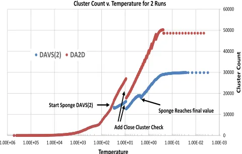
c). Also clusters were removed if they were too small or if their centers were too close. As seen in Fig. 6, this close cluster check was only used at low temperatures i.e. at a distance scale when clusters were resolved. Clusters are considered final when the freezing factor FF given below in (15) is small. Note at convergence <Mx(k)> are either 1 or

zero whereas at any “non-zero” temperature the <Mx(k)>

sum to 1 for each k and are interpreted as probabilities that are resolved at low temperature. All clusterings are finished with a set of annealing iterations where there is no splitting but one just waits that all clusters have “freezing fraction”

FF < 0.002 (most are much smaller than this). The final temperature for this is around T ~ 0.01.

FF(k) = ∑x=1N <Mx(k)> ( 1 - <Mx(k)> ) / N (15)

The scale represented by sponge cutoff c is much smaller than initial temperature T∞ and so we started the clustering with no sponge factor and then introduce it a lower temperature and in fact anneal it to reach its final value at low temperature. In example given later in Fig. 6, the desired sponge cutoff of 2 was reached at T = 2 after being introduced as a cutoff of 45 at T = 30.

In the LC-MS problem, the variance in m/Z is much smaller than that of RT and if used directly would lead to anomalies as formalism designed for circular clusters. So we adjusted above formalism to make the variance in m/Z anneal from a large value at T∞ to the desired value at T = 12. Note that for LC-MS the variances are the “real values” and so temperature has a natural scale with T=1 as natural “tipping point”.

between compute units (processes or threads) when the equations above consist of parallel arithmetic and global reductions that can be implemented by either MPI or iterative MapReduce [17, 32, 33]. This approach works well for initial values of temperature up to around 512 clusters. However as temperatures decrease the <Mx(k)> change

character and each point becomes associated with a few clusters (an average of 8 out of ~25000 in example below). Thus calculating terms like ∑x=1N <Mx(k)> as a sum over all

clusters becomes inefficient and an unnecessary memory use. Rather one uses a data structure that only keeps the <Mx(k)>

for clusters whose centers are near each point. Further one can exploit parallelism over clusters and both calculate and split clusters separately for the above equations in different regions. This leads to a familiar “local geometric” structure with points divided so nearby points are in the same process and local communications are used for point/clusters which are near the boundary between geometric domains. In LC-MS case, this geometric structure was implemented in one dimension with m/Z splits. One finds a difficulty as a given decomposition may not be best for both point and cluster parallelism; this is well known for example in particle in the cell computations in scientific simulations. In our current results we implement the cluster parallelism for the MPI processes but not the thread parallelism. We kept the decomposition with equal number of points in each process; this led to about a factor of two load imbalance in number of clusters. We can improve this but current approach gives satisfactory performance for current LC-MS problems.

In the LC-MS problem, we repeated the steps above 2 or 3 times to get presented results. After first step, we took the peaks assigned to “sponge cluster” (k =0) and identified clusters in it that had been incorrectly split in first step. The new clusters were merged with those from first step by annealing the combined sample starting not at T∞ but rather a low temperature T ~ 0.2. This was done at most twice in results presented here.

III. TECHNICAL EVALUATION OF DAVSALGORITHM

A. Clustering Methods

This evaluation section includes several clustering methods. There are DAVS(c) which are the parallel multi-cluster deterministic annealing introduced in this paper with cutoff c so that all clusters are trimmed with all peaks satisfying ∆2D(x) ≤ c2 where

∆2D(x) = ((m/Z|cluster center – m/Z|x )/ δ(m/Z))2

+ ((RT|cluster center – RT|x )/ δ(RT))2 (16)

Here previous analysis of the measurement of known peaks (landmarks) gave D(m/Z) = 5.98 10-6 _{and D(RT) = 2.35}

where δ(m/Z) = D(m/Z) . (m/Z) and δ(RT) = D(RT) are 3 times standard deviation of measurement determined by study of landmark peaks. We present results for c = 1, 2 and 3 although latter case does not appear in all analyses as we consider c=3 as so large that many “incorrect” peaks are assigned to clusters. This extends Medea, which is the

trimmed deterministic annealing algorithm described in [9] where deterministic annealing is applied separately to each trimmed cluster.

DA2D is the identical parallel multi-cluster deterministic annealing algorithm run without any trimming. It is a modern implementation of the algorithm introduced in [13-15].

Mclust is a model-based clustering algorithm [34] whose use for this problem is described in [9].

Landmarks are a collection of reference peaks (obtained by identifying a subset of peaks using MS/MS peptide sequencing) used to calibrate and evaluate methods.

B. Computer Systems Used

We used two Indiana University Clusters Madrid and Tempest specified below. These are running Windows HPC Server with parallelism from MPI (using MPI.Net [35] on top of Microsoft MPI) and TPL [36] for thread parallelism. All codes were written in C#. The results should be similar on Linux with Java or C++ coding.

Tempest: 32 nodes, each 4 Intel Xeon E7450 CPUs at

2.40GHz with 6 cores, totaling 24 cores per node; 48 GB node memory and 20Gbps Infiniband network connection

Madrid: 8 nodes, each 4 AMD Opteron 8356 at

2.30GHz with 4 cores, totaling 16 cores per node; 16GB node memory and 1Gbps Ethernet network connection

C. DarTB Dataset

Plasma samples from tuberculosis cases and controls were collected at Dar es Salaam, Tanzania, as part of the Gates Grand Challenges in Global Health GC-13 project on pattern-based proteomic characterization of the epidemiology (prevalence and incidence) of diseases of major importance in the developing world. The DarTB dataset consists of 20 TB case and 20 healthy control plasma samples collected at Dar es Salaam, Tanzania. The samples were shipped to The Broad Institute where they are run through a sample processing pipeline starting with immunoaffinity depletion of the top 14 abundant human proteins using an Agilent MARS-14 depletion column. The depleted plasma is passed through a low molecular weight filter and subjected to reduction, alkylation and trypsin digestion. The digested sample is then fractionated into ten fractions using a basic pH reverse phase column. Fractions 5, 6, and 7 are analyzed via LC-MS on a Thermo LTQ-FT using a 98 min gradient. The resulting 120 raw files were analyzed using the algorithms here. The DarTB dataset contained a grand total of 653,741 peaks in 6 charge states. The full analysis of all data is available [37] but here we focus on the largest charge 2 dataset with 241,605 peaks.

D. Structure of Data

Figs. 1 and 2 illustrate the nature of the data to be clustered. As the error in m/Z is proportional to the inverse of this quantity, we define new 2D positions (x, y) rather than (m/Z, RT)

x = ln(m/Z) / D(m/Z)

with D(m/Z) = 5.98 10-6 _{and D(RT) = 2.35 as discussed}

below (16). By using x and y as defined above, we get reduced variables which should give circular clusters with same size in each dimension. Note this change of variables is only used for display purposes. As described we directly use m/Z and RT as coordinates in the clustering and account for position dependent error by calculating the value of δ(m/Z) (and the fixed δ(RT)) dynamically for each cluster center position. The much smaller value of D(m/Z) compared to D(RT), makes the reduced space very much larger in x than y direction. This would distort the clustering algorithm at large temperatures. Thus as described, we anneal the value of D(m/Z) starting at “infinite” temperature with a large value.

E. Parallelism

Fig. 3 illustrates two aspects of parallel performance. Firstly that MPI parallelism outperforms that coming from threads (compare green and blue). Secondly that we get higher performance (compare red and green) when we use

the cluster parallelism described

in section II. Figure 3 only looks at parallelism within a single 16 core node whereas Figs. 4 and 5 extends this to up to 32 nodes where

the network overheads impact performance on the runs with larger parallelism. This is especially true on the Madrid cluster which only has Ethernet network links whereas Tempest has Infiniband. Again we find MPI outperforms threading but as described earlier, we only implemented the cluster parallelism (used in all runs in this figure) with MPI. Several of these runs use a mix of thread and MPI parallelism; threads implement peak parallelism and MPI peak and cluster parallelism. All DAVS(3) runs in Figs. 3 to 5 used the efficient model where each peak x only stores the occupation probability Mx(k) for relevant (i.e.

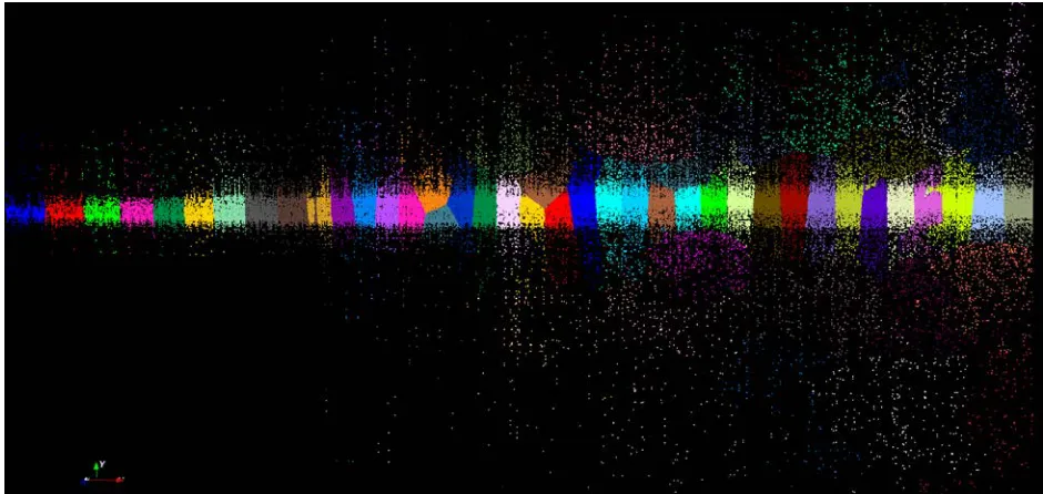
nearby) clusters k. Throughout the run (from 1 to around 25200 clusters in figures), the mean number of clusters Figure 2. A tiny fragment of clustered space for a full DAVS(1) run.

The orange triangles are sponge peaks outside any cluster. The colored hexagons are peaks inside clusters with the white hexagons being determined cluster centers. Each cluster is colored differently. This comes from 241605 peak charge 2 clustering.

Figure 3. Parallelism within a Single Node of Madrid Cluster. A set of runs on 241605 peak data with a single node with 16 cores with either threads or MPI giving parallelism. Parallelism is either number of threads or number of MPI processes.

stored for each peak averaged at most 8 which is < 0.1% of average number of clusters.

Note that parallel clustering has

a) Inefficiencies in that it is not optimally load balanced. We currently decompose problem so there are equal number of peaks in each process. This leads to a factor of 2-4 variation in number of clusters per node. For example the case with 32 MPI processes in Fig. 4 finishes with an average of 789 clusters per node while the minimum number is 511and the maximum 1391. b) Efficiencies as it naturally spreads splitting over the full

region of peaks and this implies that cases with just one MPI process (and any number of threads) need slower annealing to get same number of clusters as runs with more than 4 MPI processes.

The parallel performance is currently limited by the load imbalance effect (a) and MPI communication overheads so that 64 way parallelism is good choice for this 241,605 peak dataset on Madrid and 120 way (30 Tempest nodes with 4 MPI processes in each node) gives best speedup on Tempest. There is also the usual effects that memory bandwidth limits the useful parallelism on each node. We intend tests on

larger datasets where higher levels of parallelism will be optimal. The “production” execution time used in runs reported here vary from 2 to 10 hours (dependent on annealing schedule) on the 8 node Madrid cluster which has rather old (2008) AMD processors. Tempest is a factor 1.8 faster.

IV. DAVS PROTEOMICS EVALAUTION

A. Characteristics of Clustering Solutions

We present in table 1, some summary statistics over the clusterings considered here. We list errors which are just the mean squared scaled differences between peaks and cluster centers averaged over peaks x in cluster.

Error(m/Z) = ((m/Z|cluster center – m/Z|x )/ δ(m/Z))2 (18)

Error(RT) = ((RT|cluster center – RT|x )/ δ(RT))2 (19)

which added together give ∆2D(x) defined in (16). Table 1: Basic Statistics

Method Number

Clusters

Number of Clusters with given occupation count

Count > 30 Scaled Error

1 2 >2 >30 m/Z RT

DAVS(1) 73238 42815 10677 19746 1111 0.036 0.056 DAVS(2) 54055 19449 10824 23781 1257 0.079 0.100 DAVS(3) 41929 13708 7163 21058 1597 0.247 0.290 DA2D 48605 13030 9563 22545 1254 0.100 0.120 Mclust 84219 50689 14293 19237 917 0.021 0.041 One can calculate a much more reliable mean (as used later in comparison with Landmark clusters) by an additional cut like ∆2D(x) ≤ 1.2 to remove outliers.

Figure 4. Speedups for several runs on Madrid from sequential through 128 way parallelism defined as product of number of threads per process and number of MPI processes. We look at different choices for MPI processes which are either inside nodes or on separate nodes. For example 16-way parallelism shows 3 choices with thread count 1:16 processes on one node (the fastest), 2 processes on 8 nodes and 8 processes on 2 nodes.

Figure 5. Speedups for several runs on Tempest from 8-way through 384 way MPI parallelism with one thread per process. We look at different choices for MPI processes which are either inside nodes or on separate nodes.

0 10000 20000 30000 40000 50000 60000

1.00E-03 1.00E-02 1.00E-01 1.00E+00 1.00E+01 1.00E+02 1.00E+03 1.00E+04 1.00E+05 1.00E+06

Cl

us

te

r Co

un

t

Temperature

Cluster Count v. Temperature for 2 Runs

DAVS(2) DA2D

Start Sponge DAVS(2)

Add Close Cluster Check

Sponge Reaches final value

Note both DAVS(c) and DA2D start with one cluster and

then split automatically as temperature is reduced. This is illustrated earlier in Fig. 1 showing a high temperature with 60 clusters. Figure 6 shows how the number of clusters changes with temperature. The following set of figures describe the characteristics of the different solutions. Figures 7 and 8 plots the squared distance distributions scaled by δ(m/Z) for m/Z and δ(RT) for RT in two dimensions i.e. the ordinate is ∆2D(x). These include the expectation of a

Gaussian distribution in ∆2D(x) with standard deviation of 1/3

in both m/Z and RT. It is normalized at ∆2D(x) ~ 0.5 to the

DAVS distributions that are similar in value there.

We note that the four deterministic annealing solutions are quite similar at small values of ∆2D(x) ≤ 1 and in each

case we see a peak above the Gaussian for ∆2D(x) ≤ 0.1. Note

the parallel DAVS(1) precisely enforces the cut ∆2D(x) ≤ 1.

Mclust has sharper distributions but as is made clearer with later data, it misses several clusters and many peaks that are properly associated with a given cluster. Figure 9 shows a histogram of occupation counts for the clustering methods. Mclust tends to lie below the deterministic annealing solutions for the larger clusters as it systemically underestimates the peaks in each cluster as shown in rapid fall off in ∆2D(x) of Figs. 7 and 8.

B. Quality of Determination of Landmark Peaks

Table 2: Charge 2 Landmark Peaks >3 Peaks in Cluster (at least 3 match)

# Peaks Method

To ta l # Clu st er s wi th > 1 p ea ks N um ber S in gl et on Cl ust er s ( 1 p ea k) N um be r L an dm ar k Clu st er s F ou nd Scaled Error # La nd m ar k P ea ks # N on L an dm ar k Pe aks m/Z RT

241605 DAVS(1) 30424 42815 1025 0.039 0.059 24825 6779

241605 DAVS(2) 34606 19449 1033 0.044 0.066 25012 7641

241605 DAVS(3) 28221 13708 1038 0.085 0.112 24939 9825

241605 DA2D 35472 13134 1033 0.044 0.067 24996 7606

241605 Mclust 33530 50948 1007 0.035 0.051 23432 4945

26916 Land mark

1263 228 1034 0.000 0.000 25151 0

Table 3: Charge 2 Landmark Peaks >40 Peaks in Cluster (at least 36 match)

Method Number Landmark Clusters Found Scaled Error ∆2D(x) ≤ 1.2

# Landmark Peaks # Non Landmark Peaks

m/Z RT

DAVS(1) 125 0.021 0.028 6468 831

DAVS(2) 126 0.025 0.032 6563 956

DAVS(3) 129 0.028 0.041 6695 1093

DA2D 126 0.025 0.032 6579 964

Mclust 111 0.021 0.031 5597 584

Landmark 129 0.000 0.000 6675 0

1 10 100 1000 10000 100000

0 20 40 60 80 100 120 140

#Cl us te rs w ith O cc upa tio n Co un t

Occupation Count (Peaks in Cluster)

DAVS(1) DAVS(2) DA2D Mclust Golden

Figure 9. Histograms of number of peaks in clusters for 4 clustering methods and the landmark set. Note lowest bin is clusters with one member peak, i.e. unclustered singletons. For DAVS these are Sponge peaks. 1 10 100 1000 10000 100000

0 0.5 1 1.5 2 2.5 3 3.5 4 4.5 5

Pe ak Co un t i n Bi n

Scaled 2D Distance Squared ∆2D(x)

4 Clustering Methods: Occupation Count > 5 Peaks

Squared Distance Peak to Center DAVS(1) 8664

DAVS(2) 8755

DA2D 8749

Mclust 8194

Landmark 996

Gaussian

Method Name Followed by # Clusters

Figure 8. Histograms of ∆2D(x) for 4 different clusters methods, and the landmark set plus expectation for a Gaussian distribution with standard deviations given as 1/3 in the two directions. The “Landmark” distribution correspond to previously identified peaks used as a control set. Note DAVS(1) and DAVS(2) have sharp cut offs at ∆2D(x) = 1 and 4 respectively. Only clusters with more than 5 peaks are plotted. 1 10 100 1000 10000

0 0.5 1 1.5 2 2.5 3 3.5 4

Pe ak Co un t i n Bi n

Scaled 2D Distance Squared ∆_2D(x) 4 Clustering Methods: Occupation Count > 50 Peaks

Squared Distance Peak to Center DAVS(1) 177 DAVS(2) 224 DA2D 225 Mclust 120 Landmark 58 Gaussian

Method Name Followed by # Clusters

Figure 7. Histograms of ∆2D(x) for 4 different clusters methods, and the landmark set plus expectation for a Gaussian distribution with standard deviations given as δ(m/z)/3 and δ(RT)/3 in two directions. The “Landmark” distribution correspond to previously identified peaks used as a control set. Note DAVS(1) and DAVS(2) have sharp cut offs at

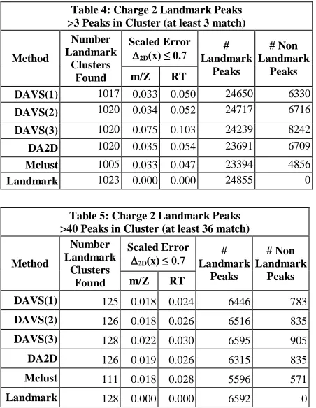
We analyzed the reliability of determining the known Landmark peaks in identical fashion for each clustering method. The results are presented in Tables 2 to 5 which have different selections on cluster size and on later cut in ∆2D(x) used to determine cluster centers. The Landmark

peaks are labeled and we determined for each Landmark cluster, the cluster that best matched it for each of 4 clustering methods. Then we found the center of the cluster, which averaged all peaks whose value of ∆2D(x) was ≤ cut

given in table; this cut improved accuracy (for higher cutoffs c= 2 or 3) as recorded in tables 2 and 3 in the scaled error in each dimension. Reducing value of this cut increases accuracy at cost of reducing number of clusters found as shown in tables 4 and 5 which have cut ∆2D(x) ≤ 0.7. The

tables also record the number of Landmark and Non-Landmark peaks in each cluster after this cut. The Deterministic Annealing methods DAVS and DA2D are quite similar with DAVS(3) recognizing more clusters in case where we restrict clusters to those with at least 40 members. However this comes with slightly larger errors. The systematics suggest that the methods can be ordered DAVS(3), DA2D, DAVS(2), DAVS(1), Mclust in ability to identify Landmark clusters with error decreasing as number of cluster do. Reducing the cut c in DAVS(c) below 1 or similarly adding a low ∆2D(x) cut to a DAVS( c ≥ 1)

clustering gives results that have errors that are similar to Mclust but still find substantially more Landmark clusters than Mclust as seen clearly in tables 4 and especially 5.

It is interesting that the traditional (deterministic annealing) clustering DA2D using a model for cluster shape but no cutoff c, can give excellent results shown in tables 3-5

either by applying a cutoff on ∆2D(x) in cluster center

determination or by restricting the sample to well determined clusters with many peaks such as cut on 40 members in table 3. Note the selection in tables 3 and 5 required that the Landmark cluster had at least 40 peaks, and that after cuts the matching DAVS(c), DA2D or Mclust cluster had at least 36 of the Landmark peaks in it. For Tables 2 and 4, we required at least 3 peaks in Landmark cluster and that the associated clustering solution also had at least 3 Landmark peaks.

V. CONCLUSIONS

We have combined results from robust statistics, model-dependent clustering [38], and parallel computing to produce an accurate automatic approach to analyzing a cohort of multiple biological samples in proteomic biomarker discovery. This required new ideas such as annealing of the model (error requirement) and parallelism over both clusters and peaks. It also combines into a single system known ideas (in the small deterministic annealing community as cited in section II) such as intrinsic cluster probabilities p(k) that had not to our knowledge been integrated before in a large scale parallel “production quality” system. The peaks are found in an unbiased way that requires no initial priming (i.e. no initial guesses at centers). All clusters are essentially located at the overall peak centroid at the start (large temperature) and emerge as temperature lowers from examination of the stability of existing clusters to splitting as shown in Fig. 6. The splitting is determined from the eigenvalues of second order Taylor expansion and not as in some approaches by trial and error with separated centers. The open source software is available [39] although it is now written in C# and we are working on a more broadly useful distribution in R, Java or C++. There are more details of current analysis available at [37].

Large-scale proteomic biomarker discovery efforts using label-free LC-MS experiments are beset with relatively high false-positive rates. The improved performance of DAVS(c) in identifying landmark clusters, we hope, will translate to lowering false-positive rates in biomarker discovery experiments. In addition, the scalable parallel implementation will enable analysis of larger and larger sample cohorts leading to more robust biomarker discovery. As markers discovered using such efforts are validated in the laboratory, there will be more data available to directly evaluate the effectiveness of our new clustering algorithms

Furthermore, combining the recent improvements in high throughput mass spectrometry with these parallel clustering algorithms will empower biomarker discovery with fast turnaround times, and moves us a step closer to the promise of near real-time response to disease outbreaks.

Future work will highlight extension of the analysis to much larger proteomics datasets and extend our work to cloud platforms [32, 33]. Further we will enhance the parallel load balancing that needs to reconcile distributions that optimize peak and cluster decompositions. This has similarities with other better studied parallel algorithms such as those used in particle in the cell simulations. We believe that large scale data analytics such as that presented here

Table 4: Charge 2 Landmark Peaks >3 Peaks in Cluster (at least 3 match)

Method

Number Landmark

Clusters Found

Scaled Error ∆2D(x) ≤ 0.7

# Landmark

Peaks

# Non Landmark

Peaks

m/Z RT

DAVS(1) 1017 0.033 0.050 24650 6330

DAVS(2) 1020 0.034 0.052 24717 6716

DAVS(3) 1020 0.075 0.103 24239 8242

DA2D 1020 0.035 0.054 23691 6709

Mclust 1005 0.033 0.047 23394 4856

Landmark 1023 0.000 0.000 24855 0

Table 5: Charge 2 Landmark Peaks >40 Peaks in Cluster (at least 36 match)

Method

Number Landmark

Clusters Found

Scaled Error ∆2D(x) ≤ 0.7

# Landmark

Peaks

# Non Landmark

Peaks

m/Z RT

DAVS(1) 125 0.018 0.024 6446 783

DAVS(2) 126 0.018 0.026 6516 835

DAVS(3) 128 0.022 0.030 6595 905

DA2D 126 0.019 0.026 6315 835

Mclust 111 0.018 0.028 5596 571

present novel challenges for the parallel computing community and we will package kernel versions of software to be used in benchmark analyses.

ACKNOWLEDGMENTS

GCF is partially supported by Microsoft and by NSF via FutureGrid Grant No. 0910812. SP thanks MoS&PI, DBT and DST, Government of India, for financial support.

REFERENCES

[1] M. S. Boguski and M. W. McIntosh, "Biomedical informatics for proteomics," Nature, vol. 422, pp. 233-237, 2003.

[2] J. D. Jaffe, D. R. Mani, K. C. Leptos, G. M. Church, M. A. Gillette, and S. A. Carr, "PEPPeR, a platform for experimental proteomic pattern recognition," Molecular & Cellular Proteomics, vol. 5, pp. 1927-1941, 2006.

[3] R. Malik, K. Dulla, E. A. Nigg, and R. Körner, "From proteome lists to biological impact–tools and strategies for the analysis of large MS data sets," Proteomics, vol. 10, pp. 1270-1283, 2010.

[4] Y. Mohammed, E. Mostovenko, A. A. Henneman, R. J. Marissen, A. M. Deelder, and M. Palmblad, "Cloud Parallel Processing of Tandem Mass Spectrometry Based Proteomics Data," Journal of Proteome Research, vol. 11, pp. 5101-5108, 2012.

[5] J. C. de Groot, M. W. Fiers, R. C. van Ham, and A. H. America, "Post alignment clustering procedure for comparative quantitative proteomics LC‐MS Data," Proteomics, vol. 8, pp. 32-36, 2008. [6] B. L. LaMarche, K. L. Crowell, N. Jaitly, V. A. Petyuk, A. R. Shah, A.

D. Polpitiya, et al., "MultiAlign: a multiple LC-MS analysis tool for targeted omics analysis," BMC bioinformatics, vol. 14, p. 49, 2013. [7] F. Saeed, T. Pisitkun, M. A. Knepper, and J. D. Hoffert, "An efficient

algorithm for clustering of large-scale mass spectrometry data," in Bioinformatics and Biomedicine (BIBM), 2012 IEEE International Conference on, 2012, pp. 1-4.

[8] X. Kang, Y. Xu, X. Wu, Y. Liang, C. Wang, J. Guo, et al., "Proteomic fingerprints for potential application to early diagnosis of severe acute respiratory syndrome," Clinical chemistry, vol. 51, pp. 56-64, 2005. [9] Rudolf Fruhwirth, D. R. Mani, and Saumyadipta Pyne, "Clustering

with position-specific constraints on variance: Applying redescending M-estimators to label-free LC-MS data analysis," BMC Bioinformatics, vol. 12, p. 358, 2011.

[10] Rudolf Fruhwirth and Wolfgang Waltenberger, "Redescending M-estimators and Deterministic Annealing, with Applications to Robust Regression and Tail Index Estimation," AUSTRIAN JOURNAL OF STATISTICS, vol. 3 & 4, pp. 301–317, 2008.

[11] P. J. Huber, Robust statistical procedures vol. 68: SIAM, 1996. [12] S. Z. Li, "Robustizing robust M-estimation using deterministic

annealing," Pattern Recognition, vol. 29, pp. 159-166, 1996.

[13] Ken Rose, Eitan Gurewitz, and Geoffrey Fox, "A deterministic annealing approach to clustering," Pattern Recogn. Lett., vol. 11, pp. 589--594, 1990.

[14] Kenneth Rose, Eitan Gurewitz, and Geoffrey C Fox, "Statistical mechanics and phase transitions in clustering," Phys. Rev. Lett., vol. 65, pp. 945--948, Aug 1990.

[15] Ken Rose, "Deterministic Annealing for Clustering, Compression, Classification, Regression, and Related Optimization Problems," Proceedings of the IEEE, vol. 86, pp. 2210--2239, 1998.

[16] Geoffrey C. Fox, "Large scale data analytics on clouds," presented at the Proceedings of the fourth international workshop on Cloud data management, Maui, Hawaii, USA, 2012.

[17] Yang Ruan, Saliya Ekanayake, Mina Rho, Haixu Tang, Seung-Hee Bae, Judy Qiu, et al., "DACIDR: Deterministic Annealed Clustering with Interpolative Dimension Reduction using Large Collection of 16S rRNA Sequences," presented at the ACM Conference on Bioinformatics, Computational Biology and Biomedicine (ACM BCB), Orlando, Florida, 2012.

[18] Geoffrey C. Fox, "Deterministic annealing and robust scalable data mining for the data deluge," presented at the Proceedings of the 2nd

international workshop on Petascale data analytics: challenges and opportunities, Seattle, Washington, USA, 2011.

[19] Geoffrey Fox, Seung-Hee Bae, Jaliya Ekanayake, Xiaohong Qiu, and H. Yuan, Parallel Data Mining from Multicore to Cloudy Grids: IOS Press, Amsterdam, 2009.

[20] Geoffrey Fox, "Robust Scalable Visualized Clustering in Vector and non Vector Semimetric Spaces," Parallel Processing Letters, vol. To be published, May 17 2013.

[21] T. Hofmann and J. M. Buhmann, "Pairwise Data Clustering by Deterministic Annealing," IEEE Transactions on Pattern Analysis and Machine Intelligence, vol. 19, pp. 1-14, 1997.

[22] R. Frühwirth, W. Waltenberger, K. Prokofiev, T. Speer, P. Vanlaer, E. Chabanat, et al., "New vertex reconstruction algorithms for CMS," arXiv preprint physics/0306012, 2003.

[23] A. Rangarajan, "Self-annealing and self-annihilation: unifying deterministic annealing and relaxation labeling," Pattern Recognition, vol. 33, pp. 635-649, 2000.

[24] A. T. Nguyen, "Identification of Air Traffic Flow Segments via Incremental Deterministic Annealing Clustering," Ph.D., Electrical Engineering, University of Maryland, 2012.

[25] G. YANG and S. SHI, "Parallel clustering algorithm by deterministic annealing [J]," Journal of Tsinghua University (Science and Technology), vol. 4, p. 011, 2003.

[26] E. Kim, W. Wang, H. Li, and X. Huang, "A parallel annealing method for automatic color cervigram image segmentation," in Medical Image Computing and Computer Assisted Intervention, MICCAI-GRID 2009 HPC Workshop, 2009.

[27] X.-L. Yang, Q. Song, and Y.-L. Wu, "A robust deterministic annealing algorithm for data clustering," Data & Knowledge Engineering, vol. 62, pp. 84-100, 7// 2007.

[28] L. Angelini, G. Nardulli, L. Nitti, M. Pellicoro, D. Perrino, and S. Stramaglia, "Deterministic annealing as a jet clustering algorithm in hadronic collisions," Physics Letters B, vol. 601, pp. 56-63, 2004. [29] X. Yang, A. Cao, and Q. Song, "A new cluster validity for data

clustering," Neural processing letters, vol. 23, pp. 325-344, 2006. [30] F. Rossi and N. Villa-Vialaneix, "Optimizing an organized modularity

measure for topographic graph clustering: a deterministic annealing approach," Neurocomputing, vol. 73, pp. 1142-1163, 2010.

[31] S. Zhong and J. Ghosh, "A comparative study of generative models for document clustering," in Proceedings of the workshop on Clustering High Dimensional Data and Its Applications in SIAM Data Mining Conference, 2003.

[32] J.Ekanayake, H.Li, B.Zhang, T.Gunarathne, S.Bae, J.Qiu, et al., "Twister: A Runtime for iterative MapReduce," presented at the Proceedings of the First International Workshop on MapReduce and its Applications of ACM HPDC 2010 conference June 20-25, 2010, Chicago, Illinois, 2010.

[33] Thilina Gunarathne, Bingjing Zhang, Tak-Lon Wu, and Judy Qiu, "Scalable Parallel Computing on Clouds Using Twister4Azure Iterative MapReduce " Future Generation Computer Systems vol. 29, pp. 1035-1048, 2013.

[34] Chris Fraley and Adrian E. Raftery, "Enhanced Model-Based Clustering, Density Estimation, and Discriminant Analysis Software: MCLUST," Journal of Classification, vol. 20, pp. 263-286, 2003. [35] Open Systems Lab Indiana University Bloomington. (2008). MPI.NET

Message Passing for C#. Available: http://osl.iu.edu/research/mpi.net/

[36] Judy Qiu and Seung-Hee Bae, "Performance of Windows Multicore Systems on Threading and MPI " Concurrency and Computation: Practice and Experience, vol. Special Issue for FGMMS Frontiers of GPU, Multi- and Many-Core Systems 2010, 2011.

[37] Geoffrey Fox , D. R. Mani, and Saumyadipta Pyne. (2013, June 22). Detailed Results of Evaluation of DAVS(c) Deterministic Annealing Clustering and its Application to LC-MS Data Analysis Available: http://grids.ucs.indiana.edu/ptliupages/publications/DAVS2.pdf [38] G. Fung. (2001). A comprehensive overview of basic clustering

algorithms. Available: http://www.cs.wisc.edu/~gfung/clustering.ps.gz