On Graphs with Same Distance Distribution

(1)

http://www.scirp.org/journal/am ISSN Online: 2152-7393

ISSN Print: 2152-7385

On Graphs with Same Distance Distribution

Xiuliang Qiu

1*

_{, Xiaofeng Guo}

2,3

1_{Chengyi University College, Jimei University, Xiamen, China} 2_{School of Mathematical Sciences, Xiamen University, Xiamen, China}

3_{College of Mathematics and System Sciences, Xinjiang University, Urumchi, China}

Abstract

In the present paper we investigate the relationship between Wiener number

W, hyper-Wiener number R, Wiener vectors WV , hyper-Wiener vectors HWV, Wiener polynomial H , hyper-Wiener polynomial HH and dis-

tance distribution DD of a (molecular) graph. It is shown that for

connected graphs G and *

G , the following five statements are equivalent:

1)

( )

*

DD G =DD G , 2) WV G

( )

=WV G

( )

* , 3) HWV G

( )

=HWV G

( )

* , 4)

( )

*

H G =H G , 5)

( )

*

HH G =HH G ; and if G and G* have same dis-

tance distribution DD then they have same W and R but the contrary is

not true. Therefore, we further investigate the graphs with same distance distribution. Some construction methods for finding graphs with same distance distribution are given.

Keywords

Distance Distribution, Distance Matrix, Wiener Vector, Hyper-Wiener Vector

1. Introduction

The Wiener index is one of the oldest topological indices of molecular structures. It was put forward by the physico-chemist Harold Wiener [1] in 1947. The Wiener index of a connected graph G is defined as the sum of distances

between all pairs of vertices in G:

( )

{ } ( ),

( )

, .

G u v V G

W W G d u v

⊆

= =

∑

where V G

( )

is the vertex set of G, and d_G

( )

u v, is the distance between

vertices u and v in G.

As an extension of the Wiener index of a tree, Randić [2] introduced Wiener matrix W and hyper-Wiener index R of a tree. For any two vertices i j, in

How to cite this paper: Qiu, X.L. and Guo, X.F. (2017) On Graphs with Same Distance Distribution. Applied Mathematics, 8, 799- 807.

https://doi.org/10.4236/am.2017.86062

Received: April 18, 2017 Accepted: June 16, 2017 Published: June 19, 2017

http://creativecommons.org/licenses/by/4.0/

(2)

T, let

π

( )

i j, denote the unique path in T with end vertices i j, and the

length dij, let T1,π( )i j, and T2,π( )i j, denote the components of T−E

(

π

( )

i j,

)

containing i and j, respectively, and let n_1,_π_{( )}_{i j}_, and n_2,_π_{( )}_{i j}_, denote the

numbers of the vertices in T1,π( )i j, and T2,π( )i j, , respectively. Then the Wiener

matrix W and the hyper-Wiener number R of T can be given by W =

( )

wij ,

( ) ( )

1, , 2, ,

ij i j i j

w =n_π ⋅n _π , and R=

∑

i j< wij.

In Refs. [3] [4], Randic and Guo and colleagues further introduced the higher Wiener numbers and some other Wiener matrix invariants of a tree T. The

higher Wiener numbers can be represented by a Wiener number sequence

1_{W W W}_,2 _,3 _,_, where

, , i j k

ij d k i j

W=

∑

_{= <} w . It is not difficult to see 1W =W, and

1,2, k k

R=

∑

₌ _W.

After the hyper-Wiener index of a tree was introduced, many publications [5]-[11] have appeared on calculation and generalization of the hyper-Wiener index. Klein et al. [5] generalized the hyper-Wiener index so as to be applicable to any connected structure. Their formula for the hyper-Wiener index R of a

graph G is

( )

{ } ( )

(

( )

)

2 ,

1

, , .

2 u v V G G G

R R G d u v d u v

⊆

= =

∑

+

The relation between Hyper-Wiener and Wiener index was given by Gutman [11].

The Hosoya polynomial H G

( )

of a connected graph G was introduced by

Hosoya [12] in 1988, which he named as the Wiener polynomial of a graph:

(

)

(

)

0

, , k,

k

H H G x d G k x

≥

= =

∑

where d G k

(

,

)

is the number of pairs of vertices in the graph G that are

distance k apart.

In Ref. [13], Cash introduced a new hyper-Hosoya polynomial

(

)

(

) ( )

0

1

, , .

2

k

HH HH G x d G k x

≥

+

= =

∑

The relationship between the Hosoya polynomial and the Hyper-Hosoya polynomial was discussed [13].

The sequence

(

d G

( ) (

,1 ,d G, 2 ,

)



)

is also known (since 1981) as the dis-

tance distribution of a graph G [14], denoted by DD G

( )

. It is easy to see that

(

)

0 ,

k

W =

∑

_≥ k d G k⋅ .

Later the definition of higher Wiener numbers is extended to be applicable to any connected structure by Guo et al. [15]. For a connected graph G with n

vertices, denoted by 1, 2,,n, let wij k, =max

{

dij− +k 1, 0

}

where dij is the distance between vertices i and j. Then k _,

ij k i j

W =

∑

_< w , k=1, 2,, are

called the higher Wiener numbers of G. The vector

(

1W W,2 ,

)

is called the

hyper-Wiener vector of G, denoted by HWV G

( )

. The concept of the Wiener

vector of a graph is also introduced in ref. [15]. For a connected graph G with n vertices, denoted by 1, 2,,n, let Wk =

∑

i j d ij<_, _{( )}=kdij, k=1, 2,. The vector

(

W W1, 2,

)

is called the Wiener vector of G, denoted by WV G

( )

.

Moreover, a matrix sequence

(

( )1 ( )2 ( )3

)

, , ,

(3)

sequence, and their sum 1,2, ( ) ( )

k H

k= =

∑

_W W , called the hyper-Wiener matrix,

are introduced, where ( )1

D

=

W is the distance matrix. A Wiener polynomial

sequence and a weighted hyper Wiener polynomial of a graph are also introduced.

In this paper, based on the results in ref. [15], we study the relation between Wiener number W , hyper-Wiener number R, Wiener vector WV, hyper-

Wiener vector HWV, Hosoya polynomial H, hyper-Hosoya polynomial HH

and distance distribution DD of a graph. It is shown that for connected graphs G and *

G , the the contrary is not true. This means that the distance dis-

tribution of a graph is an important topological index of molecular graphs. Therefore, we further investigate the graphs with same distance distribution. It is shown that the graphs with same vertex number, edge number, and diameter 2 have same distance distribution. Some construction methods for finding graphs with same distance distribution are given.

2. The Relation between

W R WV HWV H HH DD

, ,

,

Let diam G

( )

denote the diameter of a graph G.

Theorem 2.1. Let G and G* be connected graphs. Then the following five

statements are equivalent:

1) G and G* have same distance distribution DD;

2) G and G* have same Wiener vector WV ;

3) G and G* have same hyper-Wiener vector HWV;

4) G and G* have same Wiener polynomial H;

5) G and G* have same hyper-Wiener polynomial HH.

Proof. We shall show the equivalent statements by (1)⇒₍₂₎⇒₍₃₎⇒₍₄₎⇒₍₅₎⇒_(1).

(1)⇒_{(2). By the definitions of} DD and WV ,

( )

(

( ) (

,1 , , 2 ,

)

,

(

,

( )

)

DD G = d G d G  d G diam G , and

( )

(

1, 2, , diam G( )

)

(

1

( )

,1 , 2

(

, 2 ,

)

,

( )

(

,

( )

)

WV G = W W W = d G d G  diam G d G diam G .

Clearly, if

( )

*

DD G =DD G , then WV G

( )

=WV G

( )

* .

(2)⇒_{(3). If}

( )

*

WV G =WV G , then *

* *

,ij ,ij

k i j d k ij k i j d k ij

W =

∑

_< ₌d =W =

∑

_< ₌d

for k=1, 2,,diam G

( )

. So

{

}

{

*

}

* *

, max 1, 0 max 1, 0 ,

k k

ij k ij ij ij k

i j i j i j i j

W=

∑

_<w =

∑

_< d − +k =

∑

_< d − +k =

∑

_<w = W

for k=1, 2,,diam G

( )

. Hence

( )

*

HWV G =HWV G .

(3)⇒_{(4). Suppose}

( )

*

HWV G =HWV G . Then k k *

W = W for k=1, 2,,

and

( )

*

diam G =diam G .

If

( )

*

k=diam G =diam G , then

{

}

(

( )

)

{

}

(

( )

)

* * * *

max 1, 0 ,

k ij i j k ij i j

W d k d G diam G

< < = − + = = = − + =

∑

.

Assume, for 1< ≤ ≤l k diam G

( )

, d G k

(

,

)

=d G k

(

*,

)

. Let k= −l 1. Then

{

}

(

)

{

}

(

)

(

)(

)

1

, 1

max 2, 0 , 1 max 2, 0

, 1 , 2

ij

ij l

ij ij

i j i j d l

i j d k l

W d l d G l d l

d G l d G k k l

−

< < > −

′ < = > −

= − + = − + − +

′ ′

= − + − +

∑

(4)

{

} (

)

{

}

(

)

(

)

(

)

*

1 * * * *

, 1

* * 1

, 1

max 2, 0 , 1 max 2, 0

, 1 , 2

ij

ij l

ij ij

i j i j d l

l i j d k l

W d l d G l d l

d G l d G k k l W

−

< < > −

− ′

< = > −

= − + = − + − +

′ ′

= − + − + =

∑

.

By induction hypothesis,

(

)(

)

*

(

)

(

)

*

, ij 1 , 2 ,ij 1 , 2

i j d< = > −k l′ d G k′ k′− +l = i j d< = > −k l′ d G k′ k′− +l

∑

. So we have

(

)

(

*

)

, 1 , 1

d G l− =d G l− .

Now it follows that

(

)

(

*

)

, ,

d G k =d G k for k=1, 2,, and so

(

)

(

)

(

*

)

(

*

)

0 0

, , k , k ,

k k

H G x =

∑

_≥d G k x =

∑

_≥d G k x =H G x .

(4)⇒(5). By the definitions of Hosoya polynomial H and hyper-Hosoya

polynomial HH, it is easy to see that, if H G x

(

,

)

=H G x

(

*,

)

, then

(

)

(

*

)

, ,

HH G x =HH G x .

(5)⇒_{(1). If}

(

)

(

*

)

, ,

HH G x =HH G x , then

(

)

(

*

)

, ,

d G k =d G k for

1, 2,

k= . Therefore DD G

( )

=DD G

( )

* . □

Theorem 2.2. Let G and G* be two graphs with same distance dis-

tribution. Then G and G* have same W and R.

Proof: By the definitions of DD, W and R,

( )

(

( ) (

,1 , , 2 ,

)

,

(

,

( )

)

DD G = d G d G  d G diam G ,W G

( )

=

∑

_{{ } ( )}u v_, ⊆V GdG

( )

u v, ,

and

( )

_{{ } ( )}

(

2

( )

)

,

1

, ,

2 u v V G G G

R G =

∑

_⊆ d u v +d u v .

Clearly, if

( )

*

DD G =DD G , then W G

( )

=W G

( )

* and R G

( )

=R G

( )

* . 

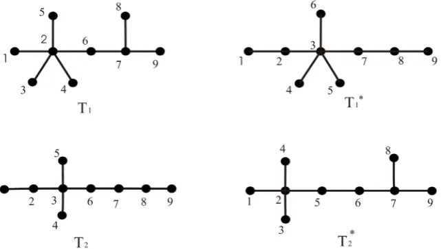
However, the contrary of the theorem doesn’t hold. For instance, the trees T1

and * 1

T (resp. T₂ and T2*) in Figure 1 have same W and R, but they have

different distance distributions.

3. Graphs with Same Distance Distribution

[image:4.595.214.535.495.676.2]

From the above theorems, one can see that, if two graphs G and G* have

Figure 1.

( )

*

1 1 86

W T =W T = ,

( )

*

1 1 166

R T =R T = , DD T

( ) (

₁ = 8,14,6,8

)

,

( )

*

(

)

1 8,13,9,5,1

DD T = .

( )

*

2 2 98

W T =W T = ,

( )

*

2 2 217

R T =R T = ,

( ) (

2 8,10,8,5, 4,1

)

(5)

same distance distribution DD, then they have same W WW WV HWV H, , , , and HH. So it is significant to study the graphs with same distance distribution.

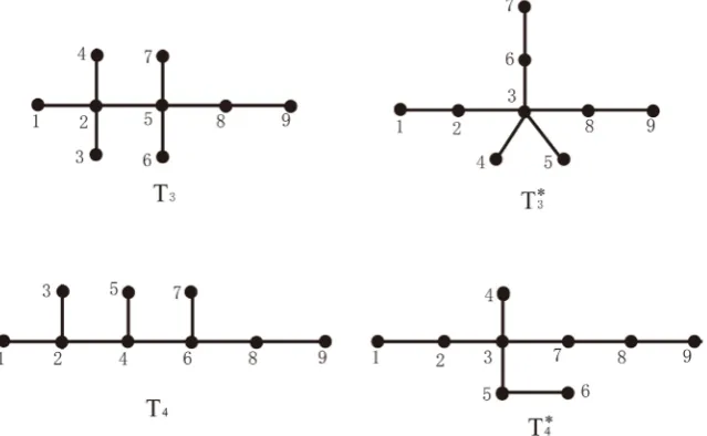
1) The minimum non-isomorphic acyclic graphs with same DD

By direct calculation, we know the minimum non-isomorphic acyclic graphs with same distance distribution are the following two pairs of trees in Figure 2 which have 9 vertices.

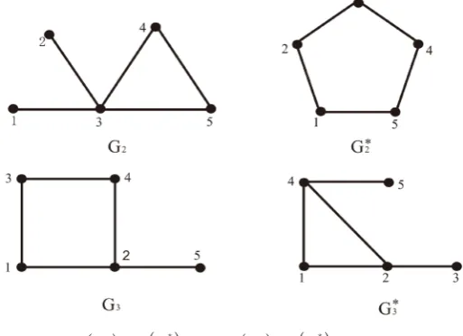
2) The minimum non-isomorphic cyclic graphs with same DD

The minimum non-isomorphic cyclic graphs with same distance distribution are the following graphs with 4 vertices (see Figure 3).

Note that, for the above graphs with same distance distribution, their Wiener matrix sequences and hyper-Wiener matrices are different.

The following theorem gives a class of graphs with same distance distribution. Let n m, be the set of all the graphs with n vertices and m edges.

Theorem 3.1. Let * ,

, n m

G G ∈ , and diam G

( )

=diam G

( )

* =2. Then

( )

*

DD G =DD G .

Proof. Since * ,

, n m

G G ∈ and diam G

( )

=diam G

( )

* =2, we have

Figure 2.

( )

*

3 3 82

W T =W T = ,

( )

*

3 3 149

R T =R T = ,

( )

*

(

)

3 3 8,13,12,3

DD T =DD T = .

( )

* 4 4 92

W T =W T = ,

( )

*

4 4 188

R T =R T = ,

( )

*

(

)

4 4 8,10,10,6, 2

[image:5.595.214.534.334.531.2]

DD T =DD T = .

Figure 3.

( )

*

1 1 8

W G =W G = ,

( )

*

1 1 10

R G =R G = ,

( )

*

( )

1 1 4, 2

(6)

( )

*

,1 ,1

d G =d G =m,

(

)

(

*

)

, 2 , 2

2 n

d G =d G = _{ }−m

  ,

(

)

(

)

*

, , 0

d G k =d G k =

for k≥3, and so DD G

( )

=DD G

( )

* .

Corollary 3.2. If 1

2 2

n n

m n

 _{> >} _{− +}

   

    , then all graphs in n m, have same

distance distribution.

Proof. For ∀ ∈G n m, with 1

2 2

n n

m n

 _{> >} _{− +}

   

    , clearly diam G

( )

≥2. We assert that diam G

( )

=2.

Otherwise, there exist two vertices u v V G, ∈

( )

such that d u v

( )

, ≥3. Let P be a shortest

( )

u v, -path. Then any vertex not on P is not adjacent to at

least one of u and v, and the number of pairs of non-adjacent vertices on P

is equal to

(

V P

( )

−2

)

+

(

V P

( )

−3

)

++ =1

(

V P

( )

−2

)

(

V P

( )

−1 2

)

. So

( )

(

)

(

( )

)

(

( )

)

( )

(

)

(

( )

)

2 1 2

2

2 3 4 2 1

2 2

n

m n V P V P V P

n n

n V P V P n

  ≤_{ }− − − − −     _ _   =_{ }− −_ − − − _ ≤_{ }− +    

, contradicting that

1 2 n m> _{ }− +n

  .

Hence, by Theorem 3.1, if 1 2 n m> _{ }− +n

  , all graphs in n m, have same

distance distribution. □

Let G

V

H denote the graph obtained from vertex-disjoint graphs G and H by connecting every vertex of G to every vertex of H.

Corollary 3.3. Let 1 1 1 1 1, 2 n m,

G G ∈ and G G12, 22∈n m₂, ₂. Then

1 2

1 1

G

V

G and

1 2

2 2

G

V

G have same distance distribution.

Proof. Obviously,

(

1 2

)

(

1 2

)

1 1 2 2 1 2

V G

V

G =V G

V

G =n +n ,

(

1 2

)

(

1 2

)

1 1 2 2 2

diam G

V

G =diam G

V

G = , and

(

1 2

)

(

1 2

)

1 1 2 2 1 2 1 2

E G

V

G = E G

V

G =m +m + ⋅n n . By Theorem 3.1,

(

1 2

)

(

1 2

)

1 1 2 2

DD G

V

G =DD G

V

G .

For graphs with diameter greater than or equal to 2, we will give some construction methods for finding graphs with same distance distribution.

Let G be a connected graph with vertices set

{

v v1, 2,,vn

}

, and let

( )

G =

( )

dij

D be the distant matrix of the graph G. Let G

( )

k i

d v denote the

number of the vertices at distance k from a vertex vi in G, and let

( )

(

1

( )

, 2

( )

, , ( )

( )

)

G G G

G i i i diam G i

DD v = d v d v  d v ) be the distance distribution of v_i

in G.

Theorem 3.4. Let G1 and G2 (resp. G1′ and G2′ ) be the connected

graphs with n1 (resp. n2) vertices and with same distance distribution. For

( )

1 1

v ∈V G , v₂∈V G

( )

₂ , v₁′∈V G

( )

₁′ , and v₂′∈V G

( )

₂′ , let G (resp. G*) be

the graph obtained from G1 and G1′ (resp. G2 and G2′) by identifying v1

and v1′ (resp. v2 and v2′). If DDG1

( )

v1 =DDG2

( )

v2 and

( )

1 1 2 2

G G

DD ′ v′ =DD ′ v′ , then G and G* have same distance distribution.

Proof. It is enough to prove

(

)

(

*

)

, ,

(7)

Clearly,

(

)

(

)

(

)

1

( )

1

( )

1 1 1 , , 1 1

, , , _{i j k i j k} _iG G_j

d G k =d G k +d G k′ +

∑

_{≤ ≤ + =}d v d ′ v′ . Similarly,

(

*

)

(

)

(

)

2

( )

2

( )

2 2 1 , , 2 2

, , , G G

i j

i j k i j k

d G k =d G k +d G k′ +

∑

_{≤ ≤ + =}d v d ′ v′ . Because

( )

1

( )

2

DD G =DD G , DD G

( )

1′ =DD G

( )

2′ , DDG₁

( )

v1 =DDG₂

( )

v2 ,

( )

1 1 2 2

G G

DD ′ v′ =DD ′ v′ , we have d G k

(

,

)

=d G k

(

*,

)

for k=1, 2,. Hence

( )

*

DD G =DD G . □

Theorem 3.5. Let Gi∈n m, , i=1, 2, and let Si ⊂V G

( )

i such that any two vertices in Si have distance less than or equal to 2 in Gi, and S1 = S2 . Let

{ }

i i

G S denote the graph obtained from G_i by contracting vertices in Si to a vertex

s

i. Let

*

i

G be the graph obtained from Gi by adding a new vertex xi and connecting xi to every vertex in Si. If DD G

( )

1 =DD G

( )

2 and

{ }

( )

{ }

( )

1 1 1 2 2 2

G S G S

DD s =DD s , then DD G

( )

1* =DD G

( )

2* .

Proof. Clearly, by the conditions of the theorem,

( )

(

{ }

_{( )}

{ }

_{( )}

)

*

1 2

,1 i i ,1 i i ,

i

G S G S

i i _G i i i i i

DD G =DD G +DD x =DD G + S +d x +d x  ,

1, 2

i= . So, if DD G

( )

1 =DD G

( )

2 and DD G

( )

1′ =DD G

( )

2′ and { }

( )

{ }

( )

1 1 1 2 2 2

G S G S

DD s =DD s , then * * 1 2

G G

DD =DD . □

From Theorem 3.4, we have the following corollary:

Corollary 3.6. Let G G1, 2∈n m, and DD G

( )

1 =DD G

( )

2 . Let H be a con-

nected graph vertex-disjoint with G1 and G2. For v1∈V G

( )

1 , v2∈V G

( )

2 ,

and u∈V H

( )

, let G (resp. G*) be the graph obtained from G₁ (resp. G2)

and H by identifying v₁ and u (resp. v₂ and u). If

( )

1 1 2 2

G G

DD v =DD v , then G and G* have same distance distribution.

From Theorem 3.5, one can obtain graphs with same distance distribution in

, n m

 from graphs in n−1,m s− with same distance distribution by adding a new vertex and some edges.

Figure 4 shows two pairs of graphs with 5 vertices and 5 edges and with same

DD, one of which has diameter 2 and the other has diameter 3.

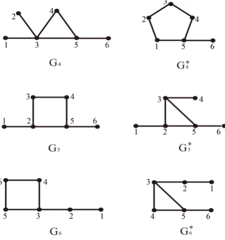
[image:7.595.245.502.503.689.2]

Figure 5 shows three pairs of graphs with 6 vertices and 6 edges and with

Figure 4.

( )

*

2 2 15

W G =W G = ,

( )

*

2 2 20

R G =R G = ,

( )

*

( )

2 2 5,5

DD G =DD G = .

( )

*

3 3 16

W G =W G = ,

( )

* 3 3 23

R G =R G = ,

( )

*

(

)

3 3 5, 4,1

(8)

[image:8.595.257.486.73.318.2]

Figure 5.

( )

* 4 4 26

W G =W G = ,

( )

*

4 4 39

R G =R G = ,

( )

*

(

)

4 4 6,7, 2

DD G =DD G = .

( )

*

5 5 27

W G =W G = ,

( )

* 5 5 42

R G =R G = ,

( )

*

(

)

5 5 6,6,3

DD G =DD G = .

( )

* 6 6 29

W G =W G = ,

( )

*

6 6 49

R G =R G = ,

( )

*

(

)

6 6 6,5,3,1

DD G =DD G = .

same DD, two of which have diameter 3 and the other has diameter 4.

It is easy to see that the graphs in Figure 5 can be obtained from graphs in Figure 3, Figure 4 by the construction methods given in Theorems 3.4, 3.5.

However, the construction methods are not complete. There might be some graphs with same DD which could not be obtained by the above construction

methods.

Open Problem. Is there a construction method for finding all graphs with same distance distribution?

Acknowledgements

This work is jointly supported by the Natural Science Foundation of China (11101187, 61573005, 11361010), the Scientific Research Fund of Fujian Provin-cial Education Department of China (JAT160691).

References

[1] Wiener, H. (1947) Structural Determination of Paraffin Boiling Points. Journal of the American Chemical Society, 69, 17-20.https://doi.org/10.1021/ja01193a005 [2] Randić, M. (1993) Novel Molecular Descriptor for Structure-Property Studies.

Chemical Physics Letters, 211, 478-483. https://doi.org/10.1016/0009-2614(93)87094-J

(9)

Source of Novel Graph Invariants. Journal of Chemical Information and Computer Sciences, 33, 709-716.https://doi.org/10.1021/ci00015a008

[4] Randić, M., Guo, X.F., Oxley, T., Krishnapriyan, h. and Naylor, L. (1994) Wiener Matrix Invariants. Journal of Chemical Information and Computer Sciences, 34, 361-367.https://doi.org/10.1021/ci00018a022

[5] Klein, D.J. and Gutman, I. (1995) On the Definition of the Hyper-Wiener Index for Cycle-Containing Structures. Journal of Chemical Information and Computer Sciences, 35, 50-52.https://doi.org/10.1021/ci00023a007

[6] Lukovits, I. and Linert, W. (1995) A Novel Definition of the Hyper-Wiener Index for Cycles. Journal of Chemical Information and Computer Sciences, 34, 899-902. https://doi.org/10.1021/ci00020a025

[7] Klein, D.J. and Randić, M. (1993) Resistance Distance. Journal of Mathematical Chemistry, 12, 81-95.https://doi.org/10.1007/BF01164627

[8] Li, X.H. (2003) The Extended Hyper-Wiener Index. Canadian Journal of Chemistry, 81, 992-996.https://doi.org/10.1139/v03-106

[9] Klavzar, S., Gutman, I. and Mohar, B. (1995) Labeling of Benzenoid Systems which Reflects the Vertex-Distance Relations. Journal of Chemical Information and Computer Sciences, 35, 590-593.https://doi.org/10.1021/ci00025a030

[10] Cash, G.G., Klavzar, S. and Petkovsek, M. (2002) Three Methods for Calculation of the Hyper-Wiener Index of Molecular Graphs. Journal of Chemical Information and Computer Sciences, 42, 571-576.https://doi.org/10.1021/ci0100999

[11] Gutman, I. (2002) Relation between Hyper-Wiener and Wiener Index. Chemical Physics Letters, 364, 352-356.https://doi.org/10.1016/S0009-2614(02)01343-X [12] Hosoya, H. (1998) On Some Counting Polynominals in Chemistry. Discrete

Ap-plied Mathematics, 19, 239-257.

[13] Cash, G.G. (2002) Relationship between the Hosoya Polynominal and the Hy-per-Wiener Index. Applied Mathematics Letters, 15, 893-895.

[14] Buckley, F. and Superville, L. (1981) Distance Distributions and Mean Distance Problem. Proceedings of Third Caribbean Conference on Combinatorics and Computing, University of the West Indies, Barbados, January 1981, 67-76.

[15] Guo, X.F., klein, D.J., Yan, W.G. and Yeh, Y.-N. (2006) Hyper-Wiener Vector, Wiener Matrix Sequence, and Wiener Polynominal Sequence of a Graph. Interna-tional Journal of Quantum Chemistry, 106, 1756-1761.

(10)

Submit or recommend next manuscript to SCIRP and we will provide best service for you:

Accepting pre-submission inquiries through Email, Facebook, LinkedIn, Twitter, etc. A wide selection of journals (inclusive of 9 subjects, more than 200 journals)

Providing 24-hour high-quality service User-friendly online submission system Fair and swift peer-review system

Efficient typesetting and proofreading procedure

Display of the result of downloads and visits, as well as the number of cited articles Maximum dissemination of your research work

Submit your manuscript at: http://papersubmission.scirp.org/