Quantitative mapping and predictive modeling of Mn nodules' distribution from hydroacoustic and optical AUV data linked by random forests machine learning

https://doi.org/10.5194/bg-15-7347-2018 © Author(s) 2018. This work is distributed under the Creative Commons Attribution 4.0 License.

Quantitative mapping and predictive modeling of Mn nodules’

distribution from hydroacoustic and optical AUV data linked

by random forests machine learning

Iason-Zois Gazis1, Timm Schoening1, Evangelos Alevizos1, and Jens Greinert1,2

1_{GEOMAR Helmholtz Centre for Ocean Research Kiel, Wischhofstrasse 1–3, 24148 Kiel, Germany}

2_{Christian Albrechts University Kiel, Institute of Geosciences, Ludewig-Meyn-Str. 10–12, 24098 Kiel, Germany}

Correspondence:Iason-Zois Gazis ([email protected]) Received: 20 July 2018 – Discussion started: 3 August 2018

Revised: 26 October 2018 – Accepted: 5 November 2018 – Published: 13 December 2018

Abstract. In this study, high-resolution bathymetric multi-beam and optical image data, both obtained within the Bel-gian manganese (Mn) nodule mining license area by the au-tonomous underwater vehicle (AUV)Abyss, were combined in order to create a predictive random forests (RF) machine learning model. AUV bathymetry reveals small-scale ter-rain variations, allowing slope estimations and calculation of bathymetric derivatives such as slope, curvature, and rugged-ness. Optical AUV imagery provides quantitative informa-tion regarding the distribuinforma-tion (number and median size) of Mn nodules. Within the area considered in this study, Mn nodules show a heterogeneous and spatially clustered pat-tern, and their number per square meter is negatively corre-lated with their median size. A prediction of the number of Mn nodules was achieved by combining information derived from the acoustic and optical data using a RF model. This model was tuned by examining the influence of the training set size, the number of growing trees (ntree), and the number of predictor variables to be randomly selected at each node (mtry) on the RF prediction accuracy. The use of larger train-ing data sets with higherntreeandmtryvalues increases the accuracy. To estimate the Mn-nodule abundance, these pre-dictions were linked to ground-truth data acquired by box coring. Linking optical and hydroacoustic data revealed a nonlinear relationship between the Mn-nodule distribution and topographic characteristics. This highlights the impor-tance of a detailed terrain reconstruction for a predictive modeling of Mn-nodule abundance. In addition, this study underlines the necessity of a sufficient spatial distribution of the optical data to provide reliable modeling input for the RF.

1 Introduction

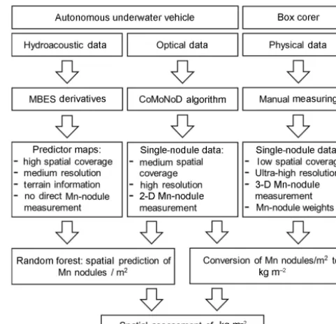
tistical techniques (e.g., kriging) in order to create quanti-tative maps of Mn-nodule abundance (Mucha et al., 2013; Rahn, 2017). However, the generally low number of ground-truth samples during surveys (usually below 10), their limited sampling area (typically 0.25 m2), and the relatively large distance between them (> 1 nm) prevent an accurate correla-tion with the ship-based MBES data and thus a good predic-tion of the total Mn nodules’ mass and distribupredic-tion in large areas (Petersen, 2017). Importantly, the sparse sampling with box corers affects the performance of interpolation and geo-statistical techniques, which are typically applied during data analysis (Li and Heap, 2011, 2014; Kuhn et al., 2016). In this article, we address this challenge by combining high-resolution hydroacoustic and optical data sets acquired with an autonomous underwater vehicle (AUV) and connecting those data with a machine learning (ML) algorithm (here ran-dom forests), in order to predict the spatial distribution of the number of Mn nodules per square meter. Unlike geostatisti-cal methods, ML can be used to incorporate information from different bathymetric derivative layers and to detect complex relationships among predictor variables without making any prior assumptions about the type of their relationship or value distribution (Garzn et al., 2006; Lary et al., 2016). To this end, first predictions have already been achieved (Knobloch et al., 2017; Vishnu et al., 2017; Alevizos et al., 2018). Here, we present a complete data analysis workflow for potential mining exploration (Fig. 1).

1.1 AUV hydroacoustic mapping

AUVs have proven their usefulness for multibeam data ac-quisition in the deep-sea environment (Grasmueck et al., 2006; Deschamps et al., 2007; Haase et al., 2009; Wynn et al., 2014; Clague et al., 2014, 2018; Pierdomenico et al., 2015; Peukert et al., 2018a). They achieve higher spatial and vertical resolution compared to ship-mounted MBESs. This is due to their operation close to the seafloor, which results in a smaller footprint at a given beam angle and enables the use of higher frequencies (Henthorn et al., 2006; Mayer, 2006; Caress et al., 2008; Paduan et al., 2009). Additionally, AUVs avoid problems like near-surface turbulences, bubbles,

Figure 1.Schematic workflow of the data sets used in this study to enable the spatial assessment of Mn nodules inside the study area. The medium resolution of AUV MBES (meter scale) refers to the comparison of the optical and physical data (centimeter scale).

ship noise, and strong sound velocity changes (Kleinrock et al., 1992a, b; Jakobson et al., 2016; Paul et al., 2016). They work independently from the surface vessel and op-erate at a stable altitude. AUVs can efficiently conduct a dive pattern of dense survey lines and thus reduce survey ef-fort and costs (Chance et al., 2000; Bellingham, 2001; Bing-ham et al., 2002; Danson, 2003; Roman and Mather, 2010). High-resolution bathymetry enables computing bathymetric derivatives like slope and rugosity with a similarly high res-olution. These derivatives play an important role in predict-ing Mn nodules’ distribution and abundance (Craig, 1979; Kodagali, 1988; Skornyakova and Murdmaa, 1992; Kodagali and Sudhakar, 1993, Sharma and Kodagali, 1993; Ko et al., 2006). However, a small number of recent studies have inves-tigated this role on an AUV scale (Okazaki and Tsune, 2013; Peukert et al., 2018a; Alevizos et al., 2018).

1.2 Underwater optical data

in the spatial distribution of nodules at meter scale. Thus optical data can fill the investigation gap between ground-truth sampling and hydroacoustic remote sensing (Sharma et al., 2010, 2013; Schoening et al., 2012a, 2014, 2015, 2016, 2017a; Kuhn and Rathke, 2017). Moreover, mosaicking of optical data could reveal mining obstacles such as outcrop-ping basements or volcanic pillow lava flows. In addition, seafloor photos are the source for evaluating benthic fauna occurrences and related habitats on a wider area (Schoening et al., 2012b; Durden et al., 2016).

1.3 Box corer sampling

Box coring is common to obtain physical samples of Mn nod-ules and sediments for resource assessments and biological studies. While optical data reveal only the exposed and semi-buried Mn nodules, box corers collect the top 30–50 cm of the seafloor with minimum disturbance, allowing an accu-rate measure of the Mn nodules’ abundance (kg m−2). Box coring data are used for training and validation in geostatis-tical methods for quantitative and spatial predictions of Mn nodules (e.g., Mucha et al., 2013; Knobloch et al., 2017). The representativeness of box coring data is disputable as few de-ployments can be made due to time constraints (ca. 4 h per core) and as the spatial coverage of one sample is rather low (ca. 0.25 m2).

1.4 Random forests

Random forests (RF) is an ensemble machine learning (ML) method composed of multiple weaker learners, namely clas-sification or regression trees (Breiman, 2001a). Within RF an ensemble of distinct tree models is trained using a random subsample of the training data for each tree until a maximum tree size is reached. In each tree, each node is split using the best among a subset of predictors randomly chosen at that node instead of using the best split among all variables (Liaw and Wiener, 2002). Thus, the process is double-randomized which further reduces the correlation between trees. About two-thirds of the training data are used to tune the RF while the remaining “out-of-bag” (OOB) samples are used for an internal validation. By aggregating the predictions of all trees (majority votes for classification, the average for regression), new values can be predicted. This aggregation keeps the bias low while it reduces the variance, resulting in a more pow-erful and accurate model. RFs have the ability to estimate the importance of each predictor variable, which enables data mining of the high-dimensional prediction data. Ter-restrial studies use RFs in prospectivity mapping of mineral deposits (Carranza and Laborte, 2015a, b; 2016; Rodriguez-Galiano et al., 2014, 2015). In the marine environment, RFs have been used to combine MBES bathymetry, backscatter, their derivatives, sediment sampling, and optical data for var-ious seabed classification and regression tasks (e.g., Li et al., 2010, 2011a; Che Hasan et al., 2014; Huang et al., 2014).

Further studies showed the robustness of RFs for selected data sets compared to other ML algorithms (Che Hasan et al., 2012; Stephens and Diesing, 2014; Diesing and Stephens, 2015; Herkul et al. 2017), as well as to geostatistical and de-terministic interpolation methods (Li et al., 2010, 2011a, b; Diesing et al., 2014).

2 Study area

The study area lies in the Clarion–Clipperton Zone (CCZ; ca. 4×106km2) in the eastern central Pacific Ocean. The CCZ has triggered scientific and industrial interest for sev-eral decades due to its high resource potential in Mn-nodule deposits (Hein et al., 2013; Petersen et. al., 2016) with an average nodule abundance of 15 kg m−2(SPC, 2013). At the time of writing, the International Seabed Authority (ISA) has granted 17 exploration licences inside the CCZ (Fig. 2a). The study area described here is part of the Belgian GSR (Global Sea Mineral Resources) license area (Fig. 2b) and will be referred to as block G77 (Fig. 2c). Overall, this part of the Belgian license area has a high bathymetric range and com-plex morphology, due to the presence of submarine volca-noes, solitary seamounts, and seamount chains. Block G77 is characterized by a low bathymetric range (77 m) and mostly gentle slopes (95 % of the area below 5◦). An exception is located in the eastern part, where subrecent small-scale vol-canic activity created 15 cone-shaped morphological features of up to 55 m height and 150 m width that are clustered in an area of ca. 700 m×380 m. Despite the gentle slopes, block G77 is characterized by an uneven microrelief (according to Dikau, 1990) especially in the western part, where small (2– 4 m) depressions coexist next to short (2–4 m) protrusions. In the central part, a 30 m high elevation acts as a natural barrier between the western part of the study area that features more relief and the eastern part that is deeper and has less relief (Fig. 2c).

3 Methodology

Figure 2. (a)Areas of Particular Environmental Interest (APEIs), licensed areas (white), and the Belgium/GSR licenses area (black) within the CCZ.(b)Regional bathymetric map of the study area, created by the EM 122 MBES on R/VSonne(cruise SO239).(c)Block G77, mapped by AUVAbysswith a Teledyne Reson Seabat 7125 MBES.

was conducted with the Teledyne PDS2000 software for data conversion of the raw data into s7k and GSF format. Further multibeam processing (sound velocity calibration, pitch/roll/yaw/latency artifacts correction) was performed using the Qimera™software. The largest uncertainties during AUV operations result from inaccurate navigation and local-ization in the deep-sea environment (Paull et al., 2014). AUV Abysshas a combination of five different systems for naviga-tion and posinaviga-tioning: Global Posinaviga-tioning System (GPS) when at the sea surface, Doppler velocity log (DVL) when 100 m or less from the ground, inertial navigation system (INS), long baseline acoustic navigation (LBL), and dead reckon-ing (GEOMAR, 2016). Each system has its own limitations that contribute to the total navigation error (Sibenac et al., 2004; Chen et al., 2013) that generally results in position-ing drifts over time. Consequently, this affects the position accuracy of the MBES and optical data. Our AUV MBES data processing and an absolute geo-referencing of the result-ing AUV bathymetry grid with the EM122 ship data, supple-mented with the use of MBnavadjust in MB-Systems (Caress et al., 2017), resulted in a well-calibrated AUV bathymetric data set. The position of the AUV image data “only” relies on the abovementioned sensors with a “small” position error

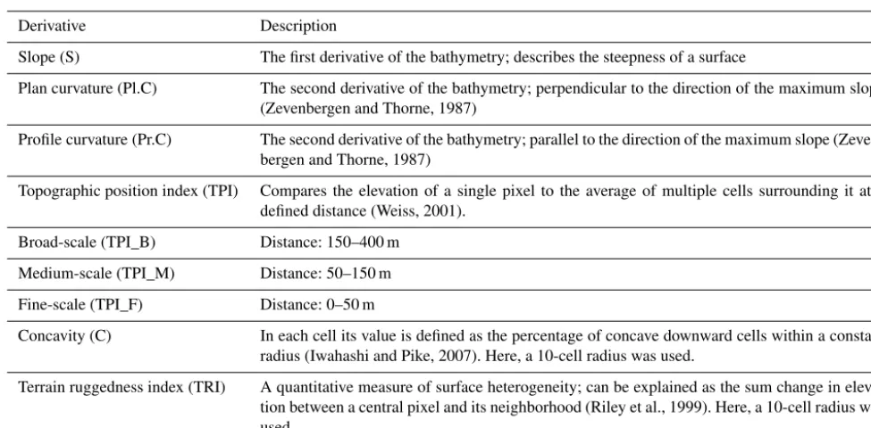
that is not quantifiable. Backscatter data were excluded from the modeling procedure due to artifacts and a generally poor quality. The output grid cell size for the analyses was set to 3 m×3 m. The depth raster was exported as ASCII format for further analysis in SAGA GIS v.6.3.0. SAGA includes numerous tools that focus on terrain analysis (Conrad, 2015). Eight bathymetric derivatives were computed (Table 1) with the SAGA algorithms (Appendix A).

me-Table 1.The bathymetric derivatives computed in SAGA GIS and used as predictor variables.

Derivative Description

Slope (S) The first derivative of the bathymetry; describes the steepness of a surface

Plan curvature (Pl.C) The second derivative of the bathymetry; perpendicular to the direction of the maximum slope (Zevenbergen and Thorne, 1987)

Profile curvature (Pr.C) The second derivative of the bathymetry; parallel to the direction of the maximum slope (Zeven-bergen and Thorne, 1987)

Topographic position index (TPI) Compares the elevation of a single pixel to the average of multiple cells surrounding it at a defined distance (Weiss, 2001).

Broad-scale (TPI_B) Distance: 150–400 m Medium-scale (TPI_M) Distance: 50–150 m Fine-scale (TPI_F) Distance: 0–50 m

Concavity (C) In each cell its value is defined as the percentage of concave downward cells within a constant radius (Iwahashi and Pike, 2007). Here, a 10-cell radius was used.

Terrain ruggedness index (TRI) A quantitative measure of surface heterogeneity; can be explained as the sum change in eleva-tion between a central pixel and its neighborhood (Riley et al., 1999). Here, a 10-cell radius was used.

ter (Mn nodules m−2), the nodule coverage of the seafloor in percent, and the nodule size distribution in square-centimeter size quantiles. The algorithm has successfully been applied for quantitative assessment and predictive modeling of Mn nodules (Peukert et al., 2018a; Alevizos et al., 2018). Nev-ertheless, the derived number of Mn nodules m−2is subject to uncertainties due to the limitations of the CoMoNoD al-gorithm and the nonconstant altitude of the AUV, especially in areas with slopes. The CoMoNoD algorithm cannot de-tect sediment-covered Mn nodules due to the low or nonex-istent contrast. It may count two or more adjacent small Mn nodules as one big nodule or misinterpret benthic fauna or rock fragments with similar visual features as Mn nodules. The CoMoNoD algorithm fits an ellipsoid around each de-tected Mn nodule, which limits the first two disadvantages as it splits huge Mn nodules and accounts for potentially buried parts (see discussions in Schoening et al., 2017a). In general, the first two disadvantages lead to underestimations while the third one results in an overestimation of the number of Mn nodules per square meter. These limitations are common, and the need for corrections (e.g., a factor that describes the ratio between the number of Mn nodules seen in the photo and the number of nodules counted in box corers, consider-ing for the different spatial scales) has been acknowledged (Sharma and Kodagali, 1993; Sharma et al., 2010, 2013; Tsune and Okazaki, 2014; Kuhn and Rathke, 2017). Recent studies show that the difference between image estimates and the abundance in box corer data (due to sediment covered Mn nodules) can be 2–4 times higher (Kuhn and Rathke, 2017). In this study, none of the box corers was obtained exactly at a location for which optical data exist; thus, no direct

com-parison and verification exist. Taking box corer samples for verification requires ultrashort baseline (USBL) navigation and imaging of the seafloor prior to the physical sampling. The effects of the nonconstant flying altitude on the detec-tion of Mn nodules per square meter are explained in detail below. For each photo location, the depth and the bathymet-ric derivative values were extracted from the hydroacoustic data. As no absolute geo-referencing could be performed for the AUV-based photo surveys, drifting sensor data will have an effect on the alignment between bathymetric and photo information, which was considered while interpreting the re-sults.

3.3 Data exploration and spatial analysis

im-and purposes during the cruise. Nevertheless, all box core samples (maximum distance < 1.5 km) were analyzed and used for further analyses. In the three box corers, the number, size, and weight of nodules were measured and the abun-dance (kg m−2) was estimated (mean value: 26.5 kg m−2). The total number of Mn nodules within each box corer was compared with the number of Mn nodules on the surface re-sulting in an average ratio of 1.32 (Table 2). This means that

≈25 % of the nodules are not seen on the surface but are completely buried within the sediment (down to a depth of about 15 cm).

3.5 RF predictive modeling

The RF modeling was performed with the Marine Geospatial Ecology Tools (MGET) toolbox in ArcMap™ 10.1. MGET (Roberts et al., 2010) uses the randomForests R package for classification and regression (Liaw and Wiener, 2002). Our target variable (number of Mn nodules m−2_{) is continuous,} so regression was applied. We followed the three main steps to establish a good model by selecting predictor variables, and calibration/training of the model and finally validating the model results.

Selection of predictor variables. The depth (D) and its derivatives (Table 1) were used as predictor variables. Al-though RFs can handle a high number of predictor vari-ables with similar information, the exclusion of highly cor-related variables can improve the RF performance and de-crease computation time (Che Hasan, 2014; Li et al., 2016). Thus, the correlation between derivatives was investigated using the Spearman’s rank correlation coefficient. None of the variable pairs was perfectly correlated (ρ≥95), and con-sequently, all of them were used for RF modeling (Ap-pendix A).

Calibration of the model. During the calibration process, the RF parameters were adjusted as follows. The number of predictor variables to be randomly selected at each node (mtry), the minimum size of the terminal nodes (nodesize), and the number of trees to grow (ntree) were set to the default values, in order to investigate the optimum training size. For regression RF the defaultmtryvalue is 1/3 of the number of

raw variable importance was preferred (unscaled) as the fi-nal parameter (Diaz-Uriarte and de Andres, 2006; Strobl et al., 2008, 2009; Strobl and and Zeileis, 2008). Using these settings, the influence of the training sample size was exam-ined (10 % to 90 % of the total sample in steps of 10 %) and compared based on the mean of squared residuals (MSR) us-ing the respective equation provided in the randomForests R package (Liaw and Wiener, 2002). The different training groups need to be considered as representative of the total sample, in order to capture the heterogeneity of the Mn nod-ules’ spatial distribution. The spatially random selection of subsamples by MGET ensured similar statistical character-istics in each group (Appendix A). For each case of differ-ent training sample size, the model was run 10 times and the results are presented as the average value of these 10 runs (Appendix B). Since the optimal training sample size was defined, the influence of the number of growing trees (ntree) and the influence of the number of predictor variables to be randomly selected at each node (mtry) was examined. Only for the already defined optimum training size were 10 dif-ferentntreevalues (100 to 1000 in steps of 100) and seven differentmtryvalues (1 to 7 in steps of 1) tested and com-pared based on the MSR values. In each case of a different ntreeandmtryparameter, the model was run 10 times, and the results are presented as the average value of these 10 runs (Appendix B).

Table 2.The number of Mn nodules on the sediment surface, the total number of Mn nodules per box core, the ratio of those two values, and the distance of the box corer deployments from the study area in block G77.

Box corer Total number Number of Mn nodules Ratio Abundance Distance from station of Mn nodules at the surface (kg m−2) G77 area (km)

BC20 40 27 1.5 – 0

BC21 67 58 1.1 27.1 1.4

BC22 29 21 1.4 27.1 0.6

BC23 32 20 1.6 25.2 0.1

BC24 17 16 1.0 – 1

Average 37 28 1.32 26.5 0.6

should not be used solely as an index for the model per-formance (Willmott and Matsuura, 2005). Both MAE and RMSE are measured in the same unit as the data. In addition, theR2, Pearson (r), and Spearman’s rank correlation coeffi-cients were used to identify the correlation between predicted and initial values. Finally, the descriptive statistics of pre-dicted and initial values were compared and a residual anal-ysis was performed.

3.6 Resource assessment

As the optimal RF model was applied to the entire block G77, an estimate of the abundance (kg m−2) was computed, based on the analogy between the corresponding abundance mea-sured from the average number of Mn nodules in the box corer data and the number of Mn nodules m−2in each cell of the final result of the RF model. Considering that the collec-tor can recover buried Mn nodules from a maximum depth of 10–15 cm (Sharma, 1993, 2010), the ratio of 1.32 was ap-plied to account for Mn nodules not detected in the images, and areas with a slope of > 3◦were excluded, assuming that a potential mining vehicle is limited to less steep slopes (UN-OET, 1987).

4 Results

4.1 Data exploration

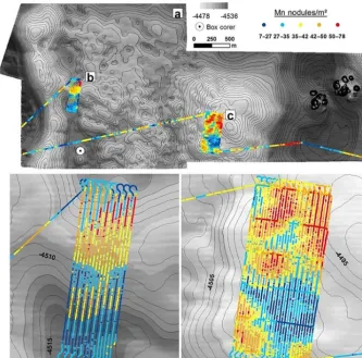
The analysis of AUV photos with the CoMoNoD algorithm (Schoening et al., 2017a) revealed a rather heterogeneous pattern of Mn nodules m−2 in the study area, showing ad-jacent areas with high and low Mn-nodule number (Fig. 3a). The number of Mn nodules m−2 changes within less than 100 m in the overall study area and in the two main subareas b and c (Fig. 3a–c). In half of the photos (48 %), the number of Mn nodules m−2varies from 30 to 43 with the mean value being 36.6 Mn nodules m−2. The very small change of 5 % trimmed mean value indicates the absence of extreme out-liers, which is confirmed by box plot analysis (Appendix B). Further analysis of their descriptive and distribution char-acteristics was performed in order to assess the presence of normality in the data, with the result that the number of

Mn nodules m−2_{is approximately normally distributed} (Ap-pendix B). Although the presence of normality in data is not a prerequisite assumption in order to perform the RF (Breiman, 2001a), as it is with geostatistical interpolation techniques like kriging (e.g., Kuhn et al., 2016), this examination can give us a better understanding of the Mn nodules’ distribu-tion inside the study area, and it is an important step in order to examine potential extreme observations which may be de-rived from wrong measurements and could artificially change the training range during RF predictive modeling. Moreover, an absence of linear correlation was observed between Mn nodules m−2and the produced bathymetric derivatives, indi-cating the complexity of the phenomenon (Appendix B).

4.2 Spatial analyses

Spatial analyses revealed the presence of a spatial autocor-relation in the distribution of Mn nodules m−2. The GMI, withI =0.6989,p<0.01, and a Z score > 2.58 indicates a positive spatial autocorrelation. According to the incremen-tal analysis, the index takes its highest value in the first 50 m with a gradual decrease, approaching 0 values after a dis-tance of 400 m (Fig. 4a). Similarly, the results from the LMI show that the main size of the spatial clusters does not ex-ceed 400 m in either direction (Fig. 5a). The main types of these clusters are H–H and L–L groups (Fig. 4b and Table 3). A distinct “buffer/transitional zone” with Mn nodules was found between these two clusters, which does not show a sig-nificant autocorrelation (Fig. 5b, c). Approximately one-third of the data does not have a significant clustering (NS). In the subarea c, the few local H–L and L–H groups are located in the outer parts of these zones without significant spatial clustering. Both H–L and L–H (from the entire study area) only account for 2.1 % of the data (Table 3). The compari-son of the number of Mn nodules m−2 _{between the groups} shows a clear discrimination between H–H and L–L clusters (Fig. 5b). The H–H clusters are in areas with 37.9–78.2 Mn nodules m−2 whilst the L–L clusters are in areas with 6.8– 35.2 Mn nodules m−2.

Figure 3. (a)The spatial distribution of Mn nodules m−2inside block G77 and the box corer position.(b)The spatial distribution of Mn nodules m−2inside the subarea b.(c)The spatial distribution of Mn nodules m−2inside the subarea c.

Figure 4. (a)The GMI decrement due to increasing distance, after the first 50 m.(b)The range of Mn nodules m−2in each clustered group.

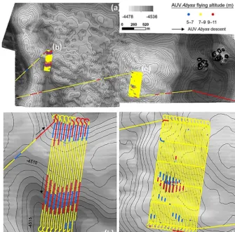
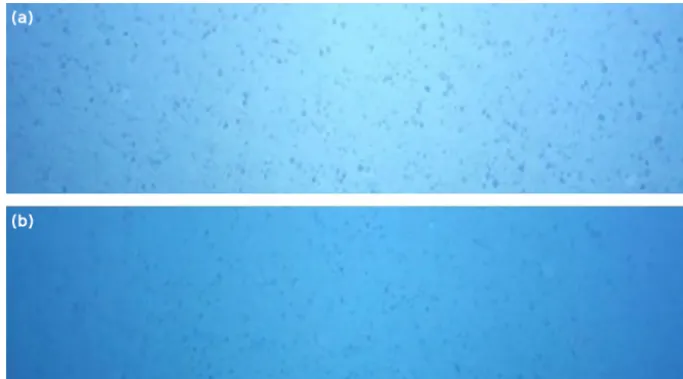
the AUV to vary its altitude between the ascending and de-scending phase (Fig. 6b). This variation seems to affect the image quality, resulting in fewer nodules being counted for higher altitudes of the AUV (Figs. 7 and 8). This is also

Figure 5. (a)The spatial distribution of the significant cluster types inside the block G77.(b)The spatial clusters inside the subarea b.(c)The spatial clusters inside the subarea(c).

Table 3.Number and percentage of samples in each type of spatial clustering.

Cluster type H–H H–L L–H L–L NS Counts (n) 3472 121 113 3523 4047 Counts (%) 30.8 1.1 1.0 31.2 35.9

scale can hide this bias during plotting. The comparison of the detected Mn nodules m−2in these adjacent lines, inside the small subarea b, gives a ratio≈1.4 between photos that have been acquired at 7–9 m altitude and those at 9–11 m al-titude. The ratio is higher (≈1.8) between photos from 5– 7 and 9–11 m altitude. In contrast, the ratio between photos from 5–7 m altitude and those at 7–9 m altitude is≈1.25, in-dicating that the problem mainly exists at upper and lower flying altitudes. Despite their different ratio, none of these groups contain extremely high or low values of Mn nodules m−2. Moreover, in several parts of the block, the photos from higher altitude are the only source of information without the ability for further comparison, and consequently, they cannot be excluded from the modeling procedure.

Spatial distribution of median size. Plotting of the median size in square centimeters (Fig. 9) showed that the number of Mn nodules m−2_{is anti-correlated to the median Mn-nodule} size. The Spearman’s rank correlation coefficient andR2 be-tween these two variables are−0.50 and 0.25, respectively, supporting this observation (Fig. 10a); other studies found similar results (Okazaki and Tsune, 2013; Kuhn and Rathke, 2017; Peukert et al., 2018a). The box plot analysis of the me-dian size values between the H–H and L–L clustered groups showed that although the L–L group contains the entire range of median size values (2.8 to 15.9 cm2), the H–H group does not contain values above 10 cm2 (2.7–10 cm2). This means in consequence that in areas with significant clustering of higher numbers of Mn nodules m2, the size of Mn nodules tends to be smaller (Fig. 10b).

4.3 RF predictive modeling

4.3.1 Effect of training sample size andntreeandmtry parameters

Figure 6. (a)The altitude of AUVAbyssinside block G77.(b)The altitude inside the small subarea b, where the presence of the slope forces the AUV to modify its altitude, flying closer to the seafloor in the ascending phase (blue lines) and farther from the seafloor in the descending phase (red lines).(c)In the big subarea c, the AUV flying altitude is mainly constant between 7–9 m for the entire part.

Figure 7. Scatterplot of the AUV altitude (m) and the estimated number of Mn nodules m−2inside subarea b. The colors correspond to the color scale in Fig. 7.

(Fig. 11a). This finding is in accordance with other studies, in which larger training samples tended to increase the

en-Figure 8.Adjacent AUV photos from consecutive dive tracks that were obtained inside subarea b from(a)lower (5–7 m) and(b)higher (9–11 m) altitudes. Note the decrement in the image brightness. (The area of the photos represents the central part of the photo, i.e., ca. 1/4 of the original photo size.)

Figure 10. (a)The plot of median size (cm2) and number of Mn nodules m−2.(b)The range of median size (cm2) in each type of cluster. Note the distinct difference in the range between the H–H and L–L cluster type.

ables highermtryvalues as there are more opportunities for each variable to occur in several trees (Strobl et al., 2009). Similarly to thentreeparameter, a larger number ofmtry val-ues results in a reduced error (Fig. 11c). The error reaches a minimum and cannot be reduced further for mtry=6; with values below 3, the error increases significantly. The differ-ent numbers of ntree reduced the error by only 0.6 in the MSR (from 18.8 to 18.2); in contrast, different mtryvalues reduced the error by 5.8 in the MSR (23.4 to 17.6), high-lighting its importance for the prediction accuracy. In gen-eral a higher number ofmtryvalues is suggested for RF stud-ies with correlated variables to result in a less biased result regarding the importance of each variable; this is because the higher number increases the competition between highly correlated variables, giving more chances for different selec-tions (Strobl et al., 2008). The finally selectedmtryvalue of 6 coincides with the recommended approach for mtry (de-fault, half of the de(de-fault, and twice the default) suggested by Breiman (2001a). Despite the importance of this analysis, within the model with 80 % of the data as a training sample, the decrease in error by the use of RF tuned values instead of RF default values was only 0.7 in the MSR values, whilst the greatest reduction in error (16.5 in the MSR values) came from the increase in training data set size. This highlights the increased sensitivity of the method with respect to training data and that the recommended settings in the R randomFor-est package (Lia and Wiener, 2002) give trustworthy results, increasing its simplicity and operational character.

4.3.2 Selection, application and external validation of the optimal model

Based on the abovementioned findings, the optimal RF re-gression model, which uses 80 % of training data, 600 trees, and 6 predictor variables to be randomly selected at each node, was selected and applied to the entire block G77. The

Table 4.The values of validation measures between predicted and observed data.

MAE MSE RMSE R2 Pearson Spearman 3.1 19.0 4.4 0.8 0.9 0.9

comparison of the predicted values with the observed values from the remaining 20 % (2255 observations) of validation data showed a good predictive performance (Table 4). Ana-lytically, MAE and RMSE have very low values,R2has a high value, and both Pearson’s and Spearman’s correlation coefficients show a strong positive correlation between the predicted and observed values. The small deviation between MAE and RMSE and the same good correlation of the Pear-son and Spearman factor point towards the absence of ex-tremely high or low predicted values (outliers). Moreover, the performance is rather stable among all the iterations (Ap-pendix B).

The scatterplot and box plot (Fig. 12a and b) illustrate this good match between predicted and observed values, as con-firmed also by the descriptive statistics (Table 5). The resid-ual analysis confirmed further the robustness of the model (Appendix B).

Figure 11. (a)The effect of training sample size in RF error (in MSR).(b)The effect of thentreeparameter in RF error (in MSR) for the 80 % training size.(c)The effect of themtryparameter in RF error (in MSR) for the 80 % training size.

Figure 12.Comparison between observed and predicted values: scatterplot(a)and box plots(b).

4.3.3 RF-predicted distribution of Mn nodules m−2 The final application of the RF model for the entire block G77 predicts that the majority of the area is covered by 30– 45 Mn nodules m−2(Fig. 13). In the central western part the distribution is quite uniform (at this scale) with few small ar-eas of lower numbers. In the western part, there are two ex-tended areas along the base of the hill with the lowest num-ber of Mn nodules m−2. Both of these areas have a linear shape in N–S direction and follow the seafloor topography with increased slope (> 3◦_{). The third main patch with} mini-mum Mn nodules m−2_{occurs in the eastern depression part.} In contrast, areas with a higher number of Mn nodules m−2 are located mainly in the central upper part of the hill and eastward facing slope of eastern depression and south of the subrecent hydrothermally active area.

4.3.4 RF importance

The analysis of the RF variable importance showed that the best explanatory variable for the distribution of Mn nod-ules m−2 is depth (Fig. 14a). The partial dependence plot

Figure 13.The RF-predicted distribution of Mn nodules m−2inside block G77.

values were selected based on the minimum possible corre-lation among them.

4.3.5 Estimation of abundance (kg m−2_{) of Mn nodules} The predicted Mn-nodule distribution was combined with the abundance from box corer data (and corrected with the ratio of buried to unburied Mn nodules, in order to include the top

∼15 cm of the sediment), resulting in the Mn nodules’ abun-dance map shown in Fig. 15. According to this map, block G77 is a promising area for mining operations. The entire block is above the cutoff abundance of 5 kg m−2 (UNOET, 1987), with a mean value of 33.8 kg m−2. We calculated that 84 % of block G77 has slopes below 3◦; steeper slopes are lo-cated mainly at the outer parts of the block, a fact that would ease establishing an ideal mining path. In this respect, the AUV scale mapping provides vital information for a poten-tial mining path by decreasing the possibility of machine fail-ure due to poorly mapped steep slopes not detected by, e.g., ship-based bathymetry (Peukert et al., 2018b). Mn-nodule distribution maps with this resolution increase the mining ef-ficiency because local deposit variations can significantly af-fect the performance of the pickup rate, which is likely deter-mined by technical parameters of the mining vehicle as well as the size, burial depth, and abundance of Mn nodules in the seafloor (Chung, 1996). The exclusion of areas with slopes > 3◦resulted in 8 km2minable seafloor surface. Assuming a constant 80 % collection efficiency (Volkmann and Lehnen, 2018) and a 30 % reduction in the Mn-nodule weight by the removal of water (Das and Anand, 2017), the dry mass of

Table 6.The estimated amount of metal mass for five metals, based on the average values of metal content inside CCZ and a five-metal HCL-leach recovery method (Volkmann, 2015).

Total wet mass (t): 270 400 Total dry mass (t): 189,280

Metal content Mn Ni Cu Co Mo Wt % 26.68 1.31 1.11 0.22 0.06 Equal to (t) 50 500 2480 2101 416 113 90 % metal 45 450 2232 1891 374 102 recovery (t)

Mn nodules that can be extracted from the surface and the first 15 cm of the sediment column amounts to ca. 190 000 t. In a back-of-the-envelope calculation this quantity – assum-ing constant metal content inside the study area, equal to the average metal concentrations inside the CCZ (Table 6) (Volk-mann, 2015), and 90 % metal recovery efficiency – could re-sult in an estimated resource haul of 45 450 t Mn, 2232 t Ni, 1891 t Cu, 374 t Co, and 102 t Mo (Table 6).

5 Discussion

Figure 14. (a)The variable importance of each predictor in the RF model.(b)The partial dependence plot of depth. The ticks on the graphs indicate the deciles of the data.

Figure 15.The total abundance of Mn nodules from the surface and embedded in the sediment (max 15 cm), in areas with slope≤3◦inside block G77 (continuous values of abundance are not given due to confidentiality).

data in areas of scientific and commercial interest can pro-vide more precise bathymetric and Mn-nodule distribution maps. Regarding the bathymetric maps, the accurate and de-tailed reconstruction of the seafloor bathymetry at meter-scale resolution enables to use bathymetry and its deriva-tives as source data layers within a high-resolution RF model. These data should have high-quality characteristics, as the presence of acquisition artefacts may affect the robustness of the modeling procedure (Preston, 2009; Herkül et al., 2017). The combined use of cameras as the DeepSurveyCamera (Kwasnitschka et al., 2016) for acquiring high-resolution photographs and an automated analysis with a state-of-the-art algorithm (Schoening et al., 2017a) provide essential quantitative information about the distribution of Mn nod-ules. Image analysis results are more robust for constant AUV altitudes (7–9 m) above flat areas (< 3◦), while the al-ternation of the flying altitude and camera orientation during the ascending and descending phases limits the quality of the

obtained images and can affect the derived number of Mn nodules m−2.

re-teristics of the seafloor affects the sediment deposition en-vironment and bottom currents and thus also geochemical processes in the sediment. All these factors determine Mn-nodule growth and thus affect the distribution of Mn Mn-nodules on regional scales (e.g., Craig, 1979; Sharma and Kodagali, 1993). It is still unknown how these properties influence the Mn-nodule distribution on meter to tens of meter scales as seen in our AUV data. The nonlinear relationship between Mn nodules and bathymetry on such high-resolution scales only began to be investigated very recently (e.g., Peukert et al., 2018; Alevizos et al., 2018). To elaborate more on the hydrodynamic and geochemical reasons behind the observed distribution pattern, we would need more investigations at and in the sediment on the same scale.

It should be acknowledged that the aim of any ML pre-dictive model is to derive accurate predictions based on an existing (large) number of measurements to capture a com-plex underlying relationship (e.g., nonlinear and multivari-ate) between different types of data, for which our theoreti-cal knowledge or conceptual understanding is still under de-velopment (Schmueli, 2010; Lary et al., 2016). Especially due to the constantly increasing size of scientific multivari-ate data in marine sciences and the existence of such non-linear relationships between predictor and response variables (e.g., Zhi et al., 2014; Li et al., 2017), ML and RF are con-sidered important analytic tools that can objectively reveal patterns of a (unknown) phenomenon (Genuer et al., 2017; Kavenski et al., 2009; Lary et al., 2016). Such predictions may be used to derive causalities or may drive the creation of new hypotheses. In other words, for a predictive model, the “unguided” data analyses come first and the interpreta-tion follows (Breiman, 2001b; Schmueli, 2010; Obermeyer and Emanuel, 2016). This “a priori” knowledge of the dis-tribution of the Mn-nodule number and size on such a scale can contribute to the biological data survey planning, too. Recent studies showed that the abundance and species rich-ness of nodule fauna inside the CCZ is affected by the abun-dance of Mn nodules (Amon et al., 2016; Vanreusel et al., 2016) as well as their size (Veillette et al., 2007). Thus, high-priority areas (e.g., those with the highest commercial in-terest) can be targeted for sampling based on the results of

RF has a high operational character due to its relatively sim-ple calibration, which does not request extensive data prepa-ration/transformation or the need for geostatistical assump-tions (e.g., stationarity). The selection of the MGET toolbox (Roberts et al., 2010) further increased the simplicity of the workflow, as the RF modeling was performed entirely in-side a graphic environment familiar to many geoscientists. As RF model runs can be implemented inside various soft-ware packages in future implementations of this workflow, it would be interesting to include the uncertainty for the asso-ciated predictions, e.g., with the use of the quantile regres-sion forests (Meinshausen, 2006) from the quantregForest R package (Meinshausen, 2012). However, this will increase the computational time (Tung et al., 2014) and the simplic-ity of the procedure, especially if other recently proposed methodologies of estimating the uncertainty are used: the jackknife method (Wager et al., 2014), the Monte Carlo ap-proach (Coulston et al., 2016), and theUstatistics approach (Mentch and Hooker, 2016).

entire range of the number of Mn nodules m−2 and come from all the different sub-terrains), would most likely rein-force the model to build better and wider relationships be-tween the predictor and response variables, keeping also a larger number of validation data points.

Finally, the resource assessment showed that block G77 is a potential mining area with high average Mn-nodule density and gentle slopes. While the threshold of 3◦(UNOET, 1987) was used here, newer plans for mining machines seem to en-able operations on steeper slopes (Atmanand and Ramadass, 2017), increasing the total amount of collected Mn nodules within the area considered herein.

6 Conclusions

The results of this study show that the acquisition and anal-ysis of optical seafloor data can provide quantitative infor-mation on the distribution of Mn nodules. This inforinfor-mation can be combined with AUV-based MBES data using RF ma-chine learning to compute predictions of Mn-nodule occur-rence on small operational scales. Linking such spatial pre-dictions with sampling-based physical Mn-nodule data pro-vides an efficient and effective tool for mapping Mn-nodule abundance.

distributed among the features in the study area. For the op-timal conceptualization of spatial relationships, the inverse Euclidian distance method was selected, as it is appropriate for modeling processes with continuous data in which the closer two samples are in space, the more likely they are to interact/influence each other or have been influenced for the same reasons. The distance threshold was set at 50 m, and the increment analysis was performed with a step of 50 m. Moreover, the spatial weights were standardized in order to minimize any bias that exists due to sampling design (un-even number of neighbors). Apart from the index value, thep value andZscore are also provided. The local Moran’s I in-dicates statistically significant clusters and outliers for a 95 % confidence level. The high number of observations (30) that was used ensures the robustness of the indexes.

Table A1.Spearman’s correlation coefficient for each pair of predictor variables.

D S Pl.C Pr.C TPI_B TPI_M TPI_F C TRI

D

S −0.07

Pl.C 0.06 −0.02 Pr.C 0.08 −0.01 0.37 TPI_B 0.76 −0.09 0.13 0.16

TPI_M 0.36 −0.06 0.20 0.27 0.72

TPI_F 0.23 −0.05 0.33 0.41 0.47 0.77 C −0.30 0.05 −0.25 −0.34 −0.54 −0.79 −0.90 TRI −0.10 0.91 −0.02 −0.03 −0.12 −0.06 0.04 0.05

Table A2.Descriptive statistics of different training samples.

% training sample: 10 % 20 % 30 % 40 % 50 % 60 % 70 % 80 % 90 %

Training set size 1127 2255 3383 4511 5638 6766 7894 9021 10148 Mean 36.5 36.3 36.6 36.6 36.6 36.7 36.6 36.7 36.6 SE 0.3 0.2 0.2 0.1 0.1 0.1 0.1 0.1 0.1 SD 9.3 9.2 9.4 9.2 9.2 9.3 9.3 9.2 9.3

Minimum 7 13 12 13 12 14 7 7 7

Maximum 63 70 72 66 78 78 78 72 78

Appendix B: Results

B1 RF predictive modeling (calibration of the model) The descriptive statistics of the performance of each model were used as decision factors for the number of iterations (Tables B1–B5). In all cases, the mean value with very low standard error, very low standard deviation, range, and the 95 % confidence interval indicate a rather stable perfor-mance, without the need for further iterations.

B1.1 Data exploration

The histogram of Mn nodules m−2(Fig. B1) shows a good fit with the superimposed theoretical normal curve, with the shape of the distribution being rather symmetrical. This fact is supported by the equal 5 % trimmed mean and median and the slightly different mode (Table B6). Similarly, the visual inspection of the probability plot (Fig. B1) shows a good match as a linear pattern is observed for the greatest part, with slight deviation existing only in the outer parts of the curve. According to the box plot, there are only 21 mild outliers (according to Hoaglin et al., 1986; Dawson, 2011), which correspond to 0.18 % of the total observation. This percentage is smaller than the 0.8 % threshold that has been suggested for normal disturbed data (Dawson, 2011).The small values for skewness and kurtosis combined with the large sample size further support the normally distributed pattern of the data (Table B6). Especially for large data sam-ples, measurements of skewness and kurtosis combined with the visual inspection of histogram and probability plot are recommended ways of examining the normality (D’Agostino et al., 1990; Yaziki and Yolacan, 2007; Field, 2009; Ghasemi and Zahediasl, 2012; Kim, 2013).

The potential linear correlation between depth, bathymet-ric derivatives, and the number of Mn nodules m−2was in-vestigated using the Spearman’s rank correlation coefficient (ρ) (Table B7) because of the skewed distribution and pres-ence of extreme values in the depth and bathymetric deriva-tive values (Mukaka, 2012).

B1.2 Selection, application, and external validation of the optimal model

Despite the fact that RF is a full nonparametric technique and there is no need for the residuals to follow specific as-sumptions (Breiman, 2001a), the examination of them can provide an in-depth look at RF performance characteristics. The scatterplot of residuals against predicted values shows a random pattern, which is also confirmed by the low values of Pearson, Spearman, andR2coefficients between predicted values and residuals (Fig. B2 and Table B8). Moreover, the residuals tend to cluster towards the middle of the plot with-out being systematically high or low and having a zero mean value (Fig. B2 and Table B9). Their constant variance (ho-moscedasticity) implies that the distribution of error has the

same range for almost all fitted values. Indeed, 99.3 % of the residuals are inside the range±15 and 81.2 % are inside the range±5 (Table B10). The presence of outliers is very lim-ited without affecting the main statistical characteristics of residuals (Table B9), indicating that the model adequately fits the overwhelming majority of the observations (> 2165) and only random variation (that exists in any real, natural phenomenon) or noise can occur.

The spatial autocorrelation analysis of the residuals using the global Moran’s index (same settings as Appendix A), showed low spatial autocorrelation (I=0.112112,p<0.01 andZ score > 2.58). The index number of the residuals is relatively low compared with the high initial values of the original data (I =0.69890 andI =0.697747 for the entire data set and the 80 % training data set, respectively). More-over, the spatial autocorrelation of the 5 % trimmed residuals is only 0.093832. According to similar studies (i.e., regres-sion RF), the presence of spatial autocorrelation in the resid-uals of the model can result in underestimation of the true prediction error (Ruß und Kruse, 2010). The presence of low spatial autocorrelation values in the residuals of regression RF has been reported also by other authors (e.g., Mascaro et al., 2014; Xu et al., 2016), and it is a common problem in all the well-established machine learning methods (e.g., random forests, neural network, gradient boosting machines, and sup-port vector machines) when dealing with regression predic-tions of spatial variables (Gilardi and Bengio, 2009; Ruß und Kruse, 2010; Santibanez et al., 2015a, b). The spatial plotting and visual examination of the residuals (Fig. B3) showed that this spatial clustering exists mainly in the small subarea b and especially in the areas which are associated with an increased slope (>3◦_{), where the AUV is forced to vary its altitude} be-tween the ascending and descending phase and consequently affects the image quality and the later modeling results. B1.3 RF importance

Table B2. Descriptive statistics of MSR from a different number of thentree parameter, after 10 iterations with 80 % of the sample as training data andmtry=3.

ntree: 100 200 300 400 500 600 700 800 900 1000 Mean 18.8 18.4 18.3 18.3 18.3 18.2 18.2 18.2 18.2 18.2 SE 0.0 0.0 0.0 0.0 0.0 0.0 0.0 0.0 0.0 0.0 Median 18.8 18.4 18.3 18.3 18.3 18.2 18.2 18.2 18.2 18.2 Mode 18.8 18.4 18.3 18.3 18.3 18.2 18.2 18.2 18.2 18.2 SD 0.1 0.1 0.1 0.1 0.0 0.1 0.1 0.1 0.0 0.0 Minimum 18.5 18.4 18.2 18.2 18.2 18.1 18.1 18.1 18.1 18.1 Maximum 18.9 18.5 18.5 18.4 18.3 18.3 18.3 18.3 18.2 18.2 C.I. (95.0 %) 0.1 0.0 0.1 0.0 0.0 0.0 0.0 0.0 0.0 0.0

Table B3.Descriptive statistics of MSR from different number of themtryparameter, after 10 iterations with 80 % of the sample as training data andntree=600.

mtry: 1 2 3 4 5 6 7

Mean 23.4 19.3 18.2 17.9 17.7 17.6 17.6 SE 0.0 0.0 0.0 0.0 0.0 0.0 0.0 Median 23.4 19.3 18.2 17.9 17.7 17.6 17.6 Mode 23.4 19.3 18.2 17.9 17.7 17.6 17.6 SD 0.0 0.1 0.1 0.1 0.0 0.0 0.0 Minimum 23.3 19.1 18.1 17.8 17.6 17.5 17.6 Maximum 23.5 19.4 18.3 17.9 17.7 17.7 17.7 C.I. (95.0 %) 0.0 0.1 0.0 0.0 0.0 0.0 0.0

Table B4.Descriptive statistics of MSR for the optimum selected RF model, after 30 iterations with 80 % of the sample as training data,

ntree=600, andmtry=6.

Table B5.Descriptive statistics of RF importance for the optimum RF model, after 30 iterations with 80 % of the sample as training data,

ntree=600, andmtry=6.

RF importance: Depth TPI_B TPI_M TRI TPI_F C S Pl.C Pr.C Mean 80.1 63.6 46.7 36.1 24.5 19.7 12.0 2.6 2.4 SE 0.1 0.1 0.1 0.0 0.0 0.0 0.0 0.0 0.0 Median 80.1 63.5 46.7 36.1 19.7 19.7 11.9 2.6 2.4 Mode 80.1 63.3 46.9 36.1 19.8 19.8 11.9 2.6 2.4 SD 0.4 0.6 0.6 0.2 0.2 0.2 0.2 0.0 0.0 Minimum 79.1 62.6 45.0 35.7 19.2 19.2 11.7 2.5 2.3 Maximum 80.8 64.9 47.7 36.4 20.1 20.1 12.4 2.6 2.5 C.I. (95.0 %) 0.1 0.2 0.2 0.1 0.1 0.1 0.1 0.0 0.0

Figure B1. (a)Histogram of Mn nodules m−2with the superimposed normal curve.(b)The normal probability plot of Mn nodules m−2.(c)

The box plot of Mn nodules m−2.

Table B6.The descriptive statistics of the number of Mn nodules m−2.

Mean 5 % trim. mean Median Mode SD Min Max Skew. Kurtosis Mn nodules m−2 36.6 36.4 36.4 39 9.2 6.8 78.2 0.1 −0.4

Table B7.The Spearman’s rank correlation coefficient between Mn nodules m−2, depth, and bathymetric derivatives.

Figure B2.Scatterplot between residuals and predicted values.

Table B8.Pearson, Spearman, andR2correlation coefficients be-tween residuals and predicted values.

Pearson Spearman R2

Correlation of residuals and predicted values 0.1 0.2 0.0

Table B9.Main descriptive statistics of residuals and 5 % trimmed residuals.

Mean SE Median Mode SD Residuals −0.2 0.1 −0.2 0.6 4.4 5 % trimmed −0.2 0.1 −0.2 0.6 2.9 residuals

Table B10.Residuals range.

Author contributions. IZG processed the MBES and AUV data, performed the RF modeling, the statistical and GIS analysis, and wrote the paper. TS contributed to the survey design with respect to the optic data, developed the CoMoNoD algorithm, and processed the optic data. EA was involved in developing the idea of using RF for modeling and contributed to the GIS analysis. JG contributed to the survey by designing the MBES and the optic data survey plan-ning, acquiring the MBES and the optic data, verifying the analyti-cal methods, and supervising the project. All authors discussed the results, provided critical feedback, and contributed to the final pa-per.

Competing interests. The authors declare that they have no conflict of interest.

Special issue statement. This article is part of the special issue “Assessing environmental impacts of deep-sea mining – revisiting decade-old benthic disturbances in Pacific nodule areas”. It is not associated with a conference.

Acknowledgements. We thank the captain and crew of RVSonne

for their contribution to a successful cruise. We express our gratefulness to the GEOMAR AUV team for their support during the cruise. We thank Anja Steinführer for preprocessing of the AUV MBES data and Mareike Kampmeier for advice during the post-processing analysis of the MBES data. We thank Inken Preuss for proofreading the paper. Finally, we thank the GEOMAR Library team for its support in gathering the necessary bibliography. All data were acquired within the framework of the JPIO Project “Ecological Aspects of Deep-Sea Mining”, funded through BMBF grant 03F0707A. Funding for Iason-Zois Gazis was also made available through MarTERA grant COMPASS-Drimp from BMWi (03SX466B). This is publication 35 of the DeepSea Monitoring Group at GEOMAR Helmholtz Centre for Ocean Research Kiel. Edited by: Daniel O. B. Jones

Reviewed by: two anonymous referees

References

Alevizos, E., Schoening, T., Koeser, K., Snellen, M., and Greinert, J.: Quantification of the fine-scale distribution of Mn-nodules: insights from AUV multi-beam and optical imagery data fusion, Biogeosciences Discuss., https://doi.org/10.5194/bg-2018-60, in review, 2018.

Anselin, L.: Local Indicators of Spatial Association – LISA, Geogr. Anal., 27, 93–115, https://doi.org/10.1111/j.1538-4632.1995.tb00338.x, 1995.

Atmanand, M. A. and Ramadass, G. A.: Concepts of Deep-Sea Mining Technologies, in: Deep-Sea Mining, edited by: Sharma, R., Resource Springer, Cham. Online ISBN 978-3-319-52557-0, https://doi.org/10.1007/978-3-319-52557-0_6, 2017.

Bellingham, J.: Autonomous underwater vehicles (AUVs), in: Encyclopedia of Ocean Sciences, edited by:

Steele, H., Academic Press, San Diego, 212–216, https://doi.org/10.1006/rwos.2001.0303, 2001.

Bingham, D., Drake, T., Hill, A., and Lott, R.: The Application of Autonomous Underwater Vehicle (AUV) Technology in the Oil Industry – Vision and Experiences. FIG XXII International Congress Washington, DC USA, 19–26 April, 1–13, 2002. Breiman, L.: Random forests, Machine Learning, 45, 5–32,

https://doi.org/10.1023/A:101093340, 2001a.

Breiman, L.: Statistical Modeling: The Two Cultures, Stat. Sci., 16, 199–215, https://doi.org/10.1214/ss/1009213726, 2001b. Caress, D. W. and Chayes, D. N.: MB-System: Mapping

the Seafloor, available at: https://www.mbari.org/products/ research-software/mb-system (last access: 6 December 2018), 2017.

Caress, D. W., Thomas, H., Kirkwood, W. J., McEwen, R., Hen-thorn, R., Clague, D. A., Paull, C. K., and Paduan, J.: High-resolution multibeam, sidescan and subbottom surveys using the MBARI AUV D, in: Marine Habitat Mapping Technology for Alaska, edited by: Allan, B.,Greene, H. G., and Reynolds, J. R., Alaska Sea Grant College Program, University of Alaska Fair-banks, 47–69, https://doi.org/10.4027/mhmta.2008.04, 2008. Carranza, E. J. M. and Laborte, A. G.: Random

For-est Predictive Modelling of Mineral Prospectivity with Small Number of Prospects and Data with Missing Val-ues in Abra (Philippines),Comput. Geosci., 74, 60–70, https://doi.org/10.1016/j.cageo.2014.10.004, 2015a.

Carranza, E. J. M. and Laborte, A. G.: Data-driven predictive map-ping of gold prospectivity, Baguio district, Philippines: Applica-tion of Random Forests algorithm, Ore Geol. Rev., 7, 777–787, https://doi.org/10.1016/j.oregeorev.2014.08.010, 2015b. Carranza, E. J. M. and Laborte, A. G.: Data-Driven Predictive

Mod-eling of Mineral Prospectivity Using Random Forests: A Case Study in Catanduanes Island (Philippines), Nat. Resour. Res., 25, 35–50, https://doi.org/10.1007/s11053-015-9268-x, 2016. Chakraborty, B. and Kodagali, V.: Characterizing Indian

Ocean manganese nodule-bearing seafloor using multi-beam angular backscatter, Geo-Mar. Lett., 24, 8–13, https://doi.org/10.1007/s00367-003-0153-y, 2004.

Chance, T., Kleiner, A., and Northcutt, J.: The autonomous un-derwater vehicle (AUV): A cost-effective alternative to deep-towed technology, Integrated Coastal Zone Management, 2, 65– 69, 2000.

Che Hasan, R., Ierodiakonou, D., and Monk, J.: Evaluation of Four Supervised Learning Methods for BenthicHabitat Mapping Us-ing Backscatter from Multi-Beam Sonar, Remote Sens., 4, 3427– 3443, https://doi.org/10.3390/rs4113427, 2012.

Che Hasan, R., Ierodiaconou, D., Laurenson, L., and Schimel, A.: Integrating Multibeam Backscatter Angular Response, Mosaic and Bathymetry Data for Benthic Habitat Mapping, PLoS ONE, 9, e97339, https://doi.org/10.1371/journal.pone.0097339, 2014. Chen, L., Wang, S., McDonald-Maier K., and Hu,

H.: Towards autonomous localization and mapping of AUVs: a survey, Int. J. Intell. Syst., 1, 97–120, https://doi.org/10.1108/20496421311330047, 2013.

Chung, J. S.: Deep-Ocean Mining: Technologies for Manganese Nodules and Crusts, Int. J. Offshore Polar, 6, 244–254, 1996. Clague, D. A., Dreyer, B. M., Paduan, J. B., Martin, J. F.,

Conrad, O., Bechtel, B., Bock, M., Dietrich, H., Fischer, E., Ger-litz, L., Wehberg, J., Wichmann, V., and Böhner, J.: A system for Automated Geoscientific Analyses (SAGA) v. 2.1.4, Geosci. Model Dev., 8, 1991–2007, https://doi.org/10.5194/gmd-8-1991-2015, 2015.

Coulston, J. W., Blinn, C. E., Thomas, V. A., and Wynne, R. H.: Ap-proximating prediction uncertainty for random forest regression models, Photogramm. Eng. Rem. S., 807, 189–197, 2016. Craig, J. D.: The relationship between bathymetry and

ferroman-ganese deposits in the north equatorial Pacific, Mar. Geol., 29, 165–186, https://doi.org/10.1016/0025-3227(79)90107-5, 1979. Cutler, D. R., Edwards, T. C., Beard Karen, H., Cutler, A., Hess, K.

T., Gibson, J. C., and Lawler, J. J.: Random forests for classifica-tion in ecology, Ecology, 88, 2783–2792, 2007.

D’Agostino, R. B., Belanger, A., and D’ Agostino Jr., R. B.: A Sug-gestion for Using Powerful and Informative Tests of Normality, Am. Stat., 44, 316–321, https://doi.org/10.2307/2684359, 1990. Danson, E.: The Economies of Scale: Using Autonomous

Un-derwater Vehicles (AUVs) for Wide-Area Hydrographic Survey and Ocean Data Acquisition, FIG XXII International Congress Washington, DC, USA, 19–26 April, 2002.

Das, R. P. and Anand, S.: Metallurgical Processing of Polymetallic Ocean Nodules, in: Deep-Sea Mining, edited by: Sharma, R., Re-source Springer, https://doi.org/10.1007/978-3-319-52557-0_12, 2007.

Dawson, R.: How Significant is a Boxplot Outlier?, J. Stat. Educat., 19, 1–13, https://doi.org/10.1080/10691898.2011.11889610, 2011.

De Moustier, C.: Beyond bathymetry: Mapping acoustic backscat-tering from the deep seafloor with Sea Beam, J. Acoust. Soc. Am., 79, 316–331, 1986.

Deschamps, A., Maurice, T., Embley, R. W., and Chadwick, W. W.: Quantitative study of the deformation at Southern Explorer Ridge using high-resolution bathymetric data, Earth Planet. Sc. Lett., 259, 1–17, https://doi.org/10.1016/j.epsl.2007.04.007, 2007. Diaz-Uriarte, R. and de Andres, A.: Gene selection and

classifica-tion of microarray data using random forest, BMC Bioinformat-ics, 7, https://doi.org/10.1186/1471-2105-7-3, 2006.

Diesing, M. and Stephens, D.: A multi-model ensemble ap-proach to seabed mapping, J. Sea Res., 100, 62–69, https://doi.org/10.1016/j.seares.2014.10.013, 2015.

Diesing, M., Green, S. L., Stephens, D., Lark, R. M., Stewart, H. A., and Dove, D.: Mapping seabed sediments:

Compari-Field, A. P.: Discovering statistics using SPSS: (and sex and drugs and rock “n” roll), (OKS Print.) Los Angeles (i.e. Thousand Oaks), California, SAGE Publications, 2009.

Frazer, J. and Fisk, M. B.: Geological factors related to char-acteristics of sea-floor manganese nodule deposits, Deep-Sea Res. Pt. A, 28, 1533–1551, https://doi.org/10.1016/0198-0149(81)90096-0, 1981.

Fu, W. J., Jiang, P. K., Zhou, G. M., and Zhao, K. L.: Using Moran’s I and GIS to study the spatial pattern of forest litter carbon density in a subtropical region of southeastern China, Biogeosciences, 11, 2401–2409, https://doi.org/10.5194/bg-11-2401-2014, 2014.

Garzón, M. B., Blazek, R., Neteler, M., Sánchez de Dios, R., Ollero, H. S., and Furlanello, C.: Predicting habitat suitabil-ity with machine learning models: The potential area of Pinus sylvestris L. in the Iberian Peninsula, Ecol. Model., 197, 383– 393, https://doi.org/10.1016/j.ecolmodel.2006.03.015, 2006. Genuer, R., Poggi J., Tuleau-Malot, C., and Villa-Vialaneix, N.:

Random Forests for Big Data, Big Data Research, 9, 28–46, https://doi.org/10.1016/j.bdr.2017.07.003, 2017.

GEOMAR: Helmholtz-Zentrum für Ozeanforschung, Autonomous Underwater Vehicle “ABYSS”, Journal of large-scale re-search facilities, 2, A79, 1–5, https://doi.org/10.17815/jlsrf-2-149, 2016.

Ghasemi, A. and Zahediasl, S.: Normality Tests for Statistical Anal-ysis: A Guide for Non-Statisticians, Int. J. Endocrinol. Metab., 10, 486–489, https://doi.org/10.5812/ijem.3505, 2012.

Gilardi, N. and Bengio, S.: Comparison of four machine learning algorithms for spatial data analysis, Conf. Signals Syst. Comput., 17, 160–167, 2009.

Glasby, G. P.: Distribution of manganese nodules and lebensspuren in underwater photographs from the Carlsberg Ridge, In-dian Ocean, New Zealand, J. Geol. Geophys., 16, 1–17, https://doi.org/10.1080/00288306.1973.10425383, 1973. Glasby, G. P.: Manganese nodules in the South Pacific: A

review, New Zealand, J. Geol. Geophys., 19, 707–736, https://doi.org/10.1080/00288306.1976.10426315, 1976. Goodchild, M. F.: Spatial autocorrelation. Concepts and Techniques

in Modem Geography, 47, 1–56, 1986.

oceanog-raphy in deep water of the Straits of Florida, Geophys. Res. Lett., 33, L23616, https://doi.org/10.1029/2006GL027734, 2006. Greinert, J.: Swath sonar multibeam EM122 bathymetry during

SONNE cruise SO239 with links to raw data files, PANGAEA, https://doi.org/10.1594/PANGAEA.859456, 2016.

Greinert, J., Schoening, T., Köser, K., and Rothenbeck, M.: Seafloor images and raw context data along AUV tracks during SONNE cruises SO239 and SO242/1, GEOMAR – Helmholtz Centre for Ocean Research Kiel, PANGAEA, https://doi.org/10.1594/PANGAEA.882349, 2017.

Haase, K. M., Koschinsky, A., Petersen, S., Devey, C. W., German, C., Lackschewitz, K. S., Melchert, B., Seifert, R., Borowski, C., Giere, O., and Paulick, H.: M64/1, M68/1 and M78/2 Scientific Parties. Diking, young volcanism and diffuse hydrothermal activity on the southern Mid-Atlantic Ridge: the Lilliput field at 9◦330S, Mar. Geol., 266, 52–64, https://doi.org/10.1016/j.margeo.2009.07.012, 2009.

Hammer, Ø., Harper, D. A. T., and Ryan, P. D.: PAST: Paleontolog-ical statistics software package for education and data analysis, Palaeontol. Electron., 4, 9 pp., 2001.

Hari, V. N., Kalyan, B., Chitre, M., and Ganesan, V.: Spatial Modeling of Deep-Sea Ferromanganese Nodules With Limited Data Using Neural Networks, IEEE J. Ocean. Engin., 43, 1–18, https://doi.org/10.1109/JOE.2017.2752757, 2017.

Herkül, K., Peterson, A., and Paekivi, S.: Applying multibeam sonar and mathematical modeling for mapping seabed substrate and biota of offshore shallows, Estuarine, Coast. Shelf Sci., 192, 57– 71, 2017.

Henthorn, R., Caress, D. W., Thomas, H., McEwen, R., Kirk-wood, W. J., Paull, C. K., and Keaten, R.: High-resolution multibeam and subbottom surveys of submarine canyons, deep-sea fan channels, and gas seeps using the MBARI mapping AUV, Proceedings of the IEEE OCEANS Conference, 1–6, https://doi.org/10.1109/OCEANS.2006.307104, 2006.

Hoaglin, D. C., Iglewicz, B., and Tukey, J. W.: Performance of Some Resistant Rules for Outlier Labeling, J. Am. Stat. Assoc., 81, 991–999, 1986.

Horning, N.: RandomForests: An algorithm for image classifica-tion and generaclassifica-tion of continuous fields data sets, Internaclassifica-tional Conference on Geoinformatics for Spatial Infrastructure Devel-opment in Earth and Allied Sciences (GIS-IDEAS), 9–11 De-cember, Hanoi, Vietnam, 2010.

Huang, Z., Justy, S., Scott, L. N., and Brendan, P. B.: Predictive mapping of seabed substrata using high-resolution multibeam sonar data: A case study from a shelf with complex geomorphol-ogy, Mar. Geol., 357, 37–52, 2014.

Ismail, K., Huvenne, V. A. I., and Masson, D. G.: Objective auto-mated classification technique for marine landscape mapping in submarine canyons, Mar. Geol., 362, 17–32, 2015.

Iwahashi, J. and Pike, R. J.: Automated Classifications of Topog-raphy from DEMs by an Unsupervised Nested- Means Algo-rithm and a Three-Part Geometric Signature, Geomorphology, 86, 409–440, 2017.

Jakobsson, M., Gyllencreutz, R., Mayer, L. Dowdeswell, J. A. Canals, M., Todd, B. J., Dowdeswell, E. K., Hogan K. A., and Larter, R. D.: Mapping submarine glacial landforms us-ing acoustic methods, Geol. Soc., London, Memoirs, 46, 17–40, https://doi.org/10.1144/M46.182, 2016.

Jung, H. S., Ko, Y. T., and Moon, J. W.: Characteristics of Seafloor Morphology and Ferromanganese Nodule Occurrence in the Korea Deep-sea Environmental Study (KODES) Area, NE Equatorial Pacific, Mar. Georesour. Geotec., 19, 167–180, https://doi.org/10.1080/10641190109353811, 2001.

Kavenski, M., Pozdnukhov, A., and Timonin, V.: Ma-chine learning for spatial environmental data. The-ory, applications and software, EPFL Press, 1st Edn., https://doi.org/10.1201/9781439808085, 2009.

Kim, H. Y.: Statistical notes for clinical researchers: as-sessing normal distribution using skewness and kurto-sis, Restorative Dentistry and Endodontics, 38, 52–54, https://doi.org/10.5395/rde.2013.38.1.52, 2013.

Kleinrock, M. C: Capabilities of some systems used to Survey the Deep-Sea Floor, Chap. 2, in: Handbook of geophysical explo-ration at sea, edited by: Richard, G. A., 2nd Edn., Hard Minerals, CRC Press, p. 37, 1992a.

Kleinrock, M. C., Hey, R. N., and Theberger Jr., A. E.: Practical geological comparison of some seafloor sur-vey instruments, Geophys. Res. Lett., 19, 1407–1410, https://doi.org/10.1029/92GL01390, 1992b.

Knobloch, A., Kuhn, T., Rühlemann, C., Hertwig, T., Zeissler, K. O., and Noack, S.: Predictive Mapping of the Nodule Abundance and Mineral Resource Estimation in the Clarion-Clipperton Zone Using Artificial Neural Networks and Classical Geostatistical Methods, in: Deep-Sea Mining, edited by: Sharma R., Resource Springer, https://doi.org/10.1007/978-3-319-52557-0_6, 2017. Ko, Y., Lee, S., Kim, J., Kim, K. H., and Jung, M. S.:

Re-lationship between Mn Nodule Abundance and Other Ge-ological Factors in the Northeastern Pacific: Application of GIS and Probability Method, Ocean Sci. J., 41, 149–161, https://doi.org/10.1007/BF03022420, 2006.

Kodagali, V.: Influence of Regional and Local Topography on the Distribution of Polymetallic Nodules in Central Indian Ocean Basin, Geo-Mar. Lett., 8, 173–178, 1988.

Kodagali, V. and Chakraborty, B.: Multibeam Echosounder Pseu-doSidescan Images as a tool for Manganese Nodule Exploration, Proceedings of the Third Ocean Mining Symposium Goa, India, 8–10 November, 97–104, 1999.

Kodagali, V. N. and Sudhakar, M.: Manganese nodule dis-tributionin different topographic domains of the Cen-tral Indian Basin, Mar. Georesour. Geotec., 11, 293–309, https://doi.org/10.1080/10641199309379925, 1993.

Kuhn, T. and Rathke, M.: Report on visual data acquisition in the field and interpretation for SMnN. Deliverable D1.31 of the EU-Project Blue Mining, BGR Hannover, 34 pp., 2017.

Kuhn, T., Wiedicke-Hombach, M., Barckhausen, U., Schwarz-Schampera, U., Rutkowski, J., and Lehmnn, S.: New Insights of Mn Nodule Exploration from the German License Area in the Pacific Manganese Nodule Belt, Toward the Sustainable Devel-opment of Marine Minerals: Geological, Technological, and Eco-nomic Aspects, 39th Underwater Mining Institute, 4–9 October, Gelendzhik, Russia, 2010.

ods Ecol. Evol., 6, 1373–1383, https://doi.org/10.1111/2041-210X.12427, 2015.

Legendre, P. and Legendre, L.: Numerical Ecology, 2nd Edn., Else-vier, Amsterdam, p. 853, 1998.

Li, J.: Predicting the spatial distribution of seabed gravel content us-ing random forest, spatial interpolation methods and their hybrid methods. 20th International Congress on Modelling and Simula-tion, Adelaide, Australia, 1–6 December, 394–400, 2013. Li, J. and Heap, A. D.: A review of comparative studies of

spatial interpolation methods in environmental sciences: Per-formance and impact factors, Ecol. Inform., 6, 228–241, https://doi.org/10.1016/j.ecoinf.2010.12.003, 2011.

Li, J. and Heap, A. D.: Spatial interpolation methods applied in the environmental sciences: A review, Environ. Modell. Softw., 53, 173–189, https://doi.org/10.1016/j.envsoft.2013.12.008, 2014. Li, J., Potter, A., Huang, Z., Daniell, J. J., and Heap, A. D.:

Predict-ing Seabed Mud Content across the Australian Margin: Compar-ison of Statistical and Mathematical Techniques Using a Simu-lation Experiment, Geoscience Australia, Record 2010/11, 146 pp., 2010.

Li, J., Heap, A. D., Potter, A., and Daniell, J. J.: Application of machine learning methods to spatial interpolation of envi-ronmental variables, Environ. Modell. Softw., 26, 1647–1659, https://doi.org/10.1016/j.envsoft.2011.07.004, 2011a.

Li, J., Heap, A. D., Potter, A., Huang, Z., and Daniell, J. J.: Can we improve the spatial predictions of seabed sediments? A case study of spatial interpolation of mud content across the southwest Australian margin, Cont. Shelf Res., 31, 365–1376, https://doi.org/10.1016/j.csr.2011.05.015, 2011b.

Li, J., Siwabessy, P. J., Maggie, T., Zhi, H., and Andrew, D. H.: Predicting Seabed Hardness Using Random Forest in R, Data Mining Applications with R, Elsevier, edited by: Zhao, Y. and Cen, Y., 299–329, https://doi.org/10.1016/B978-0-12-411511-8.00011-6, 2013.

Li, J., Tran, M., and Siwabessy, J.: Selecting Optimal Random For-est Predictive Models: A Case Study on Predicting the Spatial Distribution of Seabed Hardness, PLoS ONE, 11, e0149089, https://doi.org/10.1371/journal.pone.0149089, 2016.

Li, J., Alvarez, B., Siwabessy, J., Tran, M., Huang, Z., Przeslawski, L., Radke, L., Howard, F., and Nichol, S.: Application of random forest, generalised linear model and their hybrid methods with geostatistical techniques to count data: Predicting sponge species richness, Environ. Modell. Softw., 97, 112–129, 2017.

0267-x, 2007.

Meinshausen, N.: Quantile Regression Forests, J. Mach. Learn. Res., 7, 983–999, 2006.

Meinshausen, N.: quantregForest 0.2–3, R package, 2012. Mentch, L. and Hooker, G.: Quantifying uncertainty in random

forests via confidence intervals and hypothesis tests, J. Mach. Learn. Res., 17, 841–881, 2016.

Millard, K. and Richardson, M.: On the Importance of Training Data Sample Selection in Random Forest Image Classification: A Case Study in Peatland Ecosystem Mapping, Remote Sens., 7, 8489–8515, https://doi.org/10.3390/rs70708489, 2015.

Miller, B. A., Koszinski, S., Wehrhan, M., and Som-mer, M.: Impact of multi-scale predictor selection for modeling soil properties, Geoderma, 239/240, 97–106, https://doi.org/10.1016/j.geoderma.2014.09.018, 2015.

Mitchell, M. W.: Bias of the Random Forest Out-of-Bag (OOB) Er-ror for Certain Input Parameters, Open Journal of Statistics, 1, 205–211, https://doi.org/10.4236/ojs.2011.13024, 2011. Moellering, H. and Tobler, W.: Geographical variances,

Geogr. Anal., 4, 34–50, https://doi.org/10.1111/j.1538-4632.1972.tb00455.x, 1972.

Moran, P. A. P.: The interpretation of statistical maps, J. Roy. Stat. Soc. B, 10, 243–251, 1948.

Moran, P. A. P.: Notes on Continuous Stochastic Phenomena, Biometrika, 37, 17–23, https://doi.org/10.2307/2332142, 1950. Mucha, J. and Wasilewska-Błaszczyk, M.: Variability and

Accu-racy of Polymetallic Nodules Abundance Estimations in the IOM Area – Statistical and Geostatistical Approach, Proceedings of the Tenth (2013) ISOPE Ocean Mining and Gas Hydrates Sym-posium, Szczecin, Poland, 22–26 September, 27–31, 2013. Mukaka, M. M.: Statistics corner: A guide to appropriate use of

correlation coefficient in medical research, Malawi Med. J., 24, 69–71, 2012.

Obermeyer, Z. and Emanuel, E. J.: Predicting the Future – Big Data, Machine Learning, and Clinical Medicine, N. Engl. J. Med., 29, 1216–1219, https://doi.org/10.1056/NEJMp1606181, 2016. Okazaki, M. and Tsune, A.: Exploration of Polymetallic Nodule

Using AUV in the Central Equatorial Pacific. Proceedings of the Tenth ISOPE Ocean Mining and Gas Hydrates Symposium, Szczecin, Poland, 22–26 September, 2013.