Using Real World Data in Virtual Development and Testing of a Path Tracking Controller for an Autonomous Vehicle

International Journal of Innovative Technology and Exploring Engineering (IJITEE) ISSN: 2278-3075,Volume-8 Issue-12, October 2019



Abstract: The article describes an approach to development and testing of a path tracking function for an autonomous vehicle. The essence of the approach consists in combining experimental data and mathematical modeling in order to simulate operation of a path-tracking regulator in real world maneuvers. The procedure can be divided into two stages. The first one implies field-testing of the vehicle under control of a human driver with logging of the essential dynamic variables including the driving trajectory. Then the obtained data is used to validate the model of vehicle dynamics being a tool for further simulations. At the second stage, a simulation is performed with tracking of the previously logged trajectory by an automatic regulator. The results of these steps allow for comparison between the human and automatic controls with assessment of pros and cons of the latter and the ways of improving its performance. The proposed approach was implemented within a research and development project aimed at building of an experimental autonomous vehicle. The article describes the obtained results as well as the experiments and the mathematical model used for implementation of the said approach.

Keywords: autonomous vehicle, control system, path tracking, simulations, testing.

I. INTRODUCTION

Autonomous vehicles intended for transportation within industrial areas make one of the ways, in which the automated driving technology evolves [1]. Vehicles of this type drive along routes predefined in their operating schedules. This provides an improved accuracy of vehicle positioning especially in locations where satellite navigation systems have clear receiving and the routes are provided with appropriate marking. This, however, does not exclude necessity of alternative navigation methods substituting satellite signals in case they become unavailable or weak. Usually, such methods involve machine vision [2], [3] and/or calculation of the trajectory and heading by means of in-vehicle measurements of kinematic parameters such as wheel rpms and the yaw rate [4]-[10]. The crucial role of these methods for automated driving is appreciated in the present work; however, their analysis lies beyond the scope of the article.

Revised Manuscript Received on September 05, 2019.

Ilya Aleksandrovich Kulikov, Federal State Unitary Enterprise Central Scientific Research Automobile and Automotive Institute "NAMI" (FSUE «NAMI»), Moscow, Russia.

Ivan Alekseevich Ulchenko, Federal State Unitary Enterprise Central Scientific Research Automobile and Automotive Institute "NAMI" (FSUE «NAMI»), Moscow, Russia.

Anton Vladimirovich Chaplygin, Federal State Unitary Enterprise Central Scientific Research Automobile and Automotive Institute "NAMI" (FSUE «NAMI»), Moscow, Russia.

The article focuses on the elaboration and virtual testing of a path-tracking controller intended for an experimental autonomous vehicle operating within industrial zones. The main feature of this vehicle’s operation is driving within areas having limited room for maneuvering, at relatively low velocities not exceeding 25 km/h. The main driving automation functions of the vehicle are:

- Longitudinal control maintaining requested velocity and distance to surrounding objects featuring detection (by means of the machine vision) and response to appearing obstacles in order to prevent collisions.

- Lateral control, i.e. path tracking using a navigation system and the machine vision.

Considering these functions as control systems, it is plain to see that the second one is more complicated. Usually, it requires involving adaptive control methods, which take into account vehicle characteristics, which are non-linear and uncertain at least to some extent, and surrounding conditions that can include poorly observed factors such as the tire-road adhesion.

In elaboration and calibration of a path-tracking controller, it is of particular interest to simulate the vehicle automatically driving along the same trajectory and at the same speed as have taken place during a physical test previously conducted by a human driver. One can compare the results of such a simulation with the steering wheel control performed by a human driver. Conclusions drawn from this comparison can help to improve the regulator design and its performance or eliminate its shortcomings. In the described work, this approach was elaborated and implemented while designing a path-tracking regulator for the above-mentioned experimental autonomous vehicle.

The sequel of the article is organized as follows. The next section describes the mathematical model of vehicle dynamics employed for elaboration and studying of the path tracking control system. The following section gives a brief overview of the experimental vehicle being developed and the vehicle currently used for prototyping of the automated driving system. The further sections present validation of the model, description of the path-tracking controller, and virtual testing of the controller using experimental data. The closing section presents the conclusions drawn from the conducted work and outlines further steps towards the fully functional driving automation system to be the main outcome of the described project.

Using Real World Data in Virtual Development

and Testing of a Path Tracking Controller for an

Autonomous Vehicle

Autonomous Vehicle

II. THE MATHEMATICAL MODEL OF VEHICLE

DYNAMICS

A thorough description of the vehicle dynamics model used in this work is presented in [11]. This article describes it in fewer details. The model has been derived from a mechanical system consisting of five lumped masses: the vehicle mass and four rotating masses of the wheels. The model uses coordinate systems of three types: the stationary system

associated with the road plane, the moving system associated with the vehicle body (index “v” is attached to the corresponding variables), and the moving systems associated with individual wheels (indices “w” are assigned to the corresponding variables). In addition, the variables related to individual wheels bear indices , where i is the axis number, and j is the number of the wheel belonging to i-th axis.

The vehicle dynamics is described by a system of the following equations:

where is the vehicle mass, and ,

and are the components of the vehicle acceleration and velocity vectors in the center of gravity (CoG) projected onto vehicle’s longitudinal and lateral axes respectively; and are the vehicle yaw rate and yaw angle respectively;

and are the components of the tire force vector projected onto vehicle’s longitudinal and lateral axes respectively; is the yawing moment exerted by the

-th wheel, is the vehicle yaw inertia; is the longitudinal projection of the air drag force; is the wheel rotational inertia; is the wheel angular speed; is the wheel torque; is the wheel normal force; is the longitudinal component of the tire force projected onto the wheel coordinate system; is the wheel radius.

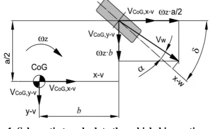
The forces and moments, which constitute right sides of the equations, are functions of vehicle’s kinematic variables. The latter can be derived from the kinematic model, a fragment of which (for the front left wheel) is shown in Fig. 1.

Fig. 1. Schematic to calculate the vehicle kinematic variables

With the longitudinal and lateral CoG velocities and the yaw rate calculated by the system (1), the projections of the wheel linear velocity onto the vehicle coordinate system read:

where is the wheel track and is the distance between the CoG and the wheel axis. In (2) “+” is applied for the left wheels. In (3) “+” is applied for the front wheels. The indices are omitted here and below for brevity.

The sideslip angle is calculated by the following expressions:

where is the steering angle of the wheel, is the steering wheel angle, is the ratio of the steering mechanism.

Having the projections and calculated, one can obtain the magnitude of the wheel velocity vector: . Given this velocity, the sideslip angle, and the wheel angular speed, one can calculate the rolling radius and the longitudinal slip of the wheel [12]:

where is so-called effective rolling radius, which is defined when the wheel is in the free-rolling mode.

Assuming that both the longitudinal slip and the sideslip angles are relatively small (which takes place in low-speed maneuvering at high-adhesion surfaces), the tire forces in the wheel coordinate system and the tire aligning moment ( ) can be calculated as follows: ,

, . In these

formulae, and are the longitudinal and lateral tire-road adhesion coefficients respectively, is the tire pneumatic trail. Calculation of the adhesion coefficients and the pneumatic trail is made by a renowned empirical tire model called the Magic Formula [12]. The tire forces and the aligning moment calculated by this model are translated into the vehicle coordinates using

International Journal of Innovative Technology and Exploring Engineering (IJITEE) ISSN: 2278-3075,Volume-8 Issue-12, October 2019

The following sign convention applies for the third equation of this system: the first term is taken with “+” for the left wheels, the second term is taken with “+” for the front wheels.

III. THE EXPERIMENTAL VEHICLES The experimental vehicle to be converted into an autonomous one was derived from a chassis of a production commercial vehicle, which has undergone substantial modifications [13] (see Fig. 2). The most noticeable of these is removing of the cab – the vehicle is not supposed to be piloted by a human at all. Other modifications included replacement of a conventional powertrain by an electric one consisting of a traction electric drive, a traction battery, and a number of auxiliary systems [14]. Since such deep modifications require a substantial time for implementation, a substitute vehicle (hereafter called the prototyping vehicle) was involved in order to elaborate a prototype of the automated driving system by the time the modified cargo chassis will be available. The vehicle provided by the project’s customer is a passenger car (Fig. 3) equipped with an automatic transmission. Being somewhat far from analogous to a cargo vehicle, the car was nevertheless considered suitable for initial establishment of the automated driving system.

Fig. 2. Modified chassis of a cargo vehicle to be equipped with the automated driving system

Fig. 3. The vehicle used for prototyping of the automated driving system

In order to build the automated driving system, a number of modifications were introduced into the prototyping vehicle. The automation of the longitudinal control is implemented by a drive-by-wire accelerator pedal and an automated hydraulic

braking system. While in the autonomous mode, the signal of the accelerator’s position sensor is replaced by its counterpart sent by the driving automation control system. The automation of the braking system consisted in installation of a solenoid module with electronic controls into the hydraulic braking circuit. Driven by an external command signal, the module regulates the pressure within the circuit. Steering automation was implemented through the torque control of the electric power-steering system.

The tool employed for acquiring and logging of driving trajectories and for providing a positioning feedback into the path-tracking controller is a global navigation satellite system (GNSS) being one of the intensively elaborated means to control autonomous vehicles [4]-[7], [15]. The antennas of this system, installed on the vehicle’s roof, can be seen in Figure 3. The system utilizes the real time kinematic (RTK) methods, which are known for high accuracy of the objects’ positioning and also frequently considered in the literature on autonomous vehicles [5], [6], [16]. The used GNSS also measures the yaw angle and the over-ground velocity by means of the Doppler’s effect.

The second source of information about the vehicle’s motion and its systems’ operation is the onboard CAN bus. In particular, the driving automation control system uses the following signals obtained from this bus: vehicle velocity, wheel rpms, longitudinal and lateral accelerations, yaw rate, steering wheel angle, and angular speeds of the engine and gearbox shafts. In combination with the GNSS data, these signals form a comprehensive state vector of the vehicle dynamics.

Prior to outdoor tests, the vehicle underwent a number of laboratory measurements, including weighing, sizing, determining of the steering ratio characteristics, and some others. The outdoor tests were conducted at a horizontal, asphalt-covered circular track. The testing program included maneuvering with small turning radii at velocities up to 25 km/h.

IV. VALIDATION OF THE MATHEMATICAL

MODEL

In order to validate the model of vehicle dynamics, the tests performed at the track were simulated. In the validating simulations, the trajectory control of the model was driven by the experimental signal of the steering wheel angle logged from the vehicle’s CAN bus. The longitudinal vehicle velocity was controlled indirectly by means of unknown input observers, which calculated the wheel torques based on the rpm signals logged from the CAN. The details on the observer’s design and functioning can be found in [11].

Autonomous Vehicle

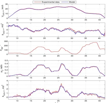
Fig. 4. Comparison between the simulation results and the experimental data for a maneuver performed at the test track by a human driver

In the CAN-acquired experimental data, both longitudinal and lateral accelerations as well as the yaw rate were measured directly by the sensors of the electronic stability control system. The steering angle was measured by a position sensor of the electric power steering system. Comparing the simulation results to the experimental data one can conclude that the model adequacy and accuracy are acceptable. Having similar results obtained for a number of maneuvers, the model of vehicle dynamics was considered appropriate for using in elaboration of the path tracking control system.

V. PATH-TRACKING CONTROL SYSTEM

In the literature on the automated path-tracking control, a number of adaptive control techniques are described and proposed including scheduled gain PID regulators [17], model-based optimal regulators [18], fuzzy logic [19], and sliding mode regulators [20]. Selection of the regulator type for using in this work can be found in [21]. This section describes the regulator only briefly. In estimation of unmeasured external factors like the tire-road adhesion using observers is a prevailing practice; however, the type of regulator employed in this work, being highly adaptive “by the nature”, does not require such observers.

The elaborated path-tracking control system makes use of sliding mode control [22], [23], [24] implemented by a relay regulator described by the following expression:

where is the gain of the relay, and is the sliding surface. In so-called “ideal” sliding mode, the gain has infinite magnitude making the frequency of relay switching infinite as well [22]. However, this obviously cannot be implemented in actual systems; therefore, the gain is set sufficiently large to approach the regulator operation to the “ideal” sliding mode as close as possible.

The sliding surface defines a locus in the regulation error’s state space. The phase trajectory of the system moves along this surface in the “ideal” sliding mode and dwells in some vicinity of this surface in actual sliding modes. The mathematical expression for the sliding surface usually constitutes a linear combination of the tracking error and its derivatives. In the case of the described path-tracking controller, this expression reads as follows:

where is the path-tracking error, and and are parameters defining the orientation of the sliding surface within the state space.

The tracking error is defined in accordance with the schematic shown in Fig. 5. The regulator’s reaction to changes in the curvature of the reference trajectory should be preventive. In order to achieve this, the tracking error is calculated in a certain distance ahead of the vehicle, in a location called the observation point.

International Journal of Innovative Technology and Exploring Engineering (IJITEE) ISSN: 2278-3075,Volume-8 Issue-12, October 2019

being a function of the vehicle velocity and the curvature of the reference path. The reference trajectory is approximated by a piecewise linear function. A segment of this trajectory that is the nearest to the observation point is projected onto the vehicle coordinate system. The intersection of this segment with the lateral axis, which originates from the observation point, gives the tracking error .

Fig. 5. Path-tracking kinematics

Reference trajectories and feedback data for the path-tracking regulator are obtained from the coordinates of the location where the master antenna of the GNSS is mounted. Raw data provided by the GNSS include coordinates in the geocentric system (ECEF), latitude and longitude, and yaw angle. The path-tracking control system operates in two coordinate systems: the stationary system bound to the road surface, and the moving system bound to the vehicle. Translation of raw data into these systems is performed by means of the transfer matrices [4]. The axes of the stationary coordinate system are oriented towards North, East and upwards forming so-called ENU system, which relates to the ECEF system as follows:

where and are the longitude and the latitude of the location. The ECEF coordinates with indices “0” correspond to the origin of the trajectory.

The obtained ENU coordinates of the master antenna together with the yaw angle allow calculating the ENU coordinates of the observation point:

At the next step, the endpoints of the nearest trajectory’s segment are projected from the ENU system onto the moving system, which originates at the observation point:

where and are the ENU

coordinates of the considered endpoint; and are the coordinates of the -th endpoint in the moving system. For the given segment of the trajectory having two endpoints, takes values 1 and 2.

The result of this projecting is a line defined by two points in the moving coordinate system. The path-tracking error , being an intersection of this line with the lateral axis “y-obs” (see Figure 5), is given by:

where is the inclination parameter of the line. As the vehicle moves along the considered linear section of the trajectory, the intersection approaches to one of the endpoints and eventually coincides with it. When this happens, the algorithm switches to the next section. In this manner, the algorithm follows along the reference trajectory. Since the algorithm looks for the nearest section of the trajectory, there is no risk of missing the trajectory due to “jumping” over segments or substantial deviations from the reference path. This feature also allows entering the trajectory from any intermediate point or from a point lying in some (reasonable) distance outside the trajectory.

Autonomous Vehicle

Fig. 6. Comparison between the simulation results and the experimental data for a maneuver performed by a human driver (Experimental data) and the path-tracking controller (Model)

From Fig. 6, one can see an evident resemblance between the human steering control and the automatic control performed by the path-tracking regulator. As a result, the dynamic variables of lateral motion obtained with the automatic control are close to those logged in the field test. In the same manner, a number of other road tests were simulated showing similar outcomes.

VII. CONCLUSIONS AND FUTURE WORK

The article described and showed an implementation of an approach to virtual elaboration and testing of the path-tracking function for autonomous vehicles. The approach consists of two types of simulations, which are based on data obtained from field-testing of the vehicle. The first type implies simulation of the original test performed by a human driver. In order to simulate this, the steering wheel of the model is driven by the angle signal logged in the field test. In the second type of simulation, the steering wheel of the model becomes driven by an automatic path-tracking regulator. The approach allows to compare the automatic control against the human control, find similarities and differences thereof, analyze pros and cons of the automatic control, and devise ways to improve it.

The model of vehicle dynamics described in the article has proven its adequacy and accuracy in comparison against the experimental data obtained by direct measurements. Using this model in combination with the described simulation approach was considered correct in respect of the real-world

operating conditions of the automated driving system. The model of elaborated regulator has shown the control accuracy and quality comparable to that of a human driver.

The sequel of the described work implies implementation of the developed path-tracking system within the prototyping autonomous vehicle. Then the system will be integrated with other driving automation functions and undergo extensive testing and calibration. When both the driving automation system and the modified cargo chassis are completed, the system will be transferred to the chassis and adapted in accordance with the design thereof.

ACKNOWLEDGMENTS

The article was prepared under the agreement #14.624.21.0049 with the Ministry of Education and Science of the Russian Federation (unique project identifier RFMEFI62417X0049).

REFERENCES

1. Industrial Mobility. How autonomous vehicles can change

manufacturing. PricewaterhouseCoopers report, 2018. Avaliable: https://www.pwc.com/us/en/industrial-products/publications/assets/pw c-industrial-mobility-and-manufacturing.pdf

2. J. Guo, P. Hu and R. Wang, “Nonlinear Coordinated Steering and

Braking Control of Vision-Based Autonomous Vehicles in Emergency Obstacle Avoidance”. IEEE Transactions on Intelligent Transportation

Systems, vol. 17(11), 2016, pp. 3230–3240,

International Journal of Innovative Technology and Exploring Engineering (IJITEE) ISSN: 2278-3075,Volume-8 Issue-12, October 2019

3. B. A. Caldato, R. A. Filho and J. E. Castanho, “ORB-ODOM: Stereo

and odometer sensor fusion for simultaneous localization and mapping”. 2017 Latin American Robotics Symposium (LARS) and 2017 Brazilian Symposium on Robotics (SBR). IEEE, November 2017, pp. 5, doi:10.1109/SBR-LARS-R.2017.8215301.

4. A. Angrisano, GNSS/INS Integration Methods. PhD thesis, Parthenope

University of Naples, Naples, 2010, pp. 1-168.

5. B. H. Lee, J. H. Song, J. H. Im, S. H. Im and M. B. Heo, “GPS/DR Error

Estimation for Autonomous Vehicle Localization”. Sensors, vol. 15(8), 2015, pp. 20779-20798; doi:103390/s150820779.

6. A. El-Mowafy, and K. Nobuaki, “Integrity monitoring for positioning of

intelligent transport systems using integrated RTK-GNSS, IMU and vehicle odometer”. IET Intelligent Transport Systems, vol. 12(8), 2018, pp. 901-908, ,doi: 10.1049/iet-its.2018.0106.

7. E. Elisson, Low cost relative GNSS positioning with IMU integration.

PhD thesis, Chalmers University of Technology, Gothenburg, 2014.

8. N. Dicu, G. D. Andreescu and E. Horatiu Gurban, “Automotive

Dead-Reckoning Navigation System Based on Vehicle Speed and Yaw Rate”. 12th International Symposium on Applied Computational Intelligence and Informatic. IEEE, May 2018, pp. 225-228, doi: 10.1109/saci.2018.8440934.

9. P. Yu. Pushkin, and V. V. Erokhin, “Modeling of the trajectory of a dynamic controlled object based on integrated processing of navigation information”. Modern Technologies. System Analysis. Modeling, vol. 4, 2017, pp. 183-188, doi: 10.26731/1813-9108.2017.4(56).

10. M. Zhang, C. Li and K. Liu, “Unmanned Ground Vehicle Positioning

System by GPS/Dead-Reckoning/IMU Sensor Fusion”. Proceedings of the 2nd Annual International Conference on Electronics, Electrical Engineering and Information Science (EEEIS 2016), Advances in Engineering Research, vol. 117, 2017, pp. 737-747, doi: 10.2991/eeeis-16.2017.91.

11. I. Kulikov, and J. Bickel, “Performance analysis of the vehicle electronic

stability control in emergency maneuvers at low-adhesion surfaces”. IOP Conference Series: Materials Science and Engineering, vol. 534, 012009, May 2019, doi:10.1088/1757-899X/534/1/012009.

12. H. B. Pacejka, and I. Besselink, Tire and vehicle dynamics. 3rd ed. Oxford, UK: Butterworth-Heinemann, Elsevier Ltd., 2012, pp: 165-183.

13. A. M. Saykin, S. E. Buznikov, D. V. Endachev, K. E. Karpukhin, and A.

S. Terenchenko, “Development of Russian driverless electric vehicle”. Int. Journal of Mech. Eng. and Tech., vol. 8 (12), 2017, pp. 955-965.

14. A. A. Shorin, K. E. Karpukhin, A. S. Terenchenko, and V. N.

Kondrashov, “Traction module of cab-less unmanned cargo vehicles with electric drive”. Int. Journal of Mech. Eng. and Tech., vol. 9 (11), 2018, pp. 1903–1909.

15. H. Wang, M. Wang, K. Wen and W. Wenqi, “Design and Algorithm

Research of a GNSS/FOG-SINS Integrated Navigation System for Unmanned Vehicles”. Proceedings of the 36th Chinese Control

Conference (CCC), July 2017, pp. 6157-6162, doi:

10.23919/ChiCC.2017.8028336.

16. B. Thuilot, J. Bom, F. Marmoiton and P. Martinet, “Accurate automatic

guidance of an urban electric vehicle relying on a kinematic GPS sensor”. The 5th Symposium on Intelligent Autonomous (issue 13),

IFAC/EURON, July 2004, pp. 53-71, doi:

10.1109/ROBOT.2005.1570755.

17. P. Zhao, J. Chen, Y. Song, X. Tao, T. Xu, and T. Mei, “Design of a

Control System for an Autonomous Vehicle Based on Adaptive-PID”. Int. Journal of Advanced Robotic Systems, vol. 9(2), 2012, pp. 1, doi: 10.5772/51314.

18. M. Alirezaei, S. T. H. Jansen, A. J. C. Schmeitz, and A. K.

Madhusudhanan, “Collision Avoidance System using State Dependent Riccati Equation Technique: An Experimental Robustness Evaluation”. The 13th International Symposium on Advanced Vehicle Control (AVEC'16), September 2016, pp. 127-132.

19. J. Pérez, V. Milanés, and E. Onieva, “Cascade Architecture for Lateral

Control in Autonomous Vehicles”. IEEE Transactions on Intelligent Transportation Systems, vol. 12(1), 2011, pp. 73-82, doi: 10.1109/TITS.2010.2060722.

20. G. Tagne, R. Talj, and A. Charara, “Higher-Order Sliding Mode Control

for Lateral Dynamics of Autonomous Vehicles, with Experimental Validation”, IEEE Intelligent Vehicles Symposium (IV), 2013, doi: 10.1109/IVS.2013.6629545.

21. I. Kulikov, I. Ulchenko, “Performance analysis of the sliding mode control for automated vehicle path tracking at low adhesion surfaces”. Proceedings of 7th International Conference on Traffic and Logistic Engineering, Paris, France, August 2019.

22. V. Utkin, J. Guldner, and J. Shi, Sliding Mode Control in

Electromechanical Systems, 2nd ed. London: CRC Press, Taylor & Francis Group, LLC, 2009.

23. N. Tuan, K. Karpukhin, A. Terenchenko and A. Kolbasov, “World

Trends in the Development of Vehicles with Alternative Energy Sources”. ARPN Journal of engineering and applied sciences, vol. 13(7), 2018, pp. 2535-2542.

24. S. Shadrin, A. Ivanov and K. Karpukhin, “Using Data From Multiplex