Meta Learning for Graph Neural Networks

Rochester Institute of Technology

RIT Scholar Works

Theses

10-2018

Meta Learning for Graph Neural Networks

Rohan N. Dhamdhere

[email protected]

Follow this and additional works at:https://scholarworks.rit.edu/theses

This Thesis is brought to you for free and open access by RIT Scholar Works. It has been accepted for inclusion in Theses by an authorized administrator of RIT Scholar Works. For more information, please [email protected].

Recommended Citation

1 | P a g e

Meta Learning for Graph Neural Networks

By

Rohan N. Dhamdhere

October 2018

A Thesis Submitted in Partial Fulfillment

of the Requirements for the Degree of Master of Science

in

Computer Engineering

Committee Approval:

Dr. Raymond Ptucha, Advisor Date

Assistant Professor

Dr. Andres Kwasinski, Committee Member Date

Professor

Dr. Ifeoma Nwogu, Committee Member Date

Assistant Professor

2 | P a g e

Acknowledgments

This thesis work is the culmination of an important period of my life. I would like to

take this opportunity to thank my advisor Dr. Raymond Ptucha for his continual support and guidance during my master’s degree. I am thankful for Dr. Kwasinski

and Dr. Nwogu for being in my thesis committee. I would like to give a personal

thank you to Miguel Dominguez for getting me involved in the fun research work

that is Graph CNNs. I would also like to thank my family and my close friends,

without their support this journey would not have been as easy as it was. My time

here at RIT was one that I shall remember a long time and would like to thank

3 | P a g e

I dedicate this work to my father, my mother and my sister. For they always supported me

in my quest for excellence.

“Somewhere, something incredible is waiting to be known

.

”

4 | P a g e

Abstract

Deep learning has enabled incredible advances in pattern recognition such as the

fields of computer vision and natural language processing. One of the most

successful areas of deep learning is Convolutional Neural Networks (CNNs).

CNNs have helped improve performance on many difficult video and image

understanding tasks but are restricted to dense gridded structures. Further,

designing their architectures can be challenging, even for image classification

problems. The recently introduced graph CNNs can work on both dense gridded

structures as well as generic graphs. Graph CNNs have been performing at par

with traditional CNNs on tasks such as point cloud classification and segmentation,

protein classification and image classification, while reducing the complexity of the

network.

Graph CNNs provide an extra challenge in designing architectures due to

more complex weight and filter visualization of generic graphs. Designing neural

network architectures, yielding optimal performance, is a laborious and rigorous

process. Hyperparameter tuning is essential for achieving state of the art results

using specific architectures. Using a rich suite of predefined mutations,

evolutionary algorithms have had success in delivering a high-quality population

from a low-quality starter population. This thesis research formulates the graph

CNN architecture design as an evolutionary search problem to generate a

high-quality population of graph CNN model architectures for classification tasks on

5 | P a g e

Contents

Meta Learning for Graph Neural Networks ... 1

Contents ... 5

List of Figures ... 7

List of Tables ... 9

Acronyms ... 10

Chapter 1: Introduction ... 11

1.1Introduction ... 11

1.2 Motivation ... 12

1.3 Contributions ... 13

Chapter 2: Background ... 14

2.1 Deep Learning ... 14

2.2 Convolutional Neural Networks ... 14

2.3 Graph-Convolutional Neural Networks ... 15

A. Spectral Approaches ... 16

B. Spatial Approaches ... 17

2.4 Meta Learning for Architecture search ... 20

Chapter 3: Methodology ... 23

3.1 Graph Convolutional Neural Networks ... 23

A. Graph Convolution ... 24

B. Graph Pooling ... 27

3.2 Architecture Search using Evolutionary Algorithm ... 30

A. Mutations for Evolutionary Algorithm ... 31

B. Fitness Score ... 36

C. Evolutionary Algorithm for Architecture Search ... 36

D. Features of Evolutionary Algorithm ... 38

Chapter 4: Implementation

... 40

4.1 Datasets ... 40

A. Enzymes ... 40

B. MUTAG ... 40

4.2 Implementation ... 41

6 | P a g e

B. Parallel Implementation ... 42

C. Saving and Loading Best model ... 42

Chapter 5: Results and Analysis ... 45

5.1 Results ... 45

A. Comparisons with Other methods ... 45

B. Comparisons with Manual method ... 48

C. Model Architectures ... 48

5.2 Analysis ... 50

A. Mutation Probability Analysis ... 50

B. Weight Loading Analysis ... 51

C. Mutation analysis ... 53

D. Hyperparameter reduction ... 55

Chapter 6: Conclusions and Discussions ... 57

6.1 Conclusions... 57

6.2 Discussions ... 57

6.3 Future works ... 58

Bibliography ... 59

7 | P a g e

List of Figures

Figure 2.2.1: A 2D convolution operation [33]. ... 15

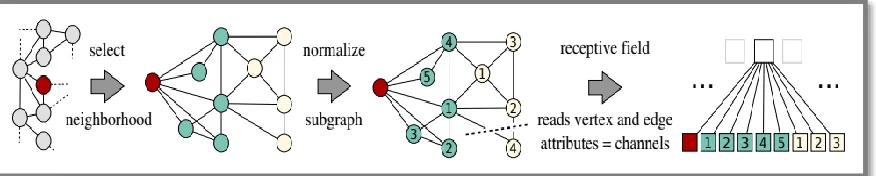
Figure 2.3.1: The PATCHY-SAN algorithm used to find fixed size vector representations of the graph. [18] ... 18

Figure.2.3.2: Graph CNN proposed by FeaStNet [29], where each node in the input patch is associated in a soft manner to each of the M weight matrices based on its features using the weight 𝑞𝑚𝑥𝑖, 𝑥𝑗. [29] ... 19

Figure 2.4.1: The XOR problem and solutions based on genetic search methods. [10] ... 20

Figure 2.4.2: Evolutionary algorithm proposed by Suganuma et al. [1] ... 22

Figure 3.1.1: An example graph and the corresponding vertex matrix and adjacency matrix... 24

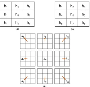
Figure 3.1.2: (a) Learnable parameters in 1-hop graph filters. (b) Classical 3×3 convolution filters. (c) Illustration of eight different edge connections combined to form a 3 × 3 filter. [22] ... 26

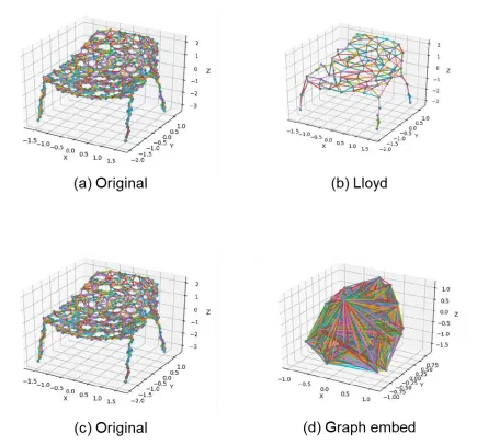
Figure 3.1.3: (a) and (c) show the original 3D mesh graph of chair. (b) shows the 3Dmesh graph after Lloyd pooling. (d) shows the 3D mesh graph after Graph embed pooling. It can be inferred that graph embed pooling is a dense pooling method. [14] ... 30

Figure 3.2.1: Graph convolution layer mutation. ... 31

Figure 3.2.2: Fully-connected layer mutation. ... 31

Figure 3.2.3: One-by-one graph convolution layer mutation. ... 32

Figure 3.2.4: Graph attention layer mutation. ... 33

Figure 3.2.5: Skip connection mutation. ... 33

Figure 3.2.6: Lloyd pooling mutation. ... 33

Figure 3.2.7: Graph embed pooling mutation. ... 34

Figure 3.2.8: Reduced max pooling mutation. ... 34

8 | P a g e

Figure 3.2.10: The flow diagram of Test-and-Mutate-with-Probability algorithm. .... 38

Figure 4.2.1: Loss explosion within training of a fold of an architecture. ... 43

Figure 5.1.1: Model evolution over cycles for (a) Mutag dataset and (b) Enzymes

dataset. ... 47

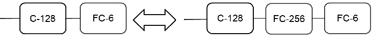
Figure 5.1.2: (a) Best architecture designed manually. (b) Best architecture

generated by evolution. ... 49

Figure 5.1.3: (a)Best architecture designed manually. (b) Top architectures

generated by evolution. ... 50

Figure 5.2.1: Top row (Fig. (a), (b)) are experiments with no probability associated

with mutations (baseline algorithm). Bottom row (Fig. (c), (d)) are experiments with

probabilities associated with mutations. ... 51

Figure 5.2.2: This figure emphasizes the importance of weight loading. Fig. (a) is

based on experiment which involved no weight loading, Fig (b) is based on

experiment with weight loading. ... 53

Figure 5.2.3: Evolution of different mutations’ probability over cycles. (a) shows the

‘add’ mutations and their probability change over cycles. (b) shows the ‘remove’

mutations and their probability change over cycles. (c) shows the pooling and

parameter mutations and their change over cycles. All these figures show the

9 | P a g e

List of Tables

Table 4.1: Summary of protein datasets to be used in this thesis. ... 41

Table 5.1.1: 10-fold cross validation accuracy score comparisons between different

methods. ... 46

Table 5.1.2: Comparison of running times and best accuracy scores between

10 | P a g e

Acronyms

CNNs

Convolutional Neural networks

Graph-CNNs

Graph Convolutional Neural Networks

MLP

11 | P a g e

Chapter 1

Introduction

1.1 Introduction

Neural networks can successfully execute challenging tasks when provided with

abundant data along with sizable computational resources. Convolutional Neural

Networks (CNNs) have broken traditional computer vision barriers and achieved high

quality results on image classification and segmentation tasks [7, 8, 19]. CNNs are

helping deep learning get embedded into newer fields every day. CNNs have the

ability to simultaneously automate the process of feature extraction and classification.

This ability of CNNs is helping them beat other machine learning algorithms at several

tasks.

CNNs are highly successful in tasks involving data represented in discrete

gridded structures such as image, videos etc. Unstructured data (e.g.: 3D Point clouds

or 3D meshes [26, 27]) or data that cannot be represented in such gridded structures

(e.g.: Protein graphs [21, 24, 25]) cannot be filtered by conventional convolution

operations, and therefore CNNs have enjoyed very little success in tasks involving

such data. Most unstructured data can easily be processed into graphs. This has led

to the development of different convolutional operators for graph data and has led to

the research field of Graph CNNs [12, 14, 18, 22].

Graph CNNs have shown comparable to state-of-the-art performances on

classification tasks of protein graphs, 3D point clouds and images [12, 14]. They have

also performed well on image and 3D segmentation tasks [29] as well as classification

of functional MRIs of brain [28]. With graph CNNs, Convolutional Neural Networks can

12 | P a g e Although CNNs can automatically extract and perform classification of

features, they need precise hyperparameters and optimal architectures to achieve

high accuracy and precision. Solving for hyperparameters and designing architectures

are typically done by a human expert. This is a laborious process and requires high

amount of focus and experience. Designing CNN architectures is a tough task even

for image data where visualization of weights and filters aid the process of design.

Graph CNNs work on unstructured data which are converted to graphs. Visualizations

of weights and filters of graph CNNs inform abstract knowledge about the data. Due

to the difficulty of weight visualization, the process of designing graph CNNs is extra

challenging compared to conventional CNNs.

Research to automate the process of neural network design has been going

on for few decades with early work being related to automating Multi-Layer Perceptron

(MLP) based neural network design [2, 3, 10, 13]. In recent years, many approaches

like reinforcement learning [30, 31], genetic algorithms [6] and evolutionary algorithms

[1,17] have been used to automate the process CNN architecture design and

hyperparameter search. This process has had some success on standard image

datasets like CIFAR [32]. This work attempts automate the process of graph CNN

architecture design and hyperparameter search using evolutionary algorithms for the

classification of protein graph structures.

1.2 Motivation

Designing of any neural network is laborious process. After designing, tuning of

hyperparameters is another time-consuming task. This work is an extension of

previous work which was done for classification of protein graphs by designing custom

graph CNNs manually. The difficulty of the previous research motivated the

automation of various parameters required for graph CNN design. Also, this work is a

feasibility check on whether evolutionary algorithms are able to generalize over

different datasets and find top performing architectures tailored for specific datasets.

Many other works on automation of CNN architecture design use abundant

computing resources. This work attempts to find out if evolutionary search for

13 | P a g e and what are the modifications required to make the algorithm more computationally

efficient. Discovering tangible answers to the above mentioned problems related

architecture design is the main motivation for this work.

1.3 Contributions

The main contributions of this thesis work can be summarized as:

• An evolutionary algorithm for graph CNNs based on probabilistic mutation

strategy.

• Achieve better than human performance on benchmark protein datasets using

same graph CNN method.

• Parallel implementation of cross validation evaluation for evolution of models.

• Selective loading of weights based on layers present in previous architectures.

• Saving and loading of best trained models using training loss for boosting

14 | P a g e

Chapter 2

Background

2.1 Deep Learning

Deep Learning has provided breakthrough research results in many fields. Deep

learning network’s ability to extract its own features for classification has provided it

an edge over other machine learning techniques. It has especially helped computer

vision research by providing better feature descriptors than traditional computer vision features like HoG, SIFT etc. [46, 47]. Also, it has reduced the feature designer’s bias

introduced in the extracted features. All these merits have resulted in deep neural

networks being the method of choice for feature extraction along with MLP classifiers.

2.2 Convolutional Neural Networks

Much of the success achieved by deep learning can be attributed to CNNs. CNN

architectures have performed exceptionally well on tasks related to image or video

data classification and understanding [7, 8, 19]. CNNs extend the capabilities of MLPs

while keeping a similar number of parameters. CNNs make use of localized

information by using a common filter over the full input. Parameter sharing over

different regions of the input results in sharing of localized features. A CNN layer can

be defined as in (2.2.1), where

𝑉

network, for pixel i, j at the cth _{channel, where channel is the third dimension of the}

image volume. Here, at any layer, image volume V is convolved with a convolutional

filter volume W to get convolved image volume V.

15 | P a g e

Figure 2.2.1: A 2D convolution operation [33].

Much power of CNNs is derived from the common set of parameters shared

over different inputs. Their limitation is that the input needs to be gridded with fixed

neighbors. Graph Convolutional Neural Networks (Graph CNNs) remove this limitation

using Graph-based Convolution operation.

2.3 Graph-Convolutional Neural Networks

Research to broaden the extent of neural networks to graph structured data has had

substantial success in recent times. A graph G is represented using a tuple (V, A) -

vertices V and adjacency matrix A. The adjacency matrix entries can be defined as in

(2.3.1).

𝑎

= {

𝑤

, 𝑖𝑓 𝑡ℎ𝑒𝑟𝑒 𝑖𝑠 𝑎𝑛 𝑒𝑑𝑔𝑒 𝑏𝑒𝑡𝑤𝑒𝑒𝑛 𝑖 𝑎𝑛𝑑 𝑗

0, 𝑜𝑡ℎ𝑒𝑟𝑤𝑖𝑠𝑒

(2.3.1)

The scalar 𝑤_𝑖𝑗 is a weight that represents some measure of strength of the

edge between vertex i and vertex j. The research of graph convolutional networks

follows two broad general approaches to generalizing CNNs to graph data: spectral

16 | P a g e

A.

Spectral Approaches

Spectral approaches use spectral graph theory. Spectral graph theory works in the

spectral domain by constructing a filter based on the eigenvector decomposition of the

Graph Laplacian L shown in (2.3.2).

𝐿 = 𝐷 − 𝐴

(2.3.2)

𝐿 = 𝐼 − 𝐷

𝐴𝐷

(2.3.3)

L can be normalized as shown in (2.3.3), where A is the adjacency matrix of

the graph, D is the diagonal degree matrix and I is the identity matrix. L can be used

to compute an eigenbasis U. This eigenbasis U is similar to the Discrete Fourier

Transform (DFT). A graph signal x can be transformed into spectral domain and

multiplying each frequency by a filter h, to get its filtered output in spectral domain.

This is illustrated in (2.3.4), where ⊙ is the elementwise product and ‘.’ represents the

matrix multiplication.

𝑥 ∗ ℎ = 𝑈

. (𝑈𝑥 ⊙ ℎ)

(2.3.4)

Thus, the filtering operation in the spectral domain is performed multiplying filter

coefficients with spectrally transformed graph signals. Many works propose graph

CNN models based on this method of filtering [34, 35, 37]. One of the major practical

limitations of spectral domain-based learning of filters is the necessity of input graph

samples to be homogenous for converting graphs to Laplacian matrix. This is

necessary as the eigenbasis of the Graph Laplacian needs to be solved separately for

every unique graph structure. Most spectral works tend to focus on experiments

where there is a single graph structure common across all samples, like a single large

social network graph. Spatial approaches are advantaged over spectral methods in

17 | P a g e

B.

Spatial Approaches

To achieve better generalization across graphs, various works follow a local

neighborhood graph filtering strategy. They generally require advanced data

preprocessing techniques for learning to process neighborhoods that are different

sizes and structures for each vertex. These methods differ in how they find a

correspondence between filter weights and nodes in local graph neighborhoods.

Bruna et al. [38] assumed fixed graph structure and does not share weights

among neighborhoods. Duvenaud et al. [39] sums the signal over neighboring vertices

followed by a weight matrix multiplication, effectively sharing the same weights among

all edges. Diffusion Convolutional Neural Networks (DCNNs) [40] arrange vertex

features based on sequence of hops from different starting vertices to encode a graph

into matrix layers.

Similar to Petroski Such et al. [5], DCNNs use polynomials of the adjacency

matrix to define convolutional filters. They also use global vertex mean pooling to

obtain a vector representation of the graph. The diffusion process of DCNNs is shown

in (2.3.5), where Zt is the output feature vector for the vertices on the graph Gt , f is

the activation function, Wc is a learnable weight-matrix, 𝑃_𝑡∗ is a degree-normalized

polynomial of the adjacency matrix At , and Xt is the input feature vector for the vertices

on the graph Gt. (⊙ is the elementwise product)

𝑍

= 𝑓(𝑊

⊙ 𝑃

𝑋

)

(2.3.5)

Niepert et al. [18] rely on a heuristic ordering of the nodes, and then apply 1D

CNNs. They linearize the graphs using a method called PATCHY-SAN. Using graph

search algorithms, PATCHY-SAN attempts to obtain fixed size feature vector

18 | P a g e

Figure 2.3.1: The PATCHY-SAN algorithm used to find fixed size vector representations of the

graph. [18]

Simonovsky et al. [12] generate conditioned filter weights for edge labels.

These weights are generated dynamically for every input to the graph. This edge

conditioned convolution operation is given in (2.3.6), where 𝑋𝑙_{(𝑖) is the current layer}

signal to be computed, N(i) is the neighborhood of vertex i, 𝜃_𝑗𝑖𝑙 is the edge-weight

matrix, 𝑋𝑙−1_{(𝑗) is the previous layer signal and 𝑏}𝑙 _{is the learnable bias. The}

edge-weights 𝜃_𝑗𝑖𝑙 are given as per (2.3.7), where L(j, i) is the given class label. 𝐹𝑙 _is

parameterized with learnable network weights 𝑤𝑙_{. The model parameters 𝑤}𝑙 _and𝑏𝑙

update during training and dynamically generate 𝜃_𝑗𝑖𝑙 for an edge label in input graph.

𝑋

(𝑖) =

|𝑁(𝑖)|

∑

𝜃

𝑙

𝑋

(𝑗)

𝑗∈𝑁(𝑖)

+ 𝑏

(2.3.6)

𝜃

= 𝐹

(𝐿(𝑗, 𝑖); 𝑤

)

(2.3.7)

The main challenge in the case of irregular data graphs is to define the

correspondence between neighbors and weight matrices. FeaStNet [29] proposes to

establish this correspondence in a data-driven manner, using a function over features

computed in the preceding layer of the network, and learning the parameters of this

function as a part of the network. They propose a similar approach to [12]. Instead of

assigning each neighbor j of a node i to a single weight matrix, we use a

soft-assignment 𝑞𝑚(𝑥𝑖, 𝑥𝑗) of the j-th neighbor across all the 𝑀 weight matrices. The

activation 𝑦_𝑖 ∈ ℝ𝐸 _{of pixel i in the output feature map using the soft assignments is}

defined as in (2.3.8), where b ∈ ℝ𝐸 _{is the vector of bias terms, 𝑞}

19 | P a g e assignment of 𝑥_𝑖 to the m-th weight matrix, and 𝒩_𝑖 is the set of neighbors of i (including

i), and |𝒩𝑖| its cardinal.

𝑦

= 𝑏 + ∑

|𝒩_𝑖|

∑

𝑞

(𝑥

, 𝑥

)𝑊

𝑥

𝑀

𝑚=1

(2.3.8)

They use Mahalanolbis distance based soft assignment in feature space to determine

local filters dynamically based on previous layers of the network. Their approach is

illustrated in Figure 2.3.2.

Figure.2.3.2: Graph CNN proposed by FeaStNet [29], where each node in the input patch is

associated in a soft manner to each of the M weight matrices based on its features using the weight 𝑞𝑚(𝑥𝑖, 𝑥𝑗). [29]

Similar to earlier mentioned spatial methods, Such et. al. [22] use local edge features

for graph convolution, done by convolving on adjacency matrix of the graph. They

introduce vertex graph filters helping to learn on both graph vertex and edges

simultaneously. Pooling in traditional CNNs helps to increase the receptive field of the

filter and thereby helps to learn higher order features. They introduce pooling for

graphs which is further explored by Dominguez et. al [14] to provide deep graph

networks for 3D point cloud classification.

In this thesis work, graph convolution and pooling operations introduced in

Such et. al. [22] and Dominguez et. al. [14] are used as the base operations for building

20 | P a g e

2.4 Meta Learning for Architecture search

CNNs architectures have been able to achieve state-of-the-art performance on a

variety of tasks. There are many popular architectures, each of which can be used on

a broad variety of data. For example, AlexNet, VggNet, ResNet, DenseNet [7, 9, 41,

42] are popular CNN architectures available for users to develop a neural network

based prediction model for the user defined task. Each of these architectures were

manually designed by expert humans. These designers leverage their in-depth

knowledge about CNN training and optimization to define these architectures.

These popular architectures are flexible and generalize well to a variety of data

but often need optimized hyperparameter tuning or custom architecture modifications

for good performance. This process of designing neural network architectures is

arduous and requires focused human attention. Also, hyperparameter tuning is time

consuming and tedious.

Research to automate the design of neural networks has a long but sporadic

history. Miller et al. [10] used genetic-search based methods to evolve MLP based

neural networks to automate the task of network design. Initially, the evolution was

only restricted to only evolving weights of static architectures. They were successful

to solve the XOR problem, a big test at the time and Figure 2.3.1 shows some of the

evolved architectures for the same.

21 | P a g e “Evolving Neural Networks through Augmenting Topologies” [13] did

simultaneous adaption of weights and architectures. They defined basic mutations for evolution:

i. Modify a weight.

ii. Add a connection between existing nodes.

iii. Insert node while splitting existing connection.

These evolutionary algorithms are not sufficient for deep neural networks.

Current research directions focus on reinforcement learning and evolutionary

strategies for the solving the neural architecture search problem. Both these directions

have focused on allowing building of CNN architectures resembling those designed

manually by humans.

Reinforcement learning based approaches have been able to achieve more

success on real-world image data related classification tasks. Most reinforcement

learning based approaches use indirect encoding schemes for network

representation. Zoph et al. [31] used reinforcement learning on a deeper fixed-length

architecture, adding one layer at a time. Their mutations included addition/removal of

skip connections as well as tunable hyperparameters. Baker et al. [30] used

Q-learning to discover networks. They made architectures more flexible by allowing the

algorithms to decide the number of layers in the network. This allows the network to

adapt to the dataset at hand and construct shallow or deep solutions as necessary.

Progressing from earlier works, evolutionary approaches later combined with

back-propagation [1, 17, 43] to evolve architectures and tune hyperparameters

simultaneously. These approaches introduce architectural mutations and weight

back-propagation. More recent approaches [43] added weight inheritance for architectures.

Suganuma et al. [1] use a direct encoding type approach using Cartesian Genetic

Programming (CGP) [44] for their evolutionary process as shown in Figure 2.3.2. They

define functional blocks such as ConvBlock, ResBlock etc. as functional blocks or

22 | P a g e

Figure 2.4.2: Evolutionary algorithm proposed by Suganuma et al. [1]

This work is uses evolutionary approaches similar to Real et al. [17] and Graph

CNN defined by Dominguez et. al. [14] as the base model and built an evolutionary

23 | P a g e

Chapter 3

Methodology

3.1 Graph Convolutional Neural Networks

A Graph can be decomposed into two main elements, the graph vertices vij and

graph edges aij. A graph signal can be represented as a tuple described in (3.1.1)

𝑮 = ( 𝑽, 𝑨)

(3.1.1)

where 𝑽 𝜖 ℝ𝑁 × 𝑓 _{is the vertex signal matrix describing 𝑁 vertices with 𝑓 features}

each. 𝑨 𝜖 ℝ𝑁 × 𝑁 represents the adjacency matrix which encodes the edge

information with its elements as defined Chapter 2. Each entry in 𝑨 is defined as per

(3.1.2) previously defined in (2.3.1),

𝑎

= {

𝑤

, 𝑖𝑓 𝑡ℎ𝑒𝑟𝑒 𝑖𝑠 𝑎𝑛 𝑒𝑑𝑔𝑒 𝑏𝑒𝑡𝑤𝑒𝑒𝑛 𝑖 𝑎𝑛𝑑 𝑗

0, 𝑜𝑡ℎ𝑒𝑟𝑤𝑖𝑠𝑒

(3.1.2)

An Illustration of the graph and its corresponding vertex matrix V and adjacency matrix

24 | P a g e

Figure 3.1.1: An example graph and the corresponding vertex matrix and adjacency matrix.

A.

Graph Convolution

Graph data can succinctly represent information in both vertices and edges. To

process and learn the information, the convolution filtering technique for graphs must

account for filtering both vertex information and edge information. This work uses the

Graph convolution model proposed by Such et al. [22]. This is a spatial approach

related graph convolution method following the local neighborhood graph filtering

strategy. The graph convolution operation is based on the polynomials of the graph

adjacency matrix and is similar to the convolution defined by Sandryhaila et al. [36] as

25 | P a g e

𝐻 = ℎ

𝐼 + ℎ

𝐴

+ ℎ

𝐴

+ ℎ

𝐴

+ ⋯ + ℎ

𝐴

(3.1.3)

The filter is defined as the kth_{-degree polynomial of the graph’s adjacency}

matrix. The exponent of polynomial encodes the number of hops from a given vertex

that are being multiplied by the given filter tap. The scalar coefficients ℎ_𝑖 control the

contribution of the neighbors of a vertex during the convolution operation. The filter

matrix thus obtained is 𝐻 ∈ ℝ𝑁 × 𝑁_{. To convolve the vertices 𝑉 with the filter 𝐻 is a}

matrix multiplication shown in (3.1.4), where 𝑉_𝑜𝑢𝑡, 𝑉_𝑖𝑛 ∈ ℝ𝑁.

𝑉

= 𝐻𝑉

(3.1.4)

Such et al. [22] adjust this model in three ways. First, they avoid the

exponentiated A and simplify the polynomial of adjacency in (3.1.3) to be linear as

shown in (3.1.5). This is done because a cascade of filters can effectively approximate

the receptive field of a single large filter as shown by VGGNet [41].

𝐻 ≈ ℎ

𝐼 + ℎ

𝐴

(3.1.5)

Second, they construct an adjacency tensor 𝓐. This tensor contains multiple

adjacency matrices 𝓐_𝓵 as the slices of adjacency tensor. Each slice encodes a

particular edge feature and thus the linear filter matrix from (3.1.5) is defined as a

convex combination of each adjacency matrix as in (3.1.6) and concisely as in (3.1.7).

𝐻 = ℎ

𝐼 + ℎ

𝐴

+ ℎ

𝐴

+ ⋯ + ℎ

𝐴

(3.1.6)

𝐻 ≈ ∑

ℎ

𝐴

(3.1.7)

Multiple adjacency matrices encode multiple edge features, each encoding a

single feature. Also, partitioning the edges into multiple matrices conveys a sense of

26 | P a g e default Graph CNN linear filter in an image application. A given filter tap is applied to

all vertices of a given distance, isotropically (no sense of ‘direction’). In this case, ℎ0

is applied to the 0-hop vertex and ℎ₁ is applied to all adjacent vertices. If another

border of pixels surrounded this figure, each pixel in that border would be multiplied

by a filter tap ℎ₂.

The Figure 3.1.2(c) shows that the adjacency matrix can be partitioned into

nine adjacency matrices to form an adjacency tensor. Each partitioned adjacency

matrix represents a different relative connection (edge feature) to a given vertex. Now

a unique filter is applied to every adjacency matrix and aggregated to perform

convolution. This induces a sense of direction into the Graph CNN filter making it

anisotropic. This is equivalent to a 3 x 3 FIR filter in conventional CNN applications

(Figure 3.1.2(b)).

Figure 3.1.2: (a) Learnable parameters in 1-hop graph filters. (b) Classical 3×3 convolution filters.

27 | P a g e All these filters are described for a single vertex feature. To extend to multiple

vertex features, each ℎℓ needs to be in ℝ𝐶 making H of dimension ℝ𝑁×𝑁×𝐶. Thus,

every vertex feature has a N * N filter matrix H. So (3.1.7) can be modified as in (3.1.8)

where 𝐻(𝑐) _{is an N * N slice of H and 𝒉}(𝒄) _{` is a scalar corresponding to a given input}

feature and a given slice of 𝐴ℓ.

𝐻

≈ ∑

ℎ

𝐴

(3.1.8)

The vertex signal is filtered using the 𝐻(𝑐) as described in (3.1.9) where

𝑉_𝑖𝑛(𝑐) is the column of 𝑉_𝑖𝑛 that only contains vertex feature c. We also add a bias b ∈ ℝ.

This results in 𝑉_𝑖𝑛 ∈ ℝ𝑁.

𝑉

= ∑

𝐻

𝑉

+ 𝑏

(3.1.9)

This is how graph convolution is defined on a graph with multiple vertex features and

edge features by Such et al. [22]. This approach is used for this thesis work.

B.

Graph Pooling

The pooling operation can be dissected in two parts: the coarsening of structure and

the reduction of signal on that structure. In grid structures such as images, the

coarsening of structure is implicitly understood. But for graphs, such as protein

structures, every sample can have a unique structure. Dominguez et al. [14] defined

various pooling frameworks for graphs. These will be described here in succession.

The first method they proposed is Lloyd Algebraic graph pooling on graphs that can

28 | P a g e a. Lloyd Algebraic graph pooling:

In this, a coarsening operator P is defined to reduce the Graph G = (V,A) with

N1 vertices to Greduced = (Vreduced,Areduced) with N2 vertices. P is a N1 × N2 matrix

with its elements defined as in (3.1.10).

𝑷

= {

𝐶, 𝑖𝑓 𝑖

𝑣𝑒𝑟𝑡𝑒𝑥 𝑜𝑓 𝑮 𝑖𝑠 𝑢𝑠𝑒𝑑 𝑡𝑜

𝑑𝑒𝑓𝑖𝑛𝑒 𝑡ℎ𝑒 𝑗

𝑜𝑓 𝑮

.

0, 𝑜𝑡ℎ𝑒𝑟𝑤𝑖𝑠𝑒

(3.1.10)

C is determined by mapping the graph clustering method used in mapping

“fine” vertices to the “coarsen” vertices. Distances are calculated by finding the

shortest path on a graph using the Bellman Ford algorithm. Using the

coarsening operator P, Areduced_{is defined using (3.1.11) and V}reduced _{is defined}

using (3.1.12) through (3.1.14). Sum, average, and max pooling are defined

using (3.1.12), (3.1.13), and (3.1.14) respectively.

𝐴

= 𝑃

𝐴𝑃

(3.1.11)

𝑉

= 𝑃

(𝑉)

(3.1.12)

𝑉

= 𝑃ˆ

(𝑉)

(3.1.13)

𝑉

= 𝜙

(𝑉)

(3.1.14)

Element 𝑨_𝒊,𝒋𝒓𝒆𝒅𝒖𝒄𝒆𝒅 can be thought of as the aggregation of all the weights of

edges while coarsening the graph G to Greduced_{. 𝑷ˆ}𝑻 _{is the column-sum normalized}

version of P. Also, 𝜙_𝑃 is a non-linear max pooling function. Here in this work we

used only max pooling. Thus, the graph structure is reduced by (3.1.11) and the

29 | P a g e b. Graph Embed Pooling:

Such et al. [5, 22] introduced graph embed pooling for graphs. It is a dense

pooling method but fits the structure of Algebraic pooling. Graph embed pooling

learns a fully connected layer whose output is treated as an embedding matrix that

produces a fixed size output. To produce a pooled graph reduced to a fixed N’

vertices, the learned filter taps from this pooling layer produce an embedding

matrix 𝑉_𝑒𝑚𝑏 ∈ ℝ𝑁×𝑁′. Like in (3.1.9), a filter tensor 𝐻_𝑒𝑚𝑏 ∈ ℝ𝑁×𝑁×𝐶×𝑁′ _{is learned}

and multiplied by the vertices to produce a filtered output as shown in (3.1.15).

𝑉

= ∑

𝐻

𝑉

+ 𝑏

(3.1.15)

𝑉_𝑒𝑚𝑏(𝑛′) is column wise stacked up to form the matrix 𝑉_𝑒𝑚𝑏. Softmax function is used

for normalization of values of 𝑉_𝑒𝑚𝑏 as in (3.1.16). Equations (3.1.17) and (3.1.18)

show how 𝑉_𝑒𝑚𝑏 pools the graph data.

𝑉

= 𝜎(𝑉

)

(3.1.16)

𝑉

= 𝑉

𝑉

(3.1.17)

𝐴

= 𝑉

𝐴

𝑉

(3.1.18)

The above equations represent the graph embed pooling defined by Such et al.

[22] and Dominguez et al. [14]. Figure 3.1.3 illustrates both the graph pooling

30 | P a g e

Figure 3.1.3: (a) and (c) show the original 3D mesh graph of chair. (b) shows the 3Dmesh graph

after Lloyd pooling. (d) shows the 3D mesh graph after Graph embed pooling. It can be inferred that graph embed pooling is a dense pooling method. [14]

3.2 Architecture Search using Evolutionary Algorithm

This work uses evolutionary algorithms for searching architectures in graph

convolution neural networks. A set of mutations are defined which the architectures

can choose to improve their fitness scores and maximize the fitness function. Added

features of the evolutionary algorithm help in speeding up the architecture search

while achieving good fitness scores. This section explains in detail the evolutionary

31 | P a g e

A.

Mutations for Evolutionary Algorithm

For architecture search using evolutionary methods, it is important to define mutations

that can find improved architectures or hyperparameters that would raise the fitness

score of the architecture. There are 3 types of mutations:

a. Architectural change mutations:

These mutations change the architecture of the network by adding or removing

layers from the previous architecture. These mutations are as follows:

i. Adding / Removing a graph convolution layer:

In this mutation a graph convolution layer is added to or removed from a

randomly chosen position in the current network architecture. While adding, the

number of output filters of the new convolution layer are randomly chosen from

[128, 256, 512]. An example mutation is shown in Figure 3.2.1.

Figure 3.2.1: Graph convolution layer mutation.

ii. Adding / Removing a fully-connected layer:

In this mutation a fully-connected layer is added to or removed from a randomly

chosen position in the current network architecture. While adding, the number of

units of the new fully-connected layer is a randomly chosen value x, where x ∈

(output_classes,500]. This mutation is shown in Figure 3.2.2.

32 | P a g e

iii. Adding / Removing a one-by-one graph convolution layer:

One-by-one convolution were proposed by Lin et al. [48]. These are used to

alter the size of the channel dimension c of the convolution filters. They also

require less parameters to change the channel size when compared to the 33 filter. One-by-one graph convolution is same as the one-by-one normal

convolution. In this mutation a one-by-one graph convolution layer is added to

or removed from a randomly chosen position in the current network

architecture. One-by-one convolution helps in reducing dimensionality in filter

dimension. While adding, the number of output filters of the new one-by-one

layer are randomly chosen from [128, 256, 512]. This mutation is shown in

Figure 3.2.3.

Figure 3.2.3: One-by-one graph convolution layer mutation.

iv. Adding / Removing a graph attention layer:

In this mutation, a graph attention layer is added to or removed from a randomly

chosen position in the current network architecture. This attention layer is a soft

attention. It learns attention over the vertices by weighing the vertex features. The

attention is given by (3.2.1) and applied on the vertices as given in (3.2.2), where

𝑉is the vertex graph signal, 𝑤 is the vertex feature, 𝛼 is the attention vector and

𝑉 ∈ ℝ𝐵×𝑁×𝐹_{, 𝑤 ∈ ℝ}𝐹_{, 𝛼 ∈ ℝ}𝑁

𝛼 = softmax(𝑉𝑤)

(3.2.1)

𝑉

= 𝛼

𝑉

(3.2.2)

While adding, the number of output filters of the new attention layer are

33 | P a g e

Figure 3.2.4: Graph attention layer mutation.

v. Adding / Removing a skip connection:

In this mutation, a skip connection path is added or removed between randomly

chosen graph convolution layers in the current network architecture. This mutation

is shown in Figure 3.2.5.

Figure 3.2.5: Skip connection mutation.

b. Graph structure change mutation:

These mutations are responsible for changing the graph structure to increase the

receptive field of the filters applied on them. These help in understanding high

level features in the graphs. These mutations are as follows:

i. Pooling mutation:

In this mutation, the graph structure is changed using max pooling defined in

(3.1.11) and (3.1.12). The pooling ratio is a randomly chosen value x where x ∈

(0,1]. The pooling layer is added at a randomly chosen position in the current

network. This mutation is shown in Figure 3.2.6.

34 | P a g e

ii. Graph embed pooling mutation:

In this mutation, the graph structure is changed using graph embed pooling

defined in (3.1.15) and (3.1.16). The pooled number of vertices is randomly chosen

from [16,32,64]. The pooling layer is added at a randomly chosen position in the

current network. This mutation is shown in Figure 3.2.7.

Figure 3.2.7: Graph embed pooling mutation.

iii. Reduced max layer:

Reduce max operation for a matrix/tensor reduces the matrix/tensor to a single

dimension vector, where each element of the vector is maximum value along

other dimensions of the matrix/tensor. The reduce max mutation changes the

graph structure to a linear feature vector. The reduce max layer is added at the

position before the first fully-connected layer in the current network. There can

be at max. one reduced-max layer in the network. This mutation is shown in

Figure 3.2.8.

Figure 3.2.8: Reduced max pooling mutation.

c. Hyperparameter mutations:

These mutations change some of the different hyperparameters needed to tune

the architecture. These mutations are as follows:

i. Learning rate mutations:

These mutations change the learning rate parameter in different ways. There

are three types of learning rate mutations. When the learning rate mutation is

chosen, a random number of these mutations are chosen and applied to the

35 | P a g e

• Changing starter learning rate:

Starter learning rate is the parameter which decides the learning rate of the

model at the beginning of a model training cycle. In this mutation, the starter

learning rate is changed from an old value to a value randomly chosen from

[0.5×old value, 2×old value]

• Changing learning rate step:

Learning rate step is the parameter which decides the iteration steps of the

model training cycle at which learning rate value is decreased. A model

starts its training cycles with the starter learning rate and after every

learning rate step cycles, the learning rate value is decreased. In this

mutation, the learning rate step is changed from the old value old value to

a value randomly chosen from [0.5×old value, 2×old value]

• Changing learning rate exponential:

Learning rate exponential decides the factor by which the learning rate

value is decreased at the learning rate step in a model training cycle. In this

mutation, the learning rate exponential is changed from the old value to a

value randomly chosen from [0.5×old value, 2×old value]

ii. Regularization mutations:

These mutations change the learning rate parameter in different ways. There

are two types of regularization mutations. When the regularization mutation is

chosen, a random number of these mutations are chosen and applied to the

current architecture. They are:

• L1 regularization: In this mutation, the L1 regularization is changed from the old value old value to a value randomly chosen from [0.5×old value, 2×old

value]

• L2 regularization: In this mutation, the L2 regularization is changed from the old value old value to a value randomly chosen from [0.5×old value, 2×old

36 | P a g e

B.

Fitness Score

For evaluating the success of a mutation, it is important to define a good metric as the

fitness score. In the case of architecture search of graph CNNs for classification tasks,

the accuracy of the network is a good measure to evaluate the performance of the

architecture. But this accuracy score must be on unforeseen data. Hence, in this case,

this work uses validation accuracy score as fitness score metric for architecture

search.

C.

Evolutionary Algorithm for Architecture Search

Architecture design is a laborious and resource intensive process. Evolutionary

algorithms used for its automatic discovery must increase its efficiency of resource

usage and improve the time taken for reaching optimal performance compared to

manual architecture design. For this task, this research defines a baseline evolutionary

algorithm model and then introduces an improved evolutionary algorithm model which

reduces the training time and converges to better solutions faster.

a. Test-and-Mutate Algorithm (Baseline):

In this algorithm, all the N models in the pool are trained for the first cycle and for every

next cycle two random models are chosen and compared based on their validation

accuracy scores. The best model from the chosen two are mutated. Mutation is

selected randomly from all the available mutations. Mutated model is trained, and its

validation accuracy is compared with the two chosen models. If it is better than either

of the two chosen models, the worst model is replaced with the mutated model in the

37 | P a g e

Figure 3.2.9: The flow diagram of Test-and-Mutate algorithm.

b. Test-and-Mutate-with-Probability Algorithm:

This algorithm is an improvement over the baseline Test-and-Mutate baseline

algorithm described above. The model training and selection process remains same

as in the baseline algorithm. The mutation process is improved. In the First cycle, all

mutations are assigned equal selection probabilities. Based on the helpfulness of the

mutation a constant reward is added or subtracted from the mutation’s selection

probability. The changed mutation selection probabilities are applied to the mutation

selection process after every p cycles. The flow of this algorithm is shown in the Figure

38 | P a g e

Figure 3.2.10: The flow diagram of Test-and-Mutate-with-Probability algorithm.

D.

Features of Evolutionary Algorithm

The improved evolutionary algorithm Test-and-Mutate-with-Probability has some

salient features that helps the algorithm converge to better graph CNNs architectures.

These salient features are as follows:

a. Mutation probability:

In this algorithm, every mutation is assigned a selection probability. All the

mutations are assigned equal selection probabilities at the training cycle. This

selection probability changes every cycle a model is replaced with a better model

architecture.

b. Mutation probability reward:

Every mutation selection probability is changed by a factor of the mutation

probability reward. The Mutation probability reward is set value between (0,1). If

39 | P a g e is multiplied by a factor of (1.0 + reward). If the mutation is unsuccessful in replacing an architecture, the mutation probability is multiplied by a factor of (1.0 –

reward).

c. Mutation probability cycle:

The mutation selection probability value is changed and stored after every cycle

based on the replacement of the model architecture. The mutation probability cycle

decides the update cycle, when the most current mutation selection probabilities

are used for the process of model selection. The mutation probability cycle is a set

number to update probabilities in recurring manner. This gives an account for

history of mutations which have helped in replacing model architecture.

d. Weights loading:

Loading weights of a model from a similar model trained previously often aids in

model convergence. It is particularly important in this evolutionary algorithm. In this

algorithm, the difference between the previous model and mutated model

architecture is no more than one layer different. Thus, loading the weights of all

the unchanged layers would help the model in learning faster. The weights are

loaded according to the type of mutation:

i. Architectural change mutations:

These mutations add or remove a layer in the architecture keeping the

graph structure unchanged. In these types of mutations, all the layer weights

except the added or mutated layer are loaded from the previous model

architecture. In the case of layer removal, all the layer weights except the layer

before and after removed layer are loaded.

ii. Graph structure change mutations:

These mutations are pooling type mutations. In these types of

mutations, all the layer weights before the added pooling layer are loaded from

the previous model architecture.

40 | P a g e These mutations just change the hyperparameters without changing

either the architecture or the graph structure. Hence all the weights from the

previous model architecture are loaded.

Chapter 4

Implementation

4.1 Datasets

The Weisfeiler-Lehman Graph Kernel proteins datasets [25] are standard datasets for

graph classification. These are small protein classification datasets that are useful

testbeds for analysis and comparison of graph-based machine learning algorithms.

A.

Enzymes:

ENZYMES is a data set of protein tertiary structures obtained from Borgwardt et

al. [21] consisting of 600 enzymes from the BRENDA enzyme database [15]. In this

case the task is to correctly assign each enzyme to one of the six op-level classes.

B.

MUTAG:

MUTAG [24] is a data set of 188 mutagenic aromatic and heteroaromatic nitro

compounds labeled according to whether they have a mutagenic effect on the

41 | P a g e Properties of these protein graph datasets are summarized in Table 1 below.

Table 4.1: Summary of protein datasets to be used in this thesis.

ENZYMES MUTAG

# Graphs 600 188

Mean |V| 32.63 17.93

Mean |E| 62.14 19.79

# Classes 6 2

# Vertex labels 3 7

# Edge labels - 11

4.2 Implementation

Implementing an evolutionary search algorithm requires plentiful CPU and GPU

resource time. Even for small classification tasks, training graph CNNs is a

GPU-intensive and time GPU-intensive task. Also, given the small size of these protein datasets,

the reporting method followed is a standard 10-fold cross validation based aggregated

accuracy score. The implementation details of the evolutionary algorithm are

explained in this section.

A.

Basic Implementation:

The basic implementation of evolutionary algorithm is simple. The experiment is

started with set number of model architectures N and set number of total cycles C. N

is kept constant for both MUTAG and Enzymes dataset to 10 models. C is 40 for

MUTAG and is 250 for Enzymes. Other hyperparameters are also initialized to set

values. For the first cycle, N new models of weak classifiers (weak architectures) are

created similar to Real et al. [17]. In this case the weak classifiers are made up of two

layers: random fully-connected layer and output classes based fully-connected layer.

42 | P a g e Model training is done using 10-fold cross-validation. The data is divided into a

train: validation split of 90:10. Each model is trained for a set number of iterations and

validation accuracy score is calculated after the iterations are finished. This is the

validation accuracy for that fold. This is repeated for 10 independent folds and the

mean validation accuracy is calculated. This mean validation accuracy is the assigned

fitness score for the model.

B.

Parallel Implementation:

The basic implementation is time consuming and GPU-intensive. To implement the

evolutionary search algorithm in GPU-constrained environment, it was necessary to

perform parallelization of the algorithm. All the experiments were performed using only

2 Nvidia Tesla P100 GPUs with 12 GB capacity each. Initial architectures are very

simple and do not require full capacity of the GPU. Also, given the small size of the

datasets, complex architectures would also make optimal use of the GPU space while

running a single fold at a time.

To avoid wastage of GPU space and to speed up the training process, this

work implements a parallel version of 10-fold cross validation with specified number

of folds running parallelly. This is possible as each fold is independent from any other

fold and fold data indices can be precomputed easily. The python ‘multiprocessing’

library [45] helps in parallelization of the code. With this parallel implementation, the

training time speed up achieved is directly proportional to the number of parallel folds

running simultaneously.

C.

Saving and Loading Best model:

With increase in complexity of the architectures, the models start fitting the data and

that is reflected in lower loss values. All these models are trained for certain preset

value of iterations and validated on validation set. With complex models, it is observed

the loss value attains a low point at some iteration of the fold and then explodes to a

very high value. This is called loss explosion. This happens because the learning rate

43 | P a g e But in our case of 10-fold cross validation, loss explosion iteration is different

for every fold. For some folds, it may not occur at all. In others, it may occur twice.

This problem is illustrated in Figure 4.2.1 which is a tensorboard snippet of 10 folds of

a single model architecture.

Figure 4.2.1: Loss explosion within training of a fold of an architecture.

In such a case, calculating validation score after a preset number of iterations

seem counterintuitive as the models, even after fitting the data, may have their training

loss explode and result into a poor validation accuracy score for that particular fold.

Hence, instead of calculating the score based on the model of a preset iteration, this

work incorporates a method of saving the best model based on its training loss value.

After the completion of the preset iterations, this best model is loaded, and validation accuracy score is calculated for that particular fold’s model. This method may not

always give the best validation score as the model is saved on basis of lower training

44 | P a g e performance on validation set. But this method reduces hyperparameters by removing

45 | P a g e

Chapter 5

Results and Analysis

5.1 Results

A.

Comparisons with Other methods:

In this work, experiments were done on the protein graph structure datasets of

Enzymes and Mutag. The scores obtained after evolution were able to beat the

state-of-the-art accuracy score on Mutag dataset and got comparable to state of the art

accuracy score on Enzymes dataset. Table 5.1.1 shows the accuracy scores of

different methods on these two datasets. It must be noted that this work is based on

Dominguez et. al. [14] and Such et. al. [5, 22]. And this work beats the accuracy scores

46 | P a g e

Table 5.1.1: 10-fold cross validation accuracy score comparisons between different methods.

MUTAG ENZYMES

PATCHY-SAN [18] 92.63% -

Deep WL [4] 87.44% 53.43%

Donini et al. [20] 93.00% -

structure2vec [23] 88.28% 61.10%

WL [25] 83.78% 59.05%

WL-OA [20] 84.5% 59.90%

Morris et al. [16] 87.2% 61.80%

ECC [12] 89.44% 53.50%

Manual method 98.42% 53.00%

Test-and-Mutate (baseline) 100.00%1 _48.33%

Test-and-Mutate-with-Probability 100.00%1 _55.50%

Figure 5.1.1 shows the evolution of models over cycles for both, Enzymes and

Mutag dataset. The experiments shown in Figure 5.1.1 achieve best results using

evolutionary approach for the respective datasets.

47 | P a g e (a)

(b)

48 | P a g e

B.

Comparisons with Manual method:

The experiments based on evolutionary algorithm clearly top the results to that of the

manual experiments. Also, these experiments have significantly less running time than

that taken by manual designers to design specific architectures and tune

hyperparameters to achieve optimal performance. Both these results are summarized

in Table 5.1.2.

Table 5.1.2: Comparison of running times and best accuracy scores between manual and evolutionary approaches.

Method MUTAG Enzymes

Accuracy Time Accuracy Time

Manual 98.42% 5 days 53.00% 18 days

Evolutionary 100.00% 20 mins 55.50% 9 days

C.

Model Architectures:

Evolutionary algorithms, unlike manual design methods, provide a pool of model

architectures which have undergone various mutations and hyperparameter tunings

to achieve close to optimal performance. This section provides certain model

architectures found in the pool of models, after the experiment was finished for a

dataset.

a. Mutag dataset:

For this dataset, the most surprising result was that none of the top models

contained any type graph convolution layers. Most models had fully-connected

layers and reduce-max pooling layers. Model architectures yielding top accuracy

score are shown in Figure 5.1.2. The contrast between manual and evolutionary

49 | P a g e

Figure 5.1.2: (a) Best architecture designed manually. (b) Best architecture generated by

evolution.

b. Enzymes dataset:

For this dataset, the pool of models had less diversity. Top model architectures

were tuned for hyperparameters to get comparable accuracy score. This being a

more complex dataset with more output classes and more input samples, most

architecture elements are found in these architectures. Graph embed pooling, the

dense pooling method, is helpful for this dataset and is thus present in one of the

top architectures. Model architectures yielding top accuracy score are shown in

50 | P a g e

Figure 5.1.3: (a)Best architecture designed manually. (b) Top architectures generated by

evolution.

5.2 Analysis

A.

Mutation Probability Analysis:

Mutation probability was an important parameter boosting the performance of the

evolutionary algorithm. It helped the algorithm converge faster to better model

architectures with higher validation scores. The variance between validation scores in

the pool of models reduces with probability. Also, the variance between different

experiments decreases after introduction of mutation probability.

This can be observed in the Figure 5.2.1. It can be seen that high variance

between scores is present between the experiments with no mutation probabilities (top

row in Figure 5.2.1). Also, experiments with mutation probabilities (bottom row in

Figure 5.2.1) achieve higher max and mean scores over time, but they are also running

51 | P a g e convergence rate. If we observe the max. and mean accuracy value at 100 cycles, it

can be easily seen that experiments with mutation probabilities converge to higher

mean and max. accuracy values.

Figure 5.2.1: Top row (Fig. (a), (b)) are experiments with no probability associated with mutations

(baseline algorithm). Bottom row (Fig. (c), (d)) are experiments with probabilities associated with mutations.

B.

Weight Loading Analysis:

Mutation probability was an important parameter for the evolutionary algorithm. To

further reduce the converging time, weights of selected layers were loaded from the

previous architecture, based on the mutation. This helps the current architecture by

52 | P a g e The radical time reduction in achieving top score is easily spotted on comparing

the two results. Also, weight loading reduces the variance in accuracy scores among

the pool of models. Thus, weight loading along with mutation probability, is able to

generate quickly a pool of high performing model architectures with very close

accuracy scores.

53 | P a g e (b)

Figure 5.2.2: This figure emphasizes the importance of weight loading. Fig. (a) is based

on experiment which involved no weight loading, Fig (b) is based on experiment with weight loading.

C.

Mutation analysis:

Different mutations play an important role in converging to pool of better model

architectures. The importance of a mutation changes over time. Adding a fully

connected layer may be helpful at the start, but over time adding a fully-connected

layer may prove counter-productive to the manual designer. The same can be said

with other feature extraction mutations. Figure 5.2.3 shows the change in mutation

probability over cycles for every mutation in the Enzymes experiment with top results. It can be observed that ‘add’ mutations are prominent at the start and ‘remove’

mutations are prominent at the end.

Pooling gains importance only when the model is complex and has been

saturated after learning low level features. Pooling helps in reducing the graph

structure and increases the receptive field helping the model learn higher order

54 | P a g e training cycles. This shows that this evolutionary process is attaining to a better model

in a way similar to that of a manual designer.

(a)

55 | P a g e (c)

Figure 5.2.3: Evolution of different mutations’ probability over cycles. (a) shows the ‘add’ mutations and their probability change over cycles. (b) shows the ‘remove’ mutations and their probability change over cycles. (c) shows the pooling and parameter mutations and their change over cycles. All these figures

show the importance of a mutation within the