A Kinetic Model for Amperometric Biosensor at Mixed Oxidase Enzyme

Int. J. Electrochem. Sci.,9 (2014) 990 - 1002

International Journal of

ELECTROCHEMICAL

SCIENCE

www.electrochemsci.org

A Kinetic Model for Amperometric Biosensor at Mixed Oxidase

Enzyme

Anandan Anitha1, ShanmugarajanAnitha2, and LakshmananRajendran2,1,*

1_{Inspector of Anglo Indian Schools’ office, Chennai, Tamil Nadu, India} 2

Department of Mathematics, The Madura College, Madurai-625011, Tamil Nadu, India

*

E-mail: [email protected]

Received: 24 September 2013/ Accepted: 9 November 2013 / Published: 8 December 2013

In this paper the response of an amperometric biosensor at mixed enzyme kinetics and diffusion limitation in the cases of both enzyme entrapped within the conducting polymer film and in bulk solution is discussed. The model is based on diffusion equations containing a non-linear term related to Michaelis–Menten kinetics of the enzymatic reaction processes. New Homotopy perturbation method is employed to solve the system of coupled non-linear diffusion equations for the non-steady-state condition. Simple and accurate general analytical expressions of concentration of substrate, hydrogen peroxide and flux are derived for all possible values of parameters. A numerical simulation was carried out using Matlab/Scilab program. The analytical results are compared with the numerical results and found to be in good agreement. The results obtained in this work are valid for the entire solution domain

Keywords:Amperometric biosensors, Kinetic model, Hydrogen peroxide, Non-linear equations, New Homotopy approach, Mathematical modelling.

1. INTRODUCTION

Amperometric biosensors based on oxidase enzymes that generate H2O2 are the most widely

used biosensors, the transduction path being the electrochemical oxidation of the peroxide formed in an enzyme reaction. In this case, the electrode response is dependent on oxygen concentration in the reaction medium [1-4]. Oxidase enzymes are commonly used in amperometric biosensors. This is due to wide commercial availability and because the oxidase reaction involves electroactive species. Wang et al. [5-7] have shown that cathodic detection can be made possible, by using a noble metal catalyst of microscopic dimensions. Somasundrum et al. [8,9] have shown that conducting polymer films can also be used for this purpose, following the electrodeposition of Rh microparticles.

Mathematical model relating the various experimental parameters (enzyme loading, film thickness, etc.) to the electrode response is useful for further understanding of the microparticle catalytic properties [10]. Currently, no such mathematical model exists. However related models have been reported both for an enzyme within a microparticle-free conducting polymer film [11], and for an enzyme-free microheterogenous coating [12]. Wang et al. [13,14] presented a concise discussion about carbon paste containing dispersed microparticles of metals such as rhodium or platinum can reduce H2O2 without significantly reducing O2 . This observation is shown that the microparticles play a vital

role in selective reduction of H2O2.

Romero et al. [15] presented a comprehensive numerical treatment of the diffusion and reaction within sandwich-type amperometric biosensor. Transient response of electrochemical biosensors with asymmetrical sandwich membranes [16] and enzyme electrode [17] are discussed. Baronas et al. [18] developed the mathematical model of amperometric biosensor. Pierre Gros and Alain Bergel [19] showed the experimental study of electrodes modified by entrapment of glucose oxidase in an insulating polypyrrole film.

Earlier, mathematical expressions pertaining to analytical concentration and current for limiting cases in a conducting polymer film were calculated by Bartlett and Whitaker [11]. Somasundrum et al. [20] suggested a mathematical model of the steady state current and the function and optimization of metal particles deposited in a conducting polymer for the limiting cases only (high and low substrate concentration). However, to the best of our knowledge, till date no simple analytical results for the concentrations of substrate and hydrogen peroxide for all values of the parameters have been reported. The purpose of this communication is to derive analytical expressions for concentrations of substrate and hydrogen peroxide in a conducting film containing metal microparticles using new Homotopy perturbation method. This method is very easy compared to all other asymptotic methods. This simple analytical expression of concentrations of substrate, hydrogen peroxide and flux is very much useful to the electrochemical scientists for the analysis of experimental data. The analytical results have been extended numerically and are to be in good agreement with each other.

2. MATHEMATICAL FORMULATION OF PROBLEMS AND ANALYSIS

2.1. Mathematical formulation

scheme, the enzyme E1 converts the oxidation of substrate (S) into the product (P) through a two-step

process. First E1 combines with S to form a complex E1S which then breaks down into the product P

releasing E2 in the process. The reaction scheme is represented schematically by

2 k

1 k k

1 [ES] P E

E

S 1 cat

1

-  

 (1)

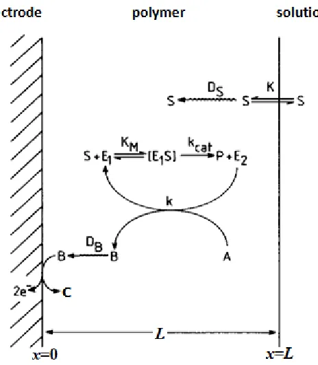
Eq. (1) gives the reduction of the enzyme from E1 to E2. In this reaction scheme, the

[image:3.596.188.420.238.504.2]

re-oxidation of the enzyme reacts with oxygen (A) producing hydrogen peroxide (B), and then B which reacts at a microparticle with a pseudo first-order rate constant (k) producing water (C).

Figure 1. Schematic diagram of possible mechanisms occurring at an enzyme electrode.

A general scheme (Fig. 1) that represents the reaction occurring at a microparticle is shown below:

B E A

E 1

k 2

e

 

 (2)

C 2

B

k

  

e ₍₃₎

At steady-state mass balances within the film for the above enzymatic reaction, leads to the following system of non-linear differential equations [20]:

0

2 2

  

s K

se k dx

s d D

M cat S



(4)

0

2 2

   

s K

se k kb dx

b d D

M cat B



(5)

Atx 0, ds 0, b 0

dx

   (6)

At xL s, k s_{s }, b0

(7)

Where x stands for space, s(x) and b(x) denote the concentration functions of the substrate and, hydrogen peroxide respectively. e_ is the total enzyme concentration in the film



e_ e₁e₂



, D_S is the diffusion coefficient of substrate into polymer film, D_B is the diffusion coefficient of hydrogen peroxide into polymer film, K_M is the Michaelis-Menten constant, kcat is the catalytic reaction rate

constant, ks is the partition coefficient of substrate in the film,L is film thickness, k is the change transfer rate constant for oxidation of hydrogen peroxide and s_ denotes concentration of substrate in the bulk solution. The flux of hydrogen peroxide reacting at the electrode surface is

0

b B

x

db

j D

dx _

   _{ }

  (8)

2.2. Normalized form

The governing differential equations are non-dimensionalized using the following appropriate normalizing parameters.

1 ₁

2 ₂

1

; ; ; S M ; B ; ; ; s

s b

s s cat s b M

D K D k s

s b x L L

u v X

k s k s L  k e_  k      K



 

  _{ }

   _{ } _{ }   

 

  (9

Using the above normalizing parameters, the equations (4) and (5) can be written as follows:

2 2

2 0

1

d u u

dX u

 

 

 (10)

2

2 2

1

2 0

1

d v u

v

dX u

 



  

 (11)

Where _s is the kinetic length of the substrate and _b is the kinetic length of the hydrogen peroxide and u and v represent the normalised concentrations of substrate and hydrogen peroxide. The boundary conditions in non-dimensional form for the studied cases are:

whenX 0, du 0, v 0

dX

  

(12)

whenX 1, u1, v0 ₍₁₃₎ The normalised flux is expressed as,

0

b

X B s

j L dv

D k s dX



 

   _{  }

  (14)

3. ANALYTICAL EXPRESSION OF THE CONCENTRATION AND FLUX USING NEW HOMOTOPY APPROACH

 

0( ) cosh sec

1 1

u X u X  X h 

 

   

  _ _ _ _

 

    (15)

 







2



_{ }





 

 

1 1

2

0 _{2 1} 1

1

cosh

sinh (1 ) sinh 1

( )

sinh 1

sinh cosh cosh

1 1

X

X X

v X v X



  _





 

   _

 

  

 _ _ _



  

  _   _

   

  _{ }

   

   

 _  _{ }  _ 

 

(16)

Using Eq. (14), we can obtain the normalised flux as follows:







2



 

 

2 1

1 1

2 1 cos coth sec ₁

1

ech h

  

  

   

  

   _ _



    

(17)

Eq. (15) and Eq. (16) represent the new simple analytical expression of the concentrations of the substrate and hydrogen peroxide for all values of parameters  , 1 and . Eq. (17) is the simple analytical expression of normalised flux for all values of parameters  , 1 and  .

[image:5.596.89.508.378.687.2]

4. NUMERICAL SIMULATION

Figure 2. Normalized concentration profiles of substrate calculated from Eq. (15), for different values

of 1

; ;

[image:6.596.73.515.74.426.2]

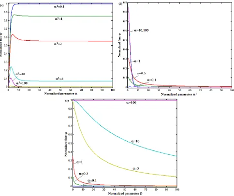
Figure 3. Normalized concentration profiles of hydrogen peroxide calculated from Eq. (16) when (a)

1

0.1; 0.1

    , (b)  0.1;  0.1 and (c) 0.1;10.1. Solid lines represent the analytical solution obtained in this work; dotted lines represent the numerical solution.

The function pdex4 in Matlab/Scilab software which is a function of solving the initial boundary value problems for parabolic-elliptic partial differential equations is used to solve the equation (10) and (11).

Figures 2-4 illustrate the comparison of analytical result obtained in this work with the numerical result. Upon comparison, it is evident that both the results give satisfactory agreement. The Matlab/Scilab program is also given in Appendix -B.

5. DISCUSSION

Figs. 2-4 show the normalized concentration profiles of substrate and hydrogen peroxide in the film which are calculated from Eqs. (15) and (16) respectively. The distributions of substrate and hydrogen peroxide are shown to be dependent on the value of kinetic length

1

/ _s and / _b

L L

Figure 4. Plot of the normalized concentration profiles for hydrogen peroxide for various values of (a) normalised film thickness, L/_s, (b) the normalised film thickness, L/_b, and (c) the normalised parameter . The curves are calculated from Eq. (16).

Concentration profiles in the film may be helpful to understand the present model in detail. Figs. 2(a)-(c) represent the concentration profiles of the substrate for various values of the parameters

and

 . From figures 2(a)-(b), it is inferred that the value of the concentration u increases when / s

L

  decreases. Concentration of the substrate is uniform when L/s 0.5or width of the film is small. For small value of L/s, substrate diffuses into the electrode surface.

[image:7.596.60.535.69.444.2]

Figure 5. Plot of the normalised flux,  , against (a) the normalised parameter and (b) the normalised parameter 1 and (c) the normalised parameter . The curves are calculated from Eq. (17).

The normalized flux  is plotted in Figs. 5(a)-(c). It illustrates that the flux for all values of

1

/ _s and / _b

L L

     . In fig. 5(a), the flux increases when the parameter 1 decreases. The flux reaches the steady state value when L/_s20, for all values of 1L/_b. From fig. 5(b), it is observed that the flux increases as  increases and when 120, all the curves reach the steady state value. From fig. 5(c), it is known that the flux increases when  increases.

Recently Anitha et.al [22] studied a theoretical model for an amperometric enzyme electrodes based on an immobilized flavoprotein. When DS DB,and 0

1 





b 



, Anitha et.al [22]

obtained the analytical expression for the concentration of substrate and hydrogen peroxide as follows:

 

 

_{ }



 









 



 





 

3

cosh 6

2 cosh 3 cosh 2

cosh 3 cosh cosh

cosh



 

 

 

 _   

 X X X

X u

[image:8.596.55.539.68.472.2]

 

 







 







 

 







 



 











 

 







 

3

cosh 6 3 2 cosh cosh 2 2 cosh 1 cosh 1 cosh 2 cosh 3 cosh cosh 1 cosh 1            X X X X X X v             (19)

The expression of the normalized current becomes

 



 

 



 

3

cosh 6 2 cosh cosh 2 3 sec 1     

   h   

(20)

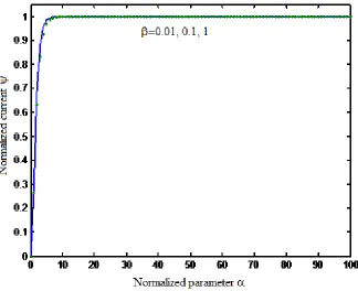
The normalized current  _{in previous work (Eqn.(20)) is compared with our present work}

[image:9.596.135.459.339.603.2]

(Eq. (17)) in Figure-6 for  1 and 1 0.01

.

From this figure, we conclude that the numerical value of current reported in previous work [22] ( Eq. (20)) and our work Eq. (17) are same. From this figure, it is obvious that the values of the current reach the maximum value 1.

Figure 6. Plot of normalized current  versus at mixed oxidase enzyme for  1 when 1 0.01. Symbols: (—)Eq. (20); ( )Eq. (17). Solid lines are compared with points.

6. CONCLUSION

kinetics of the amperometric biosensor. This theoretical results will be used to investigate the biosensor response and current by altering this model parameters which influencing the enzyme kinetics as well as the mass transport by diffusion. Our study helps future researchers in better understanding of the application of an amperometric biosensor in suitable phase with the help of mathematical analysis.

ACKNOWLEDGEMENT

This work was supported by the Council of Scientific and Industrial Research (CSIR) Ref No. 01(2442)/10/EMR-II, Government of India. The authors also thank the secretary, The Madura College Board, and the principal, The Madura College, Madurai, Tamil Nadu, India, for their support and encouragement.

Appendix A:

Approximate analytical solution of the concentrations of the substrate and hydrogen peroxide using new Homotopy perturbation method.In this appendix, solution of non-linear system of equations (Eq. (10) and Eq. (11)) is derived using new Homotopy perturbation method.

`













2 2 2 2

(1 ) " " 0

1 1

d u u

p p u uu u

dX u X

 _{ }       _  _       

  ` (A.1)













2 2 2

2 2

1 1 2 1

2

(1 ) " " 0

1 1

d v u

p v p v uv uv u v

dX u X

             _   _         

  (A.2)

Supposing the approximate solutions of Eq. (A.1) and Eq. (A.2) have the form

            .. ... .. ... 2 2 1 0 2 2 1 0 v p pv v v u p pu u u (A.3)

Substituting Eq. (A.3) into Eq. (A.1) and Eq. (A.2) (respectively), and equate the terms with the identical powers of p, we obtain





2 2

0 0 0

2

: 0

1

d u u p

dX

 

 

 (A.4)









2 2

2 2

1 1 1 0 0 2

0 0

2 2

: 0

1 1

d u u

d u u

p u u

dX dX



 _{ }

 

    

  (A.5) and





2

2 2

0 0 1 0

0 2

: 0

1

d v u

p v dX      

 (A.6)



 



2 2 2 2

2 2

1 1 1 0 0 1 1 2

1 0 0 0 0

2 2

: 0

1 1

d v u

d v u

p v u u v u

dX dX

 

   

 

      

  (A.7)

The initial conditions are as follows: 0

) 0 (

0 X  dX 

du ; u0(X 1)1 (A.8)

0( 0) 0

v X   ; v X0(  1) 0 (A.9)

and

0 )

0

(X  dX 

( 0) 0

i

v X   ; v_i(X 1)0for all i=1,2,3,… (A.11)

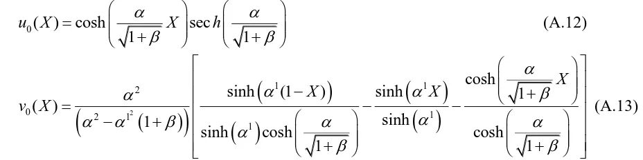
Solving the Eq. (A.4) and Eq. (A.6) and using the boundary conditions Eq. (A.8) and Eq. (A.9), we get

0( ) cosh sec

1 1

u X  X h 

 

   

 _ _ _ _

 

    (A.12)







2



_{ }





 

 

1 1

2

0 _{2 1 1}

1

cosh

sinh (1 ) sinh 1

( )

sinh 1

sinh cosh cosh

1 1

X

X X

v X



  





 

   _

 

  

 _ _ _



  

 _   _

   

  _{ }

   

   

 _  _{ }  _ 

 

(A.13)

Substituting the value of u₀

 

X in the Eq. (A.5) and solving the equations, using the boundary condition Eq. (A.10), we can obtain the value of u X₁

 

. Similarly we can get the value of v₁

 

X by solving the Eq. (A.7). When p=1, the approximate solution Eq. (A.3) becomes

0 1 0

( )

u X u  u u (A.14)

0 1 0

( )

v X   v v v

(A.15) Using the above equations, we get equations. (15) and . (16) in the next.

Appendix B:

Matlab/Scilab program to find the numerical solution of equations (10)–(11) function

m = 0;

x = linspace(0,1); t = linspace(0,100);

sol = pdepe(m,@pdex4pde,@pdex4ic,@pdex4bc,x,t); u1 = sol(:,:,1);

[image:11.596.74.538.125.241.2]

u2 = sol(:,:,2); figure

plot(x,u1(end,:)) title('Solution at t = 2') xlabel('Distance x') ylabel('u1(x,2)') figure

plot(x,u2(end,:)) title('Solution at t = 2') xlabel('Distance x') ylabel('u2(x,2)')

% --- function [c,f,s] = pdex4pde(x,t,u,DuDx);

alpha=1; beta=1;

c = [1;1]; f = [1; 1] .* DuDx;

F1 =-u(1)/(h^2*(1+alpha*u(1)));

F2 =-u(2)/(h1^2)+beta*u(1)/(h^2*(1+alpha*u(1))); s =[F1; F2];

% --- function u0 = pdex4ic(x);

u0 = [1; 0];

% --- function [pl,ql;pr;qr] = pdex4bc(xl,ul,xr,ur,t);

pl = [0; 0]; ql = [1; 1];

pr = [ur(1)-1; ur(2)-1]; qr = [0; 0];

References

1. R. W. Cattrall, In Chemical Sensors, Oxford University Press, Oxford, 1997.

2. F. W. Scheller, D. Pfeiffer, F. Schubert, R. Rermeberg and D. Kirstein, Biosensors, Fundamentals and Applications, in A. P. F. Turner, I. Karube and G. S. Wilson (Eds.), Oxford University Press, Oxford, 1987, 318.

3. D. A. Johnson, M. F. Cardosi and D. H. Vaughan, Electroanalysis, 7 (1995) 520.

4. V. G. Prabhu, L. R. Zarapkar and R. G. Dhaneshwar, Electrochim. Acta, 26 (1981) 725. 5. J. Wang, J. Liu and F. Lu, Anal. Chem., 66 (1994) 3600.

6. H. Sakslund, J. Wang, F. Lu and O. Hammerich, J. Electroanal.Chem., 397 (1995) 149.

7. J. Wang, F. Lu, L. Agnes, J. Liu, H. Saksland, Q. Chen, M. Pedrero, L. Chen and O. Hammerich, Anal. Chim. Acta, 305 (1995) 3.

8. M. Somasundrum, M. Tanticharoen and K. Kirtikara, J. Electroanal. Chem., 407 (1996) 247. 9. D. Bootkul, P. Taotong, M. Somasundrum, K. Kirtikara and M. Tanticharoen, Proc. 4th World

Congress on Biosensors, Bangkok, 29-31 May, 1995, 205. 10. M. E. G. Lyons, Analyst, 119 (1994) 805.

11. P. N. Bartlett and R. G. Whitaker, J. Electroanal. Chem., 224 (1987) 27.

12. M. E. G. Lyons, D. E. McCormack and P. N. Bartlett, J. Electroanal. Chem., 261 (1989) 51. 13. J. Wang, G. Rivas and M. Chicharro, Electroanalysis, 8 (1996) 434.

14. J. Wang, L. Chen, L. Liu and F. Lu, Electroanalysis, 8 (1996) 1127.

15. M. R. Romero, A. M. Baruzzi and F. Garay, Sensors and Actuators B: Chemical, 162 (2012) 284. 16. I. Iliev, P. Atanasov, S. Gamburzev, A. Kaisheva and V. Tonchev, Sensors and Actuators B:

Chemical,8 (1992) 65.

17. A. Bergel and M. Comtat, Anal. Chem., 56 (1984) 2904.

18. R. Baronas, F. Ivanauskas and J. Kulys, Sensors, 3 (2003) 248. 19. P. Gros and A. Bergel, J. Electroanal. Chem., 386 (1995) 65.

21. L. Rajendran and S. Anitha, Electrochim. Acta, 102 (2013) 474.

22. S. Anitha, A. Subbiah, S. Subramaniam and L. Rajendran, Electrochim.Acta, 56 (2011) 3345.