#8 pdf

Chapter 7

AdaBoost

Zhi-Hua Zhou and Yang Yu

Contents

7.1 Introduction . . . .127

7.2 The Algorithm . . . .128

7.2.1 Notations . . . .128

7.2.2 A General Boosting Procedure . . . .129

7.2.3 The AdaBoost Algorithm . . . .130

7.3 Illustrative Examples . . . .133

7.3.1 Solving XOR Problem . . . .133

7.3.2 Performance on Real Data . . . .134

7.4 Real Application . . . .136

7.5 Advanced Topics. . . .138

7.5.1 Theoretical Issues. . . .138

7.5.2 Multiclass AdaBoost . . . .142

7.5.3 Other Advanced Topics . . . .145

7.6 Software Implementations. . . .145

7.7 Exercises . . . .146

References . . . .147

7.1

Introduction

slightly better than random guess, to strong learners, which can make very accurate predictions. So, “base learners” are also referred as “weak learners.”

AdaBoost [9, 10] is one of the most influential ensemble methods. It took birth from the answer to an interesting question posed by Kearns and Valiant in 1988. That is, whether two complexity classes, weakly learnable and strongly learnable prob-lems, are equal. If the answer to the question is positive, a weak learner that performs just slightly better than random guess can be “boosted” into an arbitrarily accurate strong learner. Obviously, such a question is of great importance to machine learning. Schapire [21] found that the answer to the question is “yes,” and gave a proof by construction, which is the first boosting algorithm. An important practical deficiency of this algorithm is the requirement that the error bound of the base learners be known ahead of time, which is usually unknown in practice. Freund and Schapire [9] then pro-posed an adaptive boosting algorithm, named AdaBoost, which does not require those unavailable information. It is evident that AdaBoost was born with theoretical signif-icance, which has given rise to abundant research on theoretical aspects of ensemble methods in communities of machine learning and statistics. It is worth mentioning that for their AdaBoost paper [9], Schapire and Freund won the Godel Prize, which is one of the most prestigious awards in theoretical computer science, in the year 2003. AdaBoost and its variants have been applied to diverse domains with great success, owing to their solid theoretical foundation, accurate prediction, and great simplicity (Schapire said it needs only “just 10 lines of code”). For example, Viola and Jones [27] combined AdaBoost with a cascade process for face detection. They regarded rectan-gular features as weak learners, and by using AdaBoost to weight the weak learners, they got very intuitive features for face detection. In order to get high accuracy as well as high efficiency, they used a cascade process (which is beyond the scope of this chap-ter). As a result, they reported a very strong face detector: On a 466 MHz machine, face

detection on a 384×288 image costs only 0.067 second, which is 15 times faster than

state-of-the-art face detectors at that time but with comparable accuracy. This face detector has been recognized as one of the most exciting breakthroughs in computer vision (in particular, face detection) during the past decade. It is not strange that “boost-ing” has become a buzzword in computer vision and many other application areas.

In the rest of this chapter, we will introduce the algorithm and implementations, and give some illustrations on how the algorithm works. For readers who are eager to know more, we will introduce some theoretical results and extensions as advanced topics.

7.2

The Algorithm

7.2.1

Notations

We first introduce some notations that will be used in the rest of the chapter. LetX

denote the instance space, or in other words, feature space. LetY denote the set of

7.2 The Algorithm 129

letY = {−1,+1}for binary classification. A training set D consists of m instances

whose associated labels are observed, i.e., D = {(xi,yi)}(i ∈ {1, . . . ,m}), while

the label of a test instance is unknown and thus to be predicted. We assume both training and test instances are drawn independently and identically from an underlying

distributionD.

After training on a training data set D, a learning algorithmLwill output a

hypoth-esis h, which is a mapping fromXtoY, or called as a classifier. The learning process

can be regarded as picking the best hypothesis from a hypothesis space, where the word “best” refers to a loss function. For classification, the loss function can naturally be 0/1-loss,

loss0/1(h|x)=I[h(x)=y]

whereI[·] is the indication function which outputs 1 if the inner expression is true

and 0 otherwise, which means that one error is counted if an instance is wrongly classified. In this chapter 0/1-loss is used by default, but it is noteworthy that other kinds of loss functions can also be used in boosting.

7.2.2

A General Boosting Procedure

Boosting is actually a family of algorithms, among which the AdaBoost algorithm is the most influential one. So, it may be easier by starting from a general boosting procedure.

Suppose we are dealing with a binary classification problem, that is, we are trying to classify instances as positive and negative. Usually we assume that there exists an unknown target concept, which correctly assigns “positive” labels to instances belonging to the concept and “negative” labels to others. This unknown target concept is actually what we want to learn. We call this target concept ground-truth. For a binary classification problem, a classifier working by random guess will have 50% 0/1-loss. Suppose we are unlucky and only have a weak classifier at hand, which is only

slightly better than random guess on the underlying instance distributionD, say, it

has 49% 0/1-loss. Let’s denote this weak classifier as h1. It is obvious that h1is not

what we want, and we will try to improve it. A natural idea is to correct the mistakes

made by h1.

We can try to derive a new distributionDfromD, which makes the mistakes of

h1more evident, for example, it focuses more on the instances wrongly classified by

h1(we will explain how to generateDin the next section). We can train a classifier

h2 fromD. Again, suppose we are unlucky and h2is also a weak classifier. Since

D _{was derived fromD, ifD satisfies some condition, h}

2 will be able to achieve

a better performance than h1 on some places inD where h1 does not work well,

without scarifying the places where h1 performs well. Thus, by combining h1 and

h2in an appropriate way (we will explain how to combine them in the next section),

the combined classifier will be able to achieve less loss than that achieved by h1. By

repeating the above process, we can expect to get a combined classifier which has

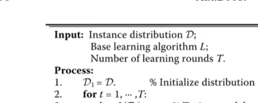
Input: Instance distribution D; Base learning algorithm L; Number of learning rounds T.

Process:

1. D1 = D. % Initialize distribution

2. for t = 1, ··· ,T:

3. ht = L(Dt); % Train a weak learner from distribution Dt

4. єt = Prx~Dt ,yI[ht (x)≠ y]; % Measure the error of ht

5. Dt+1= AdjustDistribution (Dt , єt)

6. end

Output: H(x) = CombineOutputs({ht(x)})

Figure 7.1 A general boosting procedure.

Briefly, boosting works by training a set of classifiers sequentially and combining them for prediction, where the later classifiers focus more on the mistakes of the earlier classifiers. Figure 7.1 summarizes the general boosting procedure.

7.2.3

The AdaBoost Algorithm

Figure 7.1 is not a real algorithm since there are some undecided parts such as Ad j ust Di str i buti on and Combi neOut puts. The AdaBoost algorithm can be viewed as an instantiation of the general boosting procedure, which is summarized in Figure 7.2.

Input: Data set D = {(x1, y1), (x2, y2), . . . , (xm, ym)}; Base learning algorithm L;

Number of learning rounds T.

Process:

1. D1 (i) = 1/m. % Initialize the weight distribution

2. for t = 1, ··· ,T:

3. ht = L(D, Dt); % Train a learner ht from Dusing distribution Dt

4. єt = Prx~Dt ,yI[ht (x)≠ y]; % Measure the error of ht

5. ifєt > 0.5 then break

6. αt = ½ ln

(

)

7. Dt+1(i) =

8. end

Output: H(x) = sign (Σt=1αt ht(x))

×

{

exp(αt) if ht(xi) ≠ yi

% Update the distribution, where

% Zt is a normalization factor which

% enables Dt+1 to be distribution

T 1– єt

єt Dt(i)

Zt

Dt(i)exp(–αt yi ht (xi))

Zt

7.2 The Algorithm 131

Now we explain the details.1 _{AdaBoost generates a sequence of hypotheses and}

combines them with weights, which can be regarded as an additive weighted combi-nation in the form of

H (x)=

T

t=1

αtht(x)

From this view, AdaBoost actually solves two problems, that is, how to generate the

hypotheses ht’s and how to determine the proper weightsαt’s.

In order to have a highly efficient error reduction process, we try to minimize an exponential loss

lossexp(h)=Ex∼D,y[e−yh(x)]

where yh(x) is called as the classification margin of the hypothesis.

Let’s consider one round in the boosting process. Suppose a set of hypotheses as well as their weights have already been obtained, and let H denote the combined hypothesis. Now, one more hypothesis h will be generated and is to be combined

with H to form H+αh. The loss after the combination will be

lossexp(H+αh)=Ex∼D,y[e−y(H (x)+αh(x))]

The loss can be decomposed to each instance, which is called pointwise loss, as

lossexp(H+αh |x)=Ey[e−y(H (x)+αh(x))|x]

Since y and h(x) must be+1 or−1, we can expand the expectation as

lossexp(H+αh |x)=e−y H (x)

e−αP(y=h(x)|x)+eαP(y=h(x)|x)

Suppose we have already generated h, and thus the weightαthat minimizes the

loss can be found when the derivative of the loss equals zero, that is,

∂lossexp(H+αh |x)

∂α =e−y H (x)

−e−α_{P(y=h(x)|x)+e}α_P(y=h(x)|x)

=0

and the solution is

α= 1

2ln

P(y=h(x)|x)

P(y=h(x)|x) = 1 2ln

1−P(y=h(x)|x)

P(y=h(x)|x)

By taking an expectation overx, that is, solving ∂lossexp(H+αh)

∂α =0, and denoting

=Ex∼D[y=h(x)], we get

α=1

2ln

1−

which is the way of determiningαt in AdaBoost.

1_{Here we explain the AdaBoost algorithm from the view of [11] since it is easier to understand than the}

Now let’s consider how to generate h. Given a base learning algorithm, AdaBoost invokes it to produce a hypothesis from a particular instance distribution. So, we only need to consider what hypothesis is desired for the next round, and then generate an instance distribution to achieve this hypothesis.

We can expand the pointwise loss to second order about h(x) =0, when fixing

α=1,

lossexp(H+h|x)≈Ey[e−y H (x)(1−yh(x)+y2h(x)2/2)|x]

=Ey[e−y H (x)(1−yh(x)+1/2)|x]

since y2_{=1 and h(x)}2_=1.

Then a perfect hypothesis is

h∗(x)=arg min

h

lossexp(H+h|x)=arg max

h

Ey[e−y H (x)yh(x)|x]

=arg max

h

e−H (x)P(y=1|x)·1·h(x)+eH (x)P(y= −1|x)·(−1)·h(x)

Note thate−y H (x)_{is a constant in terms of h(x). By normalizing the expectation as}

h∗(x)=arg max

h

e−H (x)_{P(y=1|x)·1·h(x)+e}H (x)_{P(y= −1|x)·(−1)·h(x)} e−H (x)_P(y=1|x)+eH (x)_{P(y= −1|x)}

we can rewrite the expectation using a new term w(x,y), which is drawn from

e−y H (x)_{P(y|x), as}

h∗(x)=arg max

h

Ew(x,y)∼e−y H (x)_P(y|x)[yh(x)|x]

Since h∗(x) must be+1 or−1, the solution to the optimization is that h∗(x) holds

the same sign with y|x, that is,

h∗(x)=Ew(x,y)∼e−y H (x)_P(y|x₎[y|x]

=P_w(x,y)∼e−y H (x)_P(y|x)(y=1|x)−P_w(x,y)∼e−y H (x)_P(y|x)(y= −1|x)

As can be seen, h∗simply performs the optimal classification ofxunder the

distri-bution e−y H (x)_{P(y |x). Therefore, e}−y H (x)_{P(y|x) is the desired distribution for a}

hypothesis minimizing 0/1-loss.

So, when the hypothesis h(x) has been learned andα= 1₂ln1− has been

deter-mined in the current round, the distribution for the next round should be

Dt₊1(x)=e−y(H (x)+αh(x))P(y|x)=e−y H (x)P(y|x)·e−αyh(x) =Dt(x)·e−αyh(x)

which is the way of updating instance distribution in AdaBoost.

But, why optimizing the exponential loss works for minimizing the 0/1-loss? Actually, we can see that

h∗(x)=arg min

h E

x∼D,y[e−yh(x) |x]=

1

2ln

P(y=1|x)

7.3 Illustrative Examples 133

and therefore we have

sign(h∗(x))=arg max

y P(y|x)

which implies that the optimal solution to the exponential loss achieves the minimum Bayesian error for the classification problem. Moreover, we can see that the function

h∗which minimizes the exponential loss is the logistic regression model up to a factor

2. So, by ignoring the factor 1/2, AdaBoost can also be viewed as fitting an additive

logistic regression model.

It is noteworthy that the data distribution is not known in practice, and the AdaBoost algorithm works on a given training set with finite training examples. Therefore, all the expectations in the above derivations are taken on the training examples, and the weights are also imposed on training examples. For base learning algorithms that cannot handle weighted training examples, a resampling mechanism, which samples training examples according to desired weights, can be used instead.

7.3

Illustrative Examples

In this section, we demonstrate how the AdaBoost algorithm works, from an illustra-tion on a toy problem to real data sets.

7.3.1

Solving XOR Problem

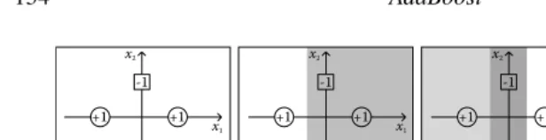
We consider an artificial data set in a two-dimensional space, plotted in Figure 7.3(a). There are only four instances, that is,

⎧ ⎪ ⎪ ⎪ ⎨ ⎪ ⎪ ⎪ ⎩

(x1=(0,+1),y1= +1)

(x2=(0,−1),y2= +1)

(x3=(+1,0),y3= −1)

(x4=(−1,0),y4= −1)

⎫ ⎪ ⎪ ⎪ ⎬ ⎪ ⎪ ⎪ ⎭

This is the XOR problem. The two classes cannot be separated by a linear classifier which corresponds to a line on the figure.

Suppose we have a base learning algorithm which tries to select the best of the fol-lowing eight functions. Note that none of them is perfect. For equally good functions, the base learning algorithm will pick one function from them randomly.

h1(x)=

+1, if (x1>−0.5)

−1, otherwise h2(x)=

−1, if (x1>−0.5)

+1, otherwise

h3(x)=

+1, if (x1>+0.5)

−1, otherwise h4(x)=

−1, if (x1>+0.5)

(a) The XOR data (b) 1st round (c) 2nd round (d) 3rd round +1 +1 -1 -1 +1 +1 -1 -1 x2 x1 x2 x1 +1 +1 -1 -1 x2 x1 -0.55

0.55 -0.25-1.350.25

+1 +1 -1 -1 x2 x1 -2.45 -1.350.85-0.25-0.851.35

Figure 7.3 AdaBoost on the XOR problem.

h5(x)=

+1, if (x2>−0.5)

−1, otherwise h6(x)=

−1, if (x2>−0.5)

+1, otherwise

h7(x)=

+1, if (x2>+0.5)

−1, otherwise h8(x)=

−1, if (x2>+0.5)

+1, otherwise

where x1and x2are the values ofxat the first and second dimension, respectively.

Now we track how AdaBoost works:

1. The first step is to invoke the base learning algorithm on the original data. h2,

h3, h5, and h8all have 0.25 classification errors. Suppose h2is picked as the first

base learner. One instance,x1, is wrongly classified, so the error is 1/4=0.25.

The weight of h2is 0.5 ln 3≈0.55. Figure 7.3(b) visualizes the classification,

where the shadowed area is classified as negative (−1) and the weights of the

classification, 0.55 and−0.55, are displayed.

2. The weight ofx1is increased and the base learning algorithm is invoked again.

This time h3, h5, and h8 have equal errors. Suppose h3 is picked, of which

the weight is 0.80. Figure 7.3(c) shows the combined classification of h2 and

h3with their weights, where different gray levels are used for distinguishing

negative areas according to classification weights.

3. The weight ofx3is increased, and this time only h5 and h8equally have the

lowest errors. Suppose h5is picked, of which the weight is 1.10. Figure 7.3(d)

shows the combined classification of h2, h3, and h8. If we look at the sign of

classification weights in each area in Figure 7.3(d), all the instances are correctly classified. Thus, by combining the imperfect linear classifiers, AdaBoost has produced a nonlinear classifier which has zero error.

7.3.2

Performance on Real Data

We evaluate the AdaBoost algorithm on 56 data sets from the UCI Machine Learning

Repository,2_{which covers a broad range of real-world tasks. We use the Weka (will be}

introduced in Section 7.6) implementation of AdaBoost.M1 using reweighting with

7.3 Illustrative Examples 135

AdaBoost with decision tree (unpruned)

AdaBoost with decision tree (pruned) AdaBoost with decision stump

Decision stump

Decision tree (pruned)

1.00

0.80

0.60

0.40

0.20

0.00

1.00

0.80

0.60

0.40

0.20

0.00

0.00 0.20 0.40 0.60 0.80 1.00 0.00 0.20 0.40 0.60 0.80 1.00

Decision tree (unpruned)

1.00

0.80

0.60

0.40

0.20

0.00

0.00 0.20 0.40 0.60 0.80 1.00

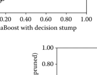
Figure 7.4 Comparison of predictive errors of AdaBoost against decision stump, pruned, and unpruned single decision trees on 56 UCI data sets.

50 base learners. Almost all kinds of learning algorithms can be taken as base learning algorithms, such as decision trees, neural networks, and so on. Here, we have tried three base learning algorithms, including decision stump, pruned, and unpruned J4.8 decision trees (Weka implementation of C4.5).

We plot the comparison results in Figure 7.4, where each circle represents a data set and locates according to the predictive errors of the two compared algorithms. In each plot of Figure 7.4, the diagonal line indicates where the two compared algorithms have identical errors. It can be observed that AdaBoost often outperforms its base learning algorithm, with a few exceptions on which it degenerates the performance.

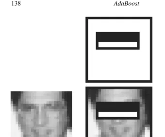
Figure 7.5 Four feature masks to be applied to each rectangle.

7.4

Real Application

Viola and Jones [27] combined AdaBoost with a cascade process for face detection.

As the result, they reported that on a 466 MHz machine, face detection on a 384×288

image costs only 0.067 seconds, which is almost 15 times faster than state-of-the-art face detectors at that time but with comparable accuracy. This face detector has been recognized as one of the most exciting breakthroughs in computer vision (in particular, face detection) during the past decade. In this section, we briefly introduce how AdaBoost works in the Viola-Jones face detector.

Here the task is to locate all possible human faces in a given image. An image is

first divided into subimages, say 24×24 squares. Each subimage is then represented

by a feature vector. To make the computational process efficient, very simple features are used. All possible rectangles in a subimage are examined. On every rectangle, four features are extracted using the masks shown in Figure 7.5. With each mask, the sum of pixels’ gray level in white areas is subtracted by the sum of those in dark

areas, which is regarded as a feature. Thus, by a 24×24 splitting, there are more than

1 million features, but each of the features can be calculated very fast. Each feature is regarded as a weak learner, that is,

hi_,p_,θ(x)=I[ pxi ≤ pθ] ( p∈ {+1,−1})

where xiis the value ofxat the i -th feature.

The base learning algorithm tries to find the best weak classifier hi∗,p∗,θ∗ that

minimizes the classification error, that is,

(i∗,p∗, θ∗)=arg min

i,p,θ

E(x,y)I[hi_,p_,θ(x)=y]

Face rectangles are regarded as positive examples, as shown in Figure 7.6, while rectangles that do not contain any face are regarded as negative examples. Then, the AdaBoost process is applied and it will return a few weak learners, each corresponds to one of the over 1 million features. Actually, the AdaBoost process can be regarded as a feature selection tool here.

7.4 Real Application 137

Figure 7.6 Positive training examples [27].

the second feature measures how the intensity of the two eye areas differ from the area between two eyes.

Using the selected features in order, an extremely imbalanced decision tree is built, which is called cascade of classifiers, as illustrated in Figure 7.8.

The parameterθis adjusted in the cascade such that, at each tree node, branching

Figure 7.7 Selected features [27].

7.5

Advanced Topics

7.5.1

Theoretical Issues

Computational learning theory studies some fundamental theoretical issues of

machine learning. First introduced by Valiant in 1984 [25], the Probably

Approx-imately Correct (PAC) framework models learning algorithms in a distribution free

manner. Roughly speaking, for binary classification, a problem is learnable or strongly

learnable if there exists an algorithm that outputs a hypothesis h in polynomial time

not a face

face not a face

not a face ...

7.5 Advanced Topics 139

Figure 7.9 Outputs of the Viola-Jones face detector on a number of test images [27].

such that for all 0< δ, ≤0.5,

PEx∼D,y[I[h(x)=y]]<

≥1−δ

and a problem is weakly learnable if the above holds for all 0 < δ ≤ 0.5 but only

whenis slightly smaller than 0.5 (or in other words, h is only slightly better than

random guess).

boosting algorithm. One year later, Freund [7] developed a more efficient algorithm. Both algorithms, however, suffered from the practical deficiency that the error bound of the base learners need to be known ahead of time, which is usually unknown in practice. Later, in 1995, Freund and Schapire [9] developed the AdaBoost algorithm, which is effective and efficient in practice.

Freund and Schapire [9] proved that, if the base learners of AdaBoost have errors 1,2,· · ·,T, the error of the final combined learner,, is upper bounded as

=Ex∼D,yI[H (x)=y]≤2T T

t=1

t(1−t)≤e−2

T t=1γt2

whereγt =0.5−t. It can be seen that AdaBoost reduces the error exponentially

fast. Also, it can be derived that, to achieve an error less than, the round T is upper

bounded as

T ≤

1 2γ2 ln

1

where it is assumed thatγ =γ1=γ2= · · · =γT.

In practice, however, all the operations of AdaBoost can only be carried out on training data D, that is,

D=Ex∼D,yI[H (x)=y]

and thus the errors are training errors, while the generalization error, that is, the error

over instance distributionD

D=Ex∼D,yI[H (x)=y]

is of more interest.

The initial analysis [9] showed that the generalization error of AdaBoost is upper bounded as

D ≤D+O˜

d T m

with probability at least 1−δ, where d is the VC-dimension of base learners, m is

the number of training instances, and ˜O(·) is used instead of O(·) to hide logarithmic

terms and constant factors.

The above bound suggests that in order to achieve a good generalization ability, it is necessary to constrain the complexity of base learners as well as the number of learning rounds; otherwise AdaBoost will overfit. However, empirical studies show that AdaBoost often does not overfit, that is, its test error often tends to decrease even after the training error reaches zero, even after a large number of rounds, such as 1000.

For example, Schapire et al. [22] plotted the performance of AdaBoost on the

letter data set from UCI Machine Learning Repository, as shown in Figure 7.10 (left),

7.5 Advanced Topics 141

er

ror ra

te

ra

tio of t

est s

et

t θ

20

15

10

5

0

1.0

0.5

10 100 1000 -1 -0.5 0.5 1

Figure 7.10 Training and test error (left) and margin distribution (right) of AdaBoost on the letter data set [22].

Razor, that is, nothing more than necessary should be done, which is one of the basic principles in machine learning.

Many researchers have studied this phenomena, and several theoretical explana-tions have been given, for example, [11]. Schapire et al. [22] introduced the margin-based explanation. They argued that AdaBoost is able to increase the margin even after the training error reaches zero, and thus it does not overfit even after a large

number of rounds. The classification margin of h onxis defined as yh(x), and that

of H (x)=tT=1αtht(x) is defined as

y H (x)=

T

t=1αtyht(x)

T

t=1αt

Figure 7.10 (right) plots the distribution of y H (x)≤θfor different values ofθ. It

was proved in [22] that the generalization error is upper bounded as

D≤ Px_∼D,y(y H (x)≤θ)+O˜

d mθ2 +ln

1 δ

≤2T

T

t=1

1−θ

t (1−)1+θ+O˜

d mθ2 +ln

1 δ

with probability at least 1−δ. This bound qualitatively explains that when other

variables in the bound are fixed, the larger the margin, the smaller the generalization error.

However, this margin-based explanation was challenged by Brieman [4]. Using

minimum margin,

=min

x∈Dy H (x)

updatingαtaccording to

αt=

1

2ln

1+γt

1−γt

−1

2ln

1+t

1−t

Interestingly, the minimum margin of arc-gv is uniformly better than that of AdaBoost, but the test error of arc-gv increases drastically on all tested data sets [4]. Thus, the margin theory for AdaBoost was almost sentenced to death.

In 2006, Reyzin and Schapire [20] reported an interesting finding. It is well-known that the bound of the generalization error is associated with margin, the number of rounds, and the complexity of base learners. When comparing arc-gv with AdaBoost, Breiman [4] tried to control the complexity of base learners by using decision trees with the same number of leaves, but Reyzin and Schapire found that these are trees with very different shapes. The trees generated by arc-gv tend to have larger depth, while those generated by AdaBoost tend to have larger width. Figure 7.11 (top) shows the difference of depth of the trees generated by the two algorithms on the

breast cancer data set from UCI Machine Learning Repository. Although the trees

have the same number of leaves, it seems that a deeper tree makes more attribute tests than a wider tree, and therefore they are unlikely to have equal complexity. So, Reyzin and Schapire repeated Breiman’s experiments by using decision stump, which has only one leaf and therefore is with a fixed complexity, and found that the margin distribution of AdaBoost is actually better than that of arc-gv, as illustrated in Figure 7.11 (bottom).

Recently, Wang et al. [28] introduced equilibrium margin and proved a new bound tighter than that obtained by using minimum margin, which suggests that the mini-mum margin may not be crucial for the generalization error of AdaBoost. It will be interesting to develop an algorithm that maximizes equilibrium margin directly, and to see whether the test error of such an algorithm is smaller than that of AdaBoost, which remains an open problem.

7.5.2

Multiclass AdaBoost

In the previous sections we focused on AdaBoost for binary classification, that is,

Y = {+1,−1}. In many classification tasks, however, an instance belongs to one of

many instead of two classes. For example, a handwritten number belongs to 1 of 10

classes, that is,Y= {0, . . . ,9}. There is more than one way to deal with a multiclass

classification problem.

AdaBoost.M1 [9] is a very direct extension, which is as same as the algorithm shown in Figure 7.2, except that now the base learners are multiclass learners instead of binary classifiers. This algorithm could not use binary base classifiers, and requires every

base learner have less than 1/2 multiclass 0/1-loss, which is an overstrong constraint.

SAMME [35] is an improvement over AdaBoost.M1, which replaces Line 5 of AdaBoost.M1 in Figure 7.2 by

αt =

1

2ln

1−t

t

7.5 Advanced Topics 143 C u m u la tive a verage tr ee de pt h C u m u la tive f re quenc y 10 9.5 9 8.5 8 7.5 7 500 0.7 0.6 0.5 0.4 0.3 0.2 0.1 0 -0.1 450 400 350 300 250 200 150 100 50 Round (a) “AdaBoost_bc” “Arc-gv_bc” 1.2 1 0.8 0.6 0.4 0.2 0 “AdaBoost_bc” “Arc-gv_bc” Margin (b)

Figure 7.11 Tree depth (top) and margin distribution (bottom) of AdaBoost against arc-gv on the breast cancer data set [20].

This modification is derived from the minimization of multiclass exponential loss. It was proved that, similar to the case of binary classification, optimizing the multiclass exponential loss approaches to the optimal Bayesian error, that is,

sign[h∗(x)]=arg max

y∈Y

P(y|x)

A popular solution to multiclass classification problem is to decompose the task into multiple binary classification problems. Direct and popular decompositions include

one-vs-rest and one-vs-one. One-vs-rest decomposes a multiclass task of|Y|classes

into |Y| binary classification tasks, where the i -th task is to classify whether an

instance belongs to the i -th class or not. One-vs-one decomposes a multiclass task

of|Y|classes into |Y|(|Y|−₂ 1)binary classification tasks, where each task is to classify

whether an instance belongs to, say, the i -th class or the j -th class.

AdaBoost.MH [23] follows the one-vs-rest approach. After training|Y|number of

(binary) AdaBoost classifiers, the real-value output H (x) =Tt=1αtht(x) of each

AdaBoost is used instead of the crisp classification to find the most probable class, that is,

H (x)=arg max

y_∈Y

Hy(x)

where Hyis the AdaBoost classifier that classifies the y-th class from the rest.

AdaBoost.M2 [9] follows the one-vs-one approach, which minimizes a pseudo-loss. This algorithm is later generalized as AdaBoost.MR [23] which minimizes a ranking loss motivated by the fact that the highest ranked class is more likely to be the correct class. Binary classifiers obtained by one-vs-one decomposition can also be aggregated by voting or pairwise coupling [13].

Error correcting output codes (ECOCs) [6] can also be used to decompose a

multiclass classification problem into a series of binary classification problems. For example, Figure 7.12a shows output codes for four classes using five classifiers. Each

classifier is trained to discriminate the+1 and−1 classes in the corresponding column.

For a test instance, by concatenating the classifications output by the five classifiers, a code vector of predictions is obtained. This vector will be compared with the code vector of the classes (every row in Figure 7.12(a) using Hamming distance, and the class with the shortest distance is deemed the final prediction. According to infor-mation theory, when the binary classifiers are independent, the larger the minimum Hamming distance within the code vectors, the smaller the 0/1-loss. Later, a unified framework was proposed for multiclass decomposition approaches [1]. Figure 7.12(b) shows the output codes for one-vs-rest decomposition and Figure 7.12(c) shows the output codes for one-vs-one decomposition, where zeros mean that the classifiers should ignore the instances of those classes.

↓ ↓ ↓ ↓ ↓

y1 = +1 −1 +1 −1 +1

y2 = +1 +1 −1 −1 −1

y3 = −1 −1 +1 −1 −1

y4 = −1 +1 −1 +1 +1

(a) Original code (b) One-vs-rest code (c) One-vs-one code

H1 H2 H3H4 H5

↓ ↓ ↓ ↓

y1 = +1 −1 −1 −1

y2 = −1 +1 −1 −1

y3 = −1 −1 +1 −1

y4 = −1 −1 −1 +1

H1 H2 H3H4

↓ ↓ ↓ ↓ ↓

y1 = +1 +1 +1 0 0 0

y2 = –1 0 0 +1 +1 0

y3 = 0 −1 0 −1 0 +1

y4 = 0 0 −1 0 −1 −1

H1 H2 H3 H4H5 ↓ H6

7.6 Software Implementations 145

7.5.3

Other Advanced Topics

Comprehensibility, that is, understandability of the learned model to user, is desired in many real applications. Similar to other ensemble methods, a serious deficiency of AdaBoost and its variants is the lack of comprehensibility. Even when the base learners are comprehensible models such as small decision trees, the combination of them will lead to a black-box model. Improving the comprehensibility of ensemble methods is an important yet largely understudied direction [33].

In most ensemble methods, all the generated base learners are used in the ensemble. However, it has been proved that stronger ensembles with smaller sizes can be ob-tained through selective ensemble, that is, ensembling some instead of all the available base learners [34]. This finding is different from previous results which suggest that ensemble pruning may sacrifice the generalization ability [17, 24], and therefore pro-vides support for better selective ensemble or ensemble pruning methods [18, 31].

In many applications, training examples of one class are far more than other classes. Learning algorithms that do not consider class imbalance tend to be overwhelmed by the majority class; however, the primary interest is often on the minority class. Many variants of AdaBoost have been developed for class-imbalance learning [5,14,19,26]. Moreover, a recent study [16] suggests that the performance of AdaBoost could be used as a clue to judge whether a task suffers from class imbalance or not, based on which new powerful algorithms may be designed.

As mentioned before, in addition to the 0/1-loss, boosting can also work with other kinds of loss functions. For example, by considering the ranking loss, RankBoost [8] and AdaRank [30] have been developed for information retrieval tasks.

7.6

Software Implementations

As an off-the-shelf machine learning technique, AdaBoost and its variants have easily

accessible codes in Java, MATLAB, R, and C++.

Java implementations can be found in Weka,3one of the most famous open-source

packages for machine learning and data mining. Weka includes AdaBoost.M1 al-gorithm [9], which provides options to choose the base learning alal-gorithms, set the number of base learners, and switch between reweighting and resampling mech-anisms. Weka also includes other boosting algorithms, such as LogitBoost [11], MultiBoosting [29], and so on.

MATLABimplementation can be found in Spider.4_{R implementation can be found}

in R-Project.5 _{C++implementation can be found in Sourceforge.}6 _{There are also}

many other implementations that can be found on the Internet.

7.7

Exercises

1. What is the basic idea of Boosting?

2. In Figure 7.2, why should it break whent ≥0.5?

3. Given a training set

⎧ ⎪ ⎪ ⎪ ⎪ ⎨ ⎪ ⎪ ⎪ ⎪ ⎩

(x1=(+1,0),y1= +1)

(x2=(0,+1),y2= +1)

(x3=(−1,0),y3= +1)

(x4=(0,−1),y4= +1)

(x5=(0,0),y5= −1)

⎫ ⎪ ⎪ ⎪ ⎪ ⎬ ⎪ ⎪ ⎪ ⎪ ⎭

is there any linear classifier that can reach zero training error? Why/why not? 4. Given the above training set, show that AdaBoost can reach zero training error

by using five linear base classifiers from the following pool.

h1(x)=2I[x1>0.5]−1 h2(x)=2I[x1 <0.5]−1 h3(x)=2I[x1>−0.5]−1 h4(x)=2I[x1 <−0.5]−1 h5(x)=2I[x2>0.5]−1 h6(x)=2I[x2 <0.5]−1 h7(x)=2I[x2>−0.5]−1 h8(x)=2I[x2 <−0.5]−1

h9(x)= +1 h10(x)= −1

5. In the above exercise, will AdaBoost reach nonzero training error for any

T ≥5? T is the number of base classifiers.

6. The nearest neighbor classifier classifies an instance by assigning it with the label of its nearest training example. Can AdaBoost boost the performance of such classifier? Why/why not?

7. Plot the following functions in a graph within range z ∈[−2,2], and observe

their difference.

l1(z)=

0, z≥0

1, z<0 l2(z)=

0, z≥1

1−z, z<1

l3(z)=(z−1)2 l4(z)=e−z

Note that, when z=y f (x), l1, l2, l3, and l4are functions of 0/1-loss, hinge loss

(used by support vector machines), square loss (used by least square regression), and exponential loss (the loss function used by AdaBoost), respectively.

8. Show that the l2, l3, and l4 functions in the above exercise are all convex

(l is convex if ∀z1,z2 : l(z1 +z2) ≥ (l(z1)+l(z2))). Considering a binary

classification task z=y f (x) where y= {−1,+1}, find that function to which

the optimal solution is the Bayesian optimal solution.

References 147

10. Run experiments to compare AdaBoost using reweighting and AdaBoost using resampling. You can use Weka implementation and data sets from UCI Machine Learning Repository.

References

[1] E. L. Allwein, R. E. Schapire, and Y. Singer. Reducing multiclass to binary:

A unifying approach for margin classifiers. Journal of Machine Learning

Re-search, 1:113–141, 2000.

[2] E. Bauer and R. Kohavi. An empirical comparison of voting classification

algorithms: Bagging, boosting, and variants. Machine Learning, 36(1-2):105– 139, 1999.

[3] L. Breiman. Bias, variance, and arcing classifiers. Technical Report 460,

Statis-tics Department, University of California, Berkeley, 1996.

[4] L. Breiman. Prediction games and arcing algorithms. Neural Computation,

11(7):1493–1517, 1999.

[5] N. V. Chawla, A. Lazarevic, L. O. Hall, and K. W. Bowyer. SMOTEBoost:

Improving prediction of the minority class in boosting. In Proceedings of the

7th European Conference on Principles and Practice of Knowledge Discovery in Databases, pages 107–119, Cavtat-Dubrovnik, Croatia, 2003.

[6] T. G. Dietterich and G. Bakiri. Solving multiclass learning problems via

error-correcting output codes. Journal of Artificial Intelligence Research, 2:263–286, 1995.

[7] Y. Freund. Boosting a weak learning algorithm by majority. Information and

Computation, 121(2):256–285, 1995.

[8] Y. Freund, R. Iyer, R. E. Schapire, and Y. Singer. An efficient boosting algorithm

for combining preferences. Journal of Machine Learning Research, 4:933–963, 2003.

[9] Y. Freund and R. E. Schapire. A decision-theoretic generalization of on-line

learning and an application to boosting. Journal of Computer and System

Sci-ences, 55(1):119–139, 1997.

[10] Y. Freund and R. E. Schapire. A short introduction to boosting. Journal of

Japanese Society for Artificial Intelligence, 14(5):771–780, 1999.

[11] J. Friedman, T. Hastie, and R. Tibshirani. Additive logistic regression: A

statis-tical view of boosting (with discussions). The Annals of Statistics, 28(2):337– 407, 2000.

[12] S. German, E. Bienenstock, and R. Doursat. Neural networks and the

[13] T. Hastie and R. Tibshirani. Classification by pairwise coupling. The Annals of

Statistics, 26(2):451–471, 1998.

[14] M. V. Joshi, R. C. Agarwal, and V. Kumar. Predicting rare classes: Can

boost-ing make any weak learner strong? In Proceedboost-ings of the 8th ACM SIGKDD

International Conference on Knowledge Discovery and Data Mining, pages

297–306, Edmonton, Canada, 2002.

[15] M. Kearns and L. G. Valiant. Cryptographic limitations on learning Boolean

formulae and finite automata. In Proceedings of the 21st Annual ACM

Sympo-sium on Theory of Computing, pages 433–444, Seattle, WA, 1989.

[16] X.-Y. Liu, J.-X. Wu, and Z.-H. Zhou. Exploratory under-sampling for

class-imbalance learning. IEEE Transactions on Systems, Man and Cybernetics—

Part B, 2009.

[17] D. Margineantu and T. G. Dietterich. Pruning adaptive boosting. In Proceedings

of the 14th International Conference on Machine Learning, pages 211–218,

Nashville, TN, 1997.

[18] G. Mart´inez-Mu˜noz and A. Su´arez. Pruning in ordered bagging ensembles. In

Proceedings of the 23rd International Conference on Machine Learning, pages

609–616, Pittsburgh, PA, 2006.

[19] H. Masnadi-Shirazi and N. Vasconcelos. Asymmetric boosting. In Proceedings

of the 24th International Conference on Machine Learning, pages 609–619,

Corvallis, OR, 2007.

[20] L. Reyzin and R. E. Schapire. How boosting the margin can also boost classifier

complexity. In Proceedings of the 23rd International Conference on Machine

Learning, pages 753–760, Pittsburgh, PA, 2006.

[21] R. E. Schapire. The strength of weak learnability. Machine Learning, 5(2):197–

227, 1990.

[22] R. E. Schapire, Y. Freund, P. Bartlett, and W. S. Lee. Boosting the margin: A new

explanation for the effectiveness of voting methods. The Annals of Statistics, 26(5):1651–1686, 1998.

[23] R. E. Schapire and Y. Singer. Improved boosting algorithms using

confidence-rated predictions. Machine Learning, 37(3):297–336, 1999.

[24] C. Tamon and J. Xiang. On the boosting pruning problem. In Proceedings of the

11th European Conference on Machine Learning, pages 404–412, Barcelona,

Spain, 2000.

[25] L. G. Valiant. A theory of the learnable. Communications of the ACM,

27(11):1134–1142, 1984.

[26] P. Viola and M. Jones. Fast and robust classification using asymmetric AdaBoost

References 149

[27] P. Viola and M. Jones. Robust real-time object detection. International Journal

of Computer Vision, 57(2):137–154, 2004.

[28] L. Wang, M. Sugiyama, C. Yang, Z.-H. Zhou, and J. Feng. On the margin

explanation of boosting algorithm. In Proceedings of the 21st Annual

Confer-ence on Learning Theory, pages 479–490, Helsinki, Finland, 2008.

[29] G. I. Webb. MultiBoosting: A technique for combining boosting and wagging.

Machine Learning, 40(2):159–196, 2000.

[30] J. Xu and H. Li. AdaRank: A boosting algorithm for information retrieval.

In Proceedings of the 30th Annual International ACM SIGIR Conference on

Research and Development in Information Retrieval, pages 391–398,

Amster-dam, The Netherlands, 2007.

[31] Y. Zhang, S. Burer, and W. N. Street. Ensemble pruning via semi-definite

programming. Journal of Machine Learning Research, 7:1315–1338, 2006.

[32] Z.-H. Zhou. Ensemble learning. In S. Z. Li, editor, Encyclopedia of Biometrics.

Springer, Berlin, 2008.

[33] Z.-H. Zhou, Y. Jiang, and S.-F. Chen. Extracting symbolic rules from trained

neural network ensembles. AI Communications, 16(1):3–15, 2003.

[34] Z.-H. Zhou, J. Wu, and W. Tang. Ensembling neural networks: Many could be

better than all. Artificial Intelligence, 137(1-2):239–263, 2002.

[35] J. Zhu, S. Rosset, H. Zou, and T. Hastie. Multi-class AdaBoost. Technical