Analysis of the Effects of Pre- and Post-Processing Methods on vPPG

Theses Thesis/Dissertation Collections

9-2014

Analysis of the Effects of Pre- and Post-Processing

Methods on vPPG

Kyle Tomsic

Follow this and additional works at:http://scholarworks.rit.edu/theses

This Thesis is brought to you for free and open access by the Thesis/Dissertation Collections at RIT Scholar Works. It has been accepted for inclusion in Theses by an authorized administrator of RIT Scholar Works. For more information, please [email protected].

Recommended Citation

by Kyle Tomsic A Thesis Submitted

in

Partial Fulfillment of the

Requirements for the Degree of MASTER OF SCIENCE

in

Electrical Engineering Approved By:

PROF

PROF

(Dr. David Borkholder, Thesis Committee Member)

(lli. Sohail Dianat, Thesis Committee Member and Department Head)

DEPARTMENT OF ELECTRICAL AND MICROELECTRONIC ENGINEERING KATE GLEASON COLLEGE OF ENGINEERING

ROCHESTER INSTITUTE OF TECHNOLOGY ROCHESTER, NEW YORK

September 2014 Dr. Gill Tsouri

(Dr. Gill Tsouri, Thesis Advisor)

Dr. David Borkholder

Rochester Institute of Technology Kate Gleason College of Engineering

Title:

Analysis of the Effects of Pre- and Post-Processing Methods on vPPG

I, Kyle Tomsic, hereby grant permission to the Wallace Memorial Library to reproduce my thesis in whole or part.

Kyle Tomsic

3

3.1

3.2

3.2.1

3.2.2

3.2.3

3.2.4

3.3

3.4

4 Future Research Directions

5 Conclusions

Bibliography .

A Segmentation Algorithm

B Adaptive Line Enhancer Algorithm

C Tables of Results . . . .

25

25

26

26

31

33

34

35

36

41

44

46

49

List of Tables

C.l Summary of abbreviations ... . C.2 Heart rate estimates - red channel (RGB) . C.3 Heart rate estimates - green channel (RGB) C.4 Heart rate estimates - blue channel (RGB) . C.5 Heart rate estimates - hue channel (HSY) . C.6 Heart rate estimates - saturation channel (HSY) C.7 Heart rate estimates - value channel (HSY) C.8 Heart rate estimates - L channel (Luv) C.9 Heart rate estimates - u channel (Luv) C.10 Heart rate estimates - v channel (Luv) C.11 Heart rate estimates - Y channel (YCbCr) C.12 Heart rate estimates - Cb channel (YCbCr) C.13 Heart rate estimates - Cr channel (YCbCr) . C.14 Heart rate estimates - L channel (Lab)

C.15 Heart rate estimates - a channel (Lab) C.16 Heart rate estimates - b channel (Lab) C.17 Heart rate estimates - cICA methods .

Introduction

1.1 Overview of Photoplethysmography (PPG)

There are some considerations made in conventional PPG systems re­ garding the light source. The source's wavelength is typically chosen to lie within the "optical water window", in the red or near infrared part of the electromagnetic spectrum. This reduces the overall attenuation of the light as it passes through body tissue (which is primarily water) and the skin pig­ ment melanin, which absorbs higher frequency radiation. The sources also tend to use light emitting diodes (LEDs) for their narrow emission spectra, ensuring that most of the light emitted is around the desired frequency. The receiving sensor should possess a matching absorption spectrum to ensure that all of the reflected (or transmitted) light is properly measured.

PPG signals encode a wealth of information concerning the subject's car­ diovascular system. This includes the subject's heart rate, which is related to the PPG signal's fundamental frequency; arterial blood oxygen saturation, which requires the alternation of red and infrared measurements; cardiac output, which may be estimated through analysis of the PPG waveform; and respiratory rate (which influences the low frequency components). In

[2], Allen discusses the extraction of these data in more detail.

1.2 Overview of vPPG

While conventional PPG signals are recorded with a dedicated light source and a matching sensor, Verkruysse et al. showed in (14] that a PPG-like sig­ nal may be observed using ambient light and a digital movie camera. The image was reduced to a region of interest (ROI). To reduce the effects of camera noise, the average color over the ROI was used to produce a time­ varying signal which exhibited PPG-like characteristics. After applying a high-pass filter, the result was found to be in good agreement with other measurements of heart rate. These results required the participants to re­ main still, however; even slight movements were found to reduce the signal quality. Verkruysse et al. noted that the green channel seemed to best reflect the underlying PPG signal, suggesting that this was due to high absorption of green light by hemoglobin.

1.3 Overview of Past Work

non-Gaussian sources. The model considered by Poh et al. assumes that the reflected light (and thus the underlying PPG signal) is one of these sources (with additional contributions due to artifacts). A noted disadvantage to this technique, however, is that the sources obtained through this technique are randomly permuted. Consequently, heuristic methods - such as choosing the component with the highest spectral peak as in [ 12] or always choos­ ing the second component, as in [ 11] - are used for selecting which source signal deserves further analysis. While ICA has an underlying statistical ba­ sis, there is no guarantee that the selected component is the underlying PPG signal, or even that the PPG signal is one of the sources found by ICA. In [13], Tsouri et al. use constrained independent component analysis (cICA). In cICA, only one source is extracted from the video signal, and it is forced to resemble a reference signal. In this case, the reference signal is chosen to be a single-tone. The tone's frequency is varied across all possible heart rates; the reference frequency which best matches the peak frequency of the cICA-produced source (in terms of absolute error) is chosen as the heart rate estimate.

1.4 Problem Statement

in nature, and (2) the extracted information (typically only the heart rate) is limited compared to the information available from a true PPG signal.

Three methods for pre- and post-processing of vPPG signals will be in­ vestigated:

1. Homomorphic filtering,

2. Segmentation

3. Adaptive line enhancement

Chapter 2

Considered Approaches

2.1 Homomorphic Filters

2.1.1 Introduction to Homomorphic Filtering

Homomorphic filtering is a technique that enables the application of linear filters to nonlinear combinations of functions. This is achieved through a three step process:

1. Map the original signal space U into a new space V

2. Apply linear filters to the mapped function

3. Map the filtered result into the output space W

Following [10], let f

*

functions f and g from the function space U, and let the transformation

D* mapping U into V be such that D*(J

*

refers to the application of D before the linear filter H is applied, since D

forms a homomorphism of vector spaces.

The theory of homomorphic filters has applications in signal deconvolu­

tion, noise removal, and image enhancement as in [ 1 OJ.

For example, signal deconvolution may be achieved through the trans­

formation _D*[f] = _{ln(F{f} ),} where F{·} denotes the Fourier transform.

The application of D* transforms convolution into the linear combination of

f and g:

D*[f

*

9l

*

ln(F

{f}F

ln(F{f}) + ln(F{g})

D*[fl

+

where the convolution property of the Fourier transform

F

{f

{f}F

was used (see, for example, [9]).

Similarly, multiplicative noise may be filtered using the transformation

Dx

[fl

/f/:

Dx[f

· 9l

ln

If/+ ln /g/

It should be noted that Dx does not necessarily preserve frequency content. In fact, it maps the single tone x(t)

=

i(t) ln

I

I

00 (

ir

- ln(2)

+

L

-

(2.3)

where the Fourier series expansion from [3] has been used. Examining the Fourier transform of (2.3) shows that the frequency content has shifted to the even harmonics of the original signal (as well as the addition of a DC term, which now represents the geometric mean of the magnitude of original function).

2.1.2 Model for Light Received at Camera

De Hann and Jeanne in [4] present the following model for the light received at the camera:

C(i)

=

Ie(i) (Pe

+

Pe(i))

where

le(

Pe

e

pe(i)

coefficient. This equation may be rewritten as:

using an amplitude term Ac(i)

=

= Pc-1,

and the pulse-modulated signal pc

(

the amplitude modulation of the signals Ac

(

+

(

ln

IC (

I

I

(

I

+

I

+

(

I

In the ideal case, the spectra of Ac(i) and 1

+

[Ac(i)]

at the least common multiples of their harmonics, allowing linear filters to

remove the "noise" term Ac

(

Physically, the Ac( i) term represents the ith _{image sample for channel C,} scaled by the mean reflection coefficient of skin (for that channel). Motion can contribute to variation in Ac( i) through either of these terms:

move-ment modulates the reflection coefficient by altering the reflection

charac-teristics (e.g. by producing a different angle of incidence), and it can also impact the image sample through environmental phenomena (e.g. by creat-ing shadows or occlusion). Assumcreat-ing continuity in the reflective properties of skin, then the effects in the reflection coefficient on the frequency content of Ac(

i)

sudden movements will generate high frequency content in Ac(i), and slow

movements will increase its low frequency content. Similarly, the effects on

Ac(

i)

i).

will develop high frequency components due to the spatial discontinuity (al­ though faster motion across this boundary will certainly increase shift these components to higher frequencies).

2.2 Adaptive Filters

Adaptive filters are tunable filters that adjust according to the environments in which they are deployed. Such filters consist of an architecture that takes a number of samples (independent observations or a record of past samples), applies adjustable weights to the samples, and combines them. The weights are adjusted according to an error signal calculated from the filter output and a desired signal [ 1 7].

behave well in additive and multiplicative noise environments in [5].

As in [5], the considered adaptive linear combiner uses the input

sig-nal x(k) as the "desired" signal and creates the filter input z(k)

=

-6), x(k- 6

-1), · · · ,

-

(L-1))]

of the 6-delayed input x(k -6). The filter also contains an internal weight

vector w(k)

=

w(l). · · ·

,

-

1)]

de-termine the filtered output. The weights are updated after every new sample using the least mean squares (LMS) algorithm:

Algorithm 1: Least Mean Squares Algorithm

input : Observed data x(k); desired signal d(k); learning rateµ; output: Filtered data y(k)

x

w :=

fork r O ... length of x(k) do

end

x[l, ... , L - 1] r x[O, ... , L - 2]; if k 2: .6. then

I

I

L-1

yr

L

c = x(k) -y;

z ( /1) ₊ ( (II)

[

I

-�

I

'

. ,

,

l

ll'kZ-k LI

___..__r----,.

Z

k=O

Adaptation ,---'

Figure 2.1: Adaptive line enhancer architecture

2.2.1 Adaptive Line Enhancement

The task of line enhancement concerns the estimation of a weak sinusoidal signal buried in broadband noise. This is achieved through the architecture

in Figure 2.1 as discussed in [5] and [17]. In the block diagram, the signal

z(

y( n) is the filtered signal in which the sinusoid has been enhanced. The filter

works by attempting to predict the current signal using a delayed version of

itself. The deterministic part of the signal (i.e. the sinusoid) is predictable and passes through the filter unaltered. However, the noise component of

the signal cannot be predicted, and so the filter suppresses this signal

2.3 Alternative Color Spaces

The RGB color space is not the only way to represent color, and, depending on the application, may not be the most appropriate. Other color models have been derived from physical models that attempt to better represent the electromagnetic spectrum information contained in a color (XYZ) or to bet­ ter match the human eye's perception of color (L*a*b*, YUV/YCbCr). Still others view the colors from a different coordinate basis ( e.g. HSV uses cylindrical coordinates). Finally, even linear transformations of RGB can be useful - the above-mentioned ICA approach for vPPG determines the best basis to separate the statistically independent sources found by the al­ gorithm.

2.3.1 XYZ

is given by [15]:

X

=

k � E(>..)x(>..)P(>..)

>-Y

=

k � E(>..)y(>..)P(>..)

>-Z

k � E(>..)z(>..)P(>..)

where the wavelength).. ranges from 360 nm to 830 nm in the summations.

Here,

x(>..), y(>..),

z(>..)

E(>..)

P(>..)

k ₌ 100

I

E(>..)y(>..) d)..

(2.6)

Transformation into XYZ coordinates may be viewed as measuring the amount

of reflected light over several spectral bands. Similarly, traditional PPG data

is obtained from the amount of reflected ( or transmitted) light over a very narrow spectral band (typically red or infrared). This similarity in terms of the physical data of interest makes XYZ an appealing choice, since it mea-sures the color data in a manner analogous to how real PPG sensors would.

Another advantage to XYZ space is the separation of luminance (the

The Y coordinate in XYZ measures the luminance of the point. This char­ acterization may be more useful since image sensors tend to give greater weight on luminance data over chromaticity data, so this decoupling will reduce quantization artifacts, which in RGB space are mixed into all three channels.

Finally, since XYZ coordinates make no reference to light emission or absorption, the XYZ space is device-independent. This is a useful prop­ erty since it facilitates reproducibility: in theory, any webcam can be used for vPPG purposes without any further modification if the colors are first transformed into a device independent space.

2.3.2 L*a*b*

The L *a*b* space is a nonlinear transformation of XYZ to a new space

where changes in the coordinate values produce uniform changes in the

per-ceived color. The transformation is achieved by [ 16]:

L

*

=

(

/

-

a*

=

-

b*

=

-

(2.7)

where Xn, _Yn, and Zn are the trimstimulus values for the reference white point and function f ( ·) is defined by:

l

J(I)

=

(841/108)(!) + 4/29

I > (6/29)3 I < (6/29)3

(2.8)

As with XYZ, the L *a*b* space separates lightness and chrominance data, and may decouple the subsampled chrominance data from more accurate luminance data. Since it is based on a transformation of the XYZ space, it

2.3.3 Luv

The Luv coordinates are given by:

L*

=

u*

=

v*

=

(2.9)

where J(·) is as above in (2.8), u' and v' are coordinates for the uniform chromaticity space given by:

u'

=

+

+

v'

=

+

+

(2.10)

2.3.4 HSV

The HSV space attempts to separate a given color into an angular

chro-maticity (color) component H (hue) and two grayscale components: S (the

color's saturation - a fully saturated color is the pure color represented by

the hue, while a O saturated color is grayscale) and V (the color's lightness,

or value). The HSV components are given by [6]:

where

l

e

B

<

G

H-

-360° -

e

>

S

=

1-�

B

(R, G, B)

R+

+

V

=

3

+

e

=

-

+

-

)

[(R

-

+

-

G)(G

(2.11)

(2.12)

The HSV space is promising because it introduces a nonlinearity into the

color space components. This may be useful to highlight differences

be-tween the absorptions of red, green, and blue ambient light by the blood,

as any time-variation in the relative absorptions will be revealed by a

rota-tion in hue. Such absorprota-tion changes may be produced by movements or

changes in posture, as these would alter the optical characteristics perceived

2.3.5 YCbCr I YUV

The YCbCr and YUV color spaces are two additional color spaces with lu­ minance channels (Y) and two chrominance channels (U, V, Cb, and Cr). YUV was developed by adding color information (the U and V channels) to the luminance channel (Y) during the introduction of color video. This allowed older receivers to continue to receive black-and-white broadcasts (by discarding the U and V channels). The YUV space was adopted, for ex­ ample, by the PAL and NTSC analog video standards. YCbCr was derived as a digital video standard from the YUV color space through a translation and scaling and was adopted by, for example, the MPEG standards (in the MPEG-1 and MPEG-2 standards, YCbCr is the only color space available; MPEG-4 allows for RGB samples as well) [8].

The color space transformations for YUV and YCbCr, respectively, are given in [8] by:

Y = 0.299R' + 0.587G' + 0.114B'

U = -0.147 R' - 0.289G' + 0.436B'

V

= 0.615R'

(2.13)

= 0.492(B' -

and

Y

=

+

+

+

Cb

=

+

Cr

=

where the intermediate chrominance values are given by:

Pb= -O.l69R' - 0.331G'

+

Pr

= 0.500R'

(2.14)

(2.15)

In all of these equations, R', G', and B' represent the corrected R, G, and B values, where device dependencies have been removed (i.e. through gamma correction).

Since YCbCr and YUV are used for digital and analog video transmis­ sions, these are important color spaces for working with webcams. These

MPEG, then - as discussed above - the data will already be in YCbCr

for-mat.

In either case, if the data is already in YCbCr or YUV format, then re-peatedly transforming the data it may be more efficient to leave the data

in the received YCbCr (or YUV) format. Furthermore, these spaces offer

decoupling of luminance and chrominance information, which requires a

transformation when the data is in RGB.

2.4 Image Segmentation

Image segmentation attempts to decompose an image region R into the

dis-joint union of N connected subsets R_i according to a logical proposition

Q(·).

1. LJRi = _R

i=l

2. R_i is connected for all i

3. R_i

n

= {} for all i

#

4. Q(Ri)

=

5. Q(Ri U R_J)

=

This process can be leveraged as a preprocessing technique to improve the input signal for vPPG. A properly applied segmentation technique will decompose the frame into individual objects. Of these objects, one should correspond to skin. By removing non-skin pixels from the input to the vPPG algorithm, image segmentation should ultimately strengthen the pulse sig­ nal, as these pixels (which lack pulse effects) no longer contribute to the region-of-interest-wide average used to produce the input trace.

In general, segmentation algorithms fall into two categories: edge-based techniques and region-based techniques. Edge-based techniques attempt to locate the regions by determining the boundaries between them, while region-based techniques attempt to group similar pixels together until all image pixels have been assigned to a subregion. For the determination of transmitter analogs for vPPG, the region-based techniques are more appro­ priate: the image to be segmented will mostly likely contain a person's face and is unlikely to possess strong enough edges for edge-based techniques to be useful.

2.4.1 Implemented Image Segmentation Algorithm

separation is performed using the a* channel of L *a*b* space for two rea-sons: (1) the use of a chrominance-based channel should diminish the effect

of non-uniform lighting on the segmentation and (2) experiments showed

that the a* channel produced better separation between skin pixels and the background than, e.g. the b* channel.

It models the frame as a mixture

Pframe ( k) = Pskin ( k)

·

+

· (

where Pframe( k ), Pskin ( k ), and Pother(k) are the underlying histograms for the frame, skin, and background, respectively, and Piukin is the probability that a given pixel is skin. If the frame is cropped so that a high majority of pixels are part of the subject's face, then it may be assumed that Piukin � 1, and, thus, Pframe ( k)

�

fj,k;o(k) =

f

l

�

Chapter 3

Results

3.1 Methodology

Figure 3. I illustrates a block diagram for the system with all of the

pre-and post-processing stages shown. This block diagram was implemented in

Python using the OpenCV, NumPy, and SciPy libraries for image and signal

processing. There are eight possible combinations, depending on whether a

given processing stage (segmentation, homomorphic filtering, and adaptive

line enhancement) is included within the flow. The system was run over

all eight combinations across 41 previously- recorded videos, each with a

duration of one minute and cropped so that the face fills the frame. An

additional three videos ( each three minutes long) were recorded with PPG

I Vicl,,o stn•ruu

ROI Srgmei1tatiot1

Skip

/"!PgJ11P11tatiou

AvPrap,t• over ROI

AclaptiV<' Lin<' Enhanrr1

: ... : : ... ... . Skip Skip ALE hm11on10rph..iC'

filtl'riu!',

Figure 3.1: Block diagram for full system

signals. Results were extracted for each channel with averaging. performed in the RGB, HSV, YCbCr, L *a*b*, and Luv color spaces. These results are summarized in Tables C.2-C. l 6. Table C.17 presents the results for the ICA methods - cICA and selecting the ICA component with the highest spectral peak - which were run on the first 40 videos for the purpose of comparison. These methods were also run with segmentation preprocessing (the second and fourth columns) to determine whether this preprocessing method might improve the results.

3.2 Heart Rate Estimation

Comparison within the tables shows that, in general, application of the pre­ and post-processing methods does not improve heart rate estimates if na"ive (peak frequency in the PSD) estimates are used. Of note, however, is that ad­ ditional processing does not uniformly degrade performance. Instead, some estimates were better while others were worse after additional processing.

3.2.1 Segmentation

them where performance declines. Since the region over which the aver­ age is taken shrinks with segmentation (it clearly must be smaller than the frame), any included background features may have a stronger effect on the average calculated for a given frame.

In an attempt to determine what conditions make segmentation useful, Figure 3.3 shows a sample frame for a video in which segmentation wors­ ened the heart rate estimate ( video 9), and a frame from a video where it did not (video 14). Comparing the two frames does not highlight any useful differences: both frames appear to include background material - in fact, Video 14 produced a better estimate despite including more background pixels.

In both videos, the selected pixels changed every frame, and both se­ lected approximately the same number of pixels: roughly 45,000 pixels for

...

..

(a) (b) (b)

Figure 3.2: Three sample frames from video 9 showing very different segmentations

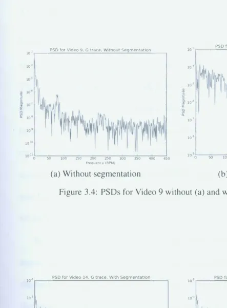
The power spectral densities (Figures 3.4 and 3.5) provide a little more

information about may have occurred. In the PSDs without segmentation,

the true pulse - marked with a small circle - rises at least half an order of

magnitude above its surroundings in video 9, but barely rises above its sur­

roundings in video 14. In both cases, segmentation causes the spectrum to

flatten somewhat, making the peaks no longer as noticeable. In video 9, this

produces a false peak around 50 BPM; the peak at the true heart rate is still

present, but several more peaks have been introduced by the segmentation

process. Video 14 also presents spurious peaks, however those which would

mask the true heart rate are outside of the range used for maximum finding.

This flattening appears to be the source of the degradation that the chosen

segmentation method has introduced. The flattening could be a result of the

somewhat random nature of the segmentations: between frames, the number

of chosen pixels could vary by up to 10,000, and which artifacts from the

-

·-...

(a) Segmentation reduced accuracy (Video 9) (b) Segmentation did not harm (Video 14)

Figure 3.3: Sample frames from two videos in which segmentation hurt results (a) and in which it did not (b)

modulate the traces and could be spreading out some of the spectral content.

Finally, it is worth noting that the addition of segmentation

preprocess-ing was a net improvement for the cICA estimates. As with the PSD-based methods, segmentation improved some videos and degraded others, but,

overall, it improved more than it harmed: 23 out of the tested 40 videos

were within 5% of the correct value using plain cICA; when segmentation was added, this number increased to 25 videos. This might suggest that

background content reduced the cICA methods' accuracy; the

segmenta-tion could have reduced this anomalous content. If this is true, then the background content is not the most significant limiter for the other pulse

10 � PSD tor Video 9. G trace, Without Segmentation

10'

10� 109

10 10

10� � -

= -

=

(a) Without segmentation

10 PSD for Video 9. G trace, With Segmentation

10'

101\

10·6

10 1

10'

1M

10� m

= =

= =

= = - =

(b) With segmentation Figure 3.4: PSDs for Video 9 without (a) and with (b) segmentation

10., PSD for Video 14, G trace, With Segmentation

10·'

10 1

� m

= =

= = = = -

=

(a) Without segmentation

10, PSD for Video 14. G trace, With Segmentation

10

10'

�I

10'

10'

10\ m

= =

= =

=

= -

=

3.2.2 ALE

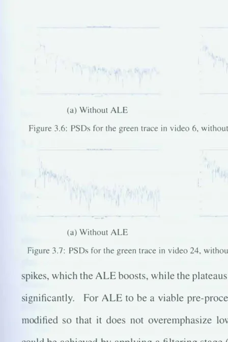
Similarly, adaptive line enhancement ( column E) causes some estimates -such as those for video 6- to improve and others - as in video 8 - to worsen. This could indicate that the adaptive line enhancer is enhancing the wrong frequencies, since the waveforms contain non-negligible low frequency con­ tent. Further evidence for this possibility comes from the relatively low estimates after ALE processing: in the worst case (the B channel), only I estimate (2.5%) was more than 60 BPM, compared to 35 (87 .5%) of the ac­ tual heart rates; even in the best case (a*), only 16 estimates ( 40%) exceeded 60 BPM.

(a) Without ALE (b) With ALE

Figure 3.6: PSDs for the green trace in video 6, without (a) and with (b) ALE applied

(a) Without ALE (b) With ALE

Figure 3.7: PSDs for the green trace in video 24, without (a) and with (b) ALE applied

(as implemented, this is the mean-squared error) could be modified to favor "reasonable" frequencies. This approach could require more effort, because its effects on the output are less direct than filtering. However, this method may also produce more reliable results, since rejecting inappropriate content becomes part of the ALE's operation.

3.2.3 Homomorphic Filtering

Homomorphic filtering does not seem to produce any significant changes to the estimate. This is likely due to a lack of additional filtering in the new (logarithmic) domain to reduce noise. Without further filtering, the loga­ rithm only serves to change the scaling of the data by attenuating large sam­ ples without greatly impacting smaller ones. The resulting spectra greatly resemble the original spectra, apart from a reduction in amplitude due to the reduction in the data's scale.

is not present. Instead, a bandpass filter with multiple passbands would be needed so that this spread out content is not lost. These additional bands would require greater design effort: they need to be placed to capture the signal content, narrow enough to reject the noise, and their relative attenua­ tions would need to be adjusted if a sinusoidal output is desired.

3.2.4 Alternative Color Spaces

The color space in which the processing is performed has a much stronger impact on estimate reliability. The a* channel of the L *a*b* color space produced 23 estimates (out of 40 trials) that were within 5% of the cor­ rect value, while the B channel of RGB space only produced 4 good esti­ mates. The a* results are comparable to the results for the cICA methods (Table C.17), but run in significantly less time. After a*, the next best chan­ nels were u (Luv) and Cr (YCrCb) with 16 good estimates each, followed by G (RGB), Y and Cb (YCrCb), and b* (L*a*b*) with 13 good estimates. The best performing channels (a*, u, and Cr) are chrominance channels which measure the red to green content of the color, followed by the other chrominance and luminance channels and the original green channel.

be detecting greater changes than the original RGB channels since chromi­ nance could be viewed as a measure of color difference. Consequently, the chrominance channel may be rejecting some noise common to the RGB channels. The effectiveness of the G channel was originally noted in [14], where it was suggested that this was due to hemoglobin's high absorption of green light. The luminance channels may be producing similar perfor­ mance to the G channel because perceived luminance correlates well with green content.

3.3 Video Performance

Another way to analyze the results is to observe that some videos - espe­ cially Videos 7, 10, and 40 - produced good heart rate estimates across several color spaces and processing methods, while others - notably 18, 19, and 20 - did not yield reasonable estimates under any applied method­ ology. This suggests that there may be some characteristics of the video which can significantly impact the ability to extract a heart rate estimate. Subject motion is an obvious factor; however, there was no significant sub­ ject movement in most of the videos since they were taken in a controlled

moved. The degree to which the face filled the frame was another notice­ able difference between the videos whose predictions were more reliable (the person's face filled almost the entire frame) or less reliable (more than half of the frame consisted of non-face pixels).

3.4 PPG Extraction

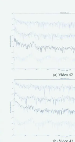
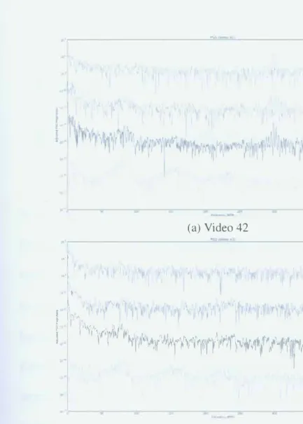
Figure 3.8 shows the power spectral densities (PSDs) for the extracted red, green, and blue channels in comparison to the PSD for a PPG recording taken during video recording in the absence of additional pre- and post­ processing techniques. In all three cases, the green channel exhibits a peak at the same fundamental frequency as the PPG, which is also visible in the red and blue channels in videos 42 and 43. The agreement is not perfect, however. All of the traces exhibit significant low frequency content that is not present in the PPG signal. This poses a problem for extracting respi­ ratory information from the signals, since this spurious content masks the lower frequency parts of the PPG signal from which respiratory character­ istics are extracted. Additionally, videos 42 and 44 exhibit artifacts around

"f

·I

! "

} r�·�

;11\\h l,.. I _{I 1}

I

t ·[

l"C.OIVldMl•l!

(a) Video 42

,a,K,OO<P"c<"'m� �,1,-,•�l"J)f"hun,G [Xlr�, tl'd >l>l!<t•ur,1 B PP<;S1M<tn,,,..

, ·

,..,�

..,

,.-9

.

,

l ', _{,, '}

.

'

i1

1 \\ r Tl

' ' Tr

n

t ...

I

�,, I

(b) Video 43

(c) Video 44

E•1r...:•tod"'fH'<trumR lx!le<'l!"li"f)f'·-lrun,C. htr•�tNs�t·ufT·B Pf'GSpe,ctrum

r:f-'/J �i:,.�if _{i, ,1}

r,i;;r

P<;OtVl<M'o•n

l

·_,1 ,. 11�

I

I��.,

I ,II �',.f,• ' I ,, ... -. • -. (, 11 n1l_{1'11J, I\}

f ,f

f

t"it'"

:1N1

,. I' . I _�\,•

(a) Video 42

(b) Video 43 ...-.01�•·11

1•1! _{� lt-J, '"} v n, · ,tr _{',t,'11r\ 1\t1i}f_{•11 ''}

!'If I 1, 111 ,

I'

(c) Video 44

frtr•rtH�trco,...,L.'I f>tf•Utf'<l...,...:trur-,1• ht•¥.ted�p,t<.trur b• l"PGSpe,ctn,m

,,.I ··1

l •

(a) Video 42

h,,.,tPl'l\�'l'Y t,,, ... c1"(-ll\l1T' Ea1r•t"<i14>1"Ctlun b PPG S9ttt•1,1r1

ht .. ,tNl,l"'("tnJfT"Y I

�::::�::: ::::����I PPG<;i>.<tn,m

...,

I' i I •1'"

. , I ;\,,.,, •·, v,

•. 11,111 � � _{1111,1, .,., W}1 _,I

I . ! .,,. -4.t,i. _{'t'1l11/1,/ .,� ••} ..,,.l l•"'fij/1 ,11

l '

'i'' ' �1\1",,f "/

r1t11'1"1f

rrir1

I.,.,

'f �

I

I

"'

l;

, lr '��·

r

(b) Video 43

I,

(c) Video 44

fJfr•<tM,i--tn.rrY h!r••tPd�,...uw,,c., ic .. turcl��pe,..trun lbj PPGSpe,ct,um

I ·11:_.i,,,,·1,1"'_{�1'['1� ,1i1,1}

\·,,.·;\�'1t'1 f '1_{1i I 11}

111, I

Chapter 4

Future Research Directions

There are many ways in which this research could potentially be extended. For example, the current homomorphic filtering step simply takes a loga­ rithm to transform the signal and noise components from a multiplicative to a linear combination according to the model (2.4 ).A more sophisticated homomorphic filter would apply a carefully constructed low- or band-pass filter to suppress this noise component more. The design of such a filter would require care, however, since the logarithm will tend to spread spec­ tral lines into their harmonics, too.

but there are some characteristics of the PPG waveform that could be cap­ tured by the ALE, such as the suppression of content with very ]ow frequen­ cies: when the ALE was applied to the observed traces, the output tended to emphasize the low frequency content (much below the heart rate), to the detriment of the heart rate estimation. Another simple feature of the PPG spectrum that the ALE could incorporate is the presence of harmonics. In the PPG spectrum (see, for example, Figure 3.8), the fundamental and first three harmonics are clearly visible. This information could be used to better reject noise, since any spurious peaks in a noisy signal should not possess significant harmonic content.

It is also possible that an IIR model may have been more suitable for the ALE. While a linear combiner (FIR filter) model was chosen for its sim­ plicity and stability, the potential instability of an IIR filter could potentially improve the extracted spectra, since the presence of pure sinusoids would require poles at their frequencies.

similar in color and sufficiently close to the person) and should thus also remain the same size over time. This would also be more practical in a less controlled setting, where face tracking would need to be applied to deter­ mine the location of the face before processing. In fact, the face tracking algorithm could be designed to output the average taken over only the face pixels, rather than a rectangular region requiring further processing. This would be more efficient and likely more stable than the color-based seg­ mentation approach used here.

Chapter 5

Conclusions

Comparison of the tabulated heart rate estimates suggests that the a* chan­ nel provides a good predictor of heart rate. It performed comparably to the cICA algorithm, but with a much shorter run time. More generally, the chrominance-based channels performed better than their luminance-based counterparts. This may be because the chrominance channels should be more robust to non-uniform lighting- a source of error which is ideally cap­ tured in its entirety by the luminance channel, or it is possible that chromi­ nance spaces suppress noise common to the R, G, and B channels, since chrominance represents a "difference" in color.

Bibliography

[1] USB device class definition for video devices, 2012.

[2] John Allen. Photoplethysmography and its applications in clinical physilogical measurement. Physiological Measurement, 28:Rl-R39, January 2007.

[3] Arne Broman. Introduction to Partial Differential Equations: From Fourier Series to Boundary-Value Problems, pages 23-25. Addison­ Wesley Pub. Co., Reading, Mass., 1970.

[ 4] Gerard de Haan and Vincent Jeanne. Robust pulse rate from chrominance-based rppg. IEEE Transaction on Biomedical Engineer­ ing, 60:2878-2886, October 2013.

[5] M. Ghogho, M. Ibnkahla, and N.J. Bershad. Analytic behavior of the lms adaptive line enhancer for sinusoids corrupted by multiplicative and additive noise. IEEE Transactions on Signal Processing, 46:2386-2393, September 1998.

[6] Rafael C. Gonzalez and Richard E. Woods. Digital Image Processing, Third Edition, pages 394-456. Pearson Prentice Hall, Upper Saddle River, New Jersey, 2008.

[8] Keith Jack. Video Demystified: A Handbook for the Digital Engineer (5th Edition), pages 15-763. Newnes, Burlington, Mass., 2007.

[9] Alan V. Oppenheim, Alan S. Willsky, and S. Hamid Nawab. Signals & Systems, Second Edition, pages 314-321. Prentice Hall, Upper Saddle River, New Jersey, 1997.

[10] I. Pitas and A.N. Venetsanapoulos. Nonlinear Digital Filters: Princi­ ples and Applications, pages 217-244. Kluwer Academic Publishers, Boston, 1990.

[11] Ming-Zher Poh, Daniel J. McDuff, and Rosalind W. Picard. Non­ contact, automated cardiac pulse measurements using video imaging and blind source separation. Optics Express, 18:10762-10774, May 2010.

[12] Ming-Zher Poh, Daniel J. McDuff, and Rosalind W. Picard. Advance­ ments in noncontact, multiparameter physiological measurements us­ ing a webcam. IEEE Transactions on Biomedical Engineering, 58:7-11, January 2011.

[13] Gill R. Tsouri, Survi Kyal, Sohail Dianat, and Lalit K. Mestha. Con­ strained independent component analysis approach to nonobtrusive pulse rate measurements. Journal of Biomedical Optics, 17: 077011-1-077011-4, July 2012.

[14] Wim Verkruysse, Lars O Svaasand, and J Stuart Nelson. Remote plethysmographic imaging using ambient light. Optics Express, 26:21434-21445, December 2008.

[16] Stephen Ripamonti Westland and Vien Caterina Cheung. Computa­ tional Colour Science using MATLAB, pages 48-74. Wiley, Somerset, New Jersey, 2012.

Appendix A

Segmentation Algorithm

##################################################

# segmentationMethod #

################################################## # Opens a video and produces a set of RGB traces # # by applying a naive segmentation method each #

# frame. #

##################################################

# Args: #

# filename Name of the video #

# trans Transform #

##################################################

# Outputs: #

# y s RGB t r a c e v a l u e s #

##################################################

def segmentationMethod (filename, trans, preprocessTrans = None): # Set up some useful variables

vid = cv2. VideoCapture( filename)

vi d Len = i n t ( v i d . get ( c v 2 . c v . CV _CAP _pRQP _FRAME_COUNT) ) ys = np.zeros((2* vidLen, 3))

bins = np.array(xrange(O, 256)) = 0

# Find inverse transform

invTrans = invTransTable [ trans]

# Convert color space

ret , frame = vid. read()

maxY, maxX = frame. shape[: - I]

area = float(frame.shape[O] * frame.shape[!]) frame = cv2.cvtColor(frame, trans )

frame = np.transpose(frame, ( 2,1,0))

# Iterate over frames

while re t:

for c in xrange (0, 2):

hist = cv2.calcHist(frame, [c], None, [256], [O, 256]) I area

prob = 0.3 # Save peak

peak = hist. argmax () accProb = hist [peak] incrMax = I

incrMin = I

# Accumulate pixels until (prob)% of the pixels have been amassed

while accProb < prob:

if peak - incrMin < 0 or ( peak + incrMax < 230 and hist[peak + incrMax] > hist[peak - incrMin ]):

incrMax += I

a c c Pro b += h i s t [ peak + i n c r Max ] else

incrMin +=

accProb += hist[peak-incrMin] # Threshold frame

condition = np.logicaLor(frame[c,:,:] > peak + incrMax, frame[c,: ,:] < peak - incrMin)

frame = np. transpose (frame, ( 2, l ,0))

frame = cv2.cvtColor(frame, invTrans)

if preprocessTrans is not None:

frame = cv2. cvtColor (frame, p reprocessTrans)

ys [ i , O] ys [ i , I] ys[i, 2)

frame[condition .T, OJ.mean() frame[condition.T, !].mean() = frame[condition .T, 2].mean()

# Next iteration

rel, frame = vid. read() if not ret:

break

# Transpose needed for histogram; crop to face and apply color space transformation

frame = cv2.cvtColor(frame, trans) frame = np.transpose(frame, ( 2,1,0))

i+=l vid. release()

Appendix B

Adaptive Line Enhancer Algorithm

#################################################

# applyALE #

################################################# # Applies adaptive line enhancer to trace # #################################################

# Args: #

# y s Old RGB tr a c e val u es # #################################################

# Outputs: #

# ys New RGB trace values # #################################################

def applyALE(ys):

# Filter parameters order = 512 de I ta = 20

mu 9e-4

# Model/ signal parameters # Sampling frequency

fs = 15.0

# Length of W

# Delay to decorrelate # Learning rate

window = sig. boxc ar ( order)

# Initialize weights, signal,

length = len(ys)

# LMS algorithm

and noises

# Sample length

w = np. zeros ( ( I , order) , d type=np. complex 128)

# Set the desired signal to be zero mean to improve convergence z = ys. reshape(len(ys))

z = z - z . mean () z. reshape (( len (z)))

# LMS algorithm

eps = np.zeros_like(z) res = np. zeros_like(z) dw = np.zeros_like(z)

m i n I n de x = max ( 0 , k -d e I t a -o r d e r + I ) m ax I n de x = max ( 0 , k -d e I t a + I )

shape = maxlndex-minlndex

if shape > 0:

samples [O: shape ] =

z [ min lndex: maxlndex] [:: -I]. reshape ((shape, I)) y = w.dot(samples )

res[k:(k+I)] = y

eps[k:(k+I)] = (z[k:(k+I)] - y) I (I + n p . sum ( n p . abs ( s amp I es ) ** 2) )

dw[k:(k+l )] = np. sqrt(np.sum(np.abs(mu * eps[k] * samples. conjugate (). T) **2))

w += mu * e p s [ k : ( k + I ) ] * s amp I es . conj u gale () . T

Appendix C

Tables of Results

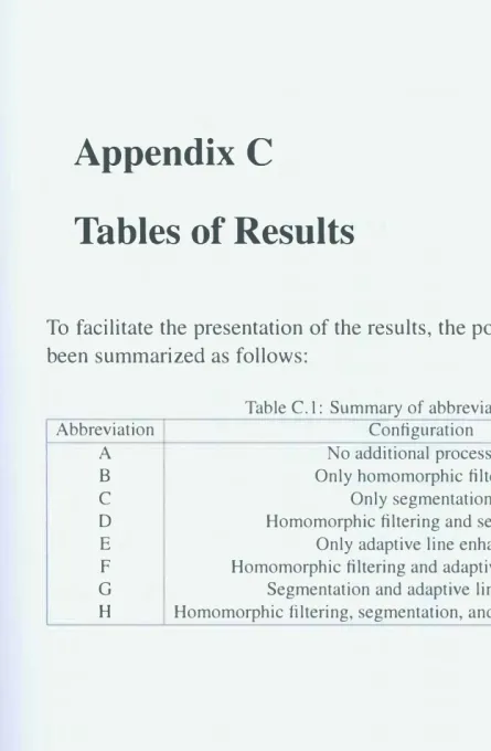
To facilitate the presentation of the results, the possible configurations have been summarized as follows:

Table C.1: Summary of abbreviations

Abbreviation Configuration

A No additional processing

B Only homomorphic filtering

C Only segmentation

D Homomorphic filtering and segmentation

E Only adaptive line enhancer

F Homomorphic filtering and adaptive line enhancer G Segmentation and adaptive line enhancer

Video 1 2 3 4 5 6 7 8 9 10 11 12 13 14 15 16 17 18 19 20 21 22 23 24 25 26 27 28 29 30

Table C.2: Heart rate estimates - red channel (RGB)

Actual A B C D E F G

84 75.0 75.0 47.1 47.1 42.7 42.7 41.0 53 46.1 46.1 52.4 52.4 46.1 46.1 44.0 63 46.7 46.7 44.9 44.9 42.2 42.2 44.9

82 79.1 79.1 48.1 48.1 43.0 43.0 43.8 83 42.7 42.7 49.9 49.9 41.9 41.9 74.1 64 50.5 50.5 44.8 44.8 57.1 57.1 79.0

61 63.8 63.8 64.9 64.9 61.8 61.8 65.9 72 40.7 40.7 71.9 71.9 40.7 40.7 40.7

78 54.0 54.0 41.0 41.0 54.0 54.0 41.0 94 49.6 49.6 109.5 109.5 49.6 49.6 53.7 53 42.8 42.8 41.8 41.8 42.8 42.8 42.8

66 43.4 43.4 70.2 70.2 48.9 48.9 69.2 63 43.1 43.1 50.9 50.9 43.1 43.1 50.9 60 52.7 52.7 68.7 68.7 52.7 52.7 68.7 68 41.4 41.4 48.3 48.3 42.4 42.4 48.3 78 45.8 45.8 60.4 60.4 45.8 45.8 43.8 57 41.3 41.3 42.2 42.2 40.4 40.4 43.1 73 60.7 60.7 58.0 58.0 42.8 42.8 58.0 68 40.0 40.0 55.1 55.1 40.0 40.0 55.1 66 44.0 44.0 41.0 41.0 40.0 40.0 41.0 76 42.0 42.0 111.1 111.1 42.0 42.0 112.1 68 68.1 68.1 58.1 58.1 52.1 52.1 42.0 66 45.1 45.1 44.0 44.0 55.1 55.1 44.0

100 40.0 40.0 44.0 44.0 44.0 44.0 44.0 113 40.0 40.0 40.0 40.0 45.1 45.1 44.0 63 216.2 216.2 122.1 122.1 56.1 56.1 74.1 60 40.0 40.0 82.1 82.1 41.0 40.0 45.1 67 170.2 170.2 138.2 138.2 65.1 65.1 75.1 76 92.1 92.1 50.1 50.1 50.1 50.1 50.1 97 96.1 96.1 41.0 41.0 47.1 47.1 63.1

Video 1 2 3 4 5 6 7 8 9 10 11 12 13 14 15 16 17 18 19 20 21 22 23 24 25 26 27 28 29 30

Table C.3: Heart rate estimates - green channel (RGB)

Actual A B C D E F G

84 75.0 75.0 47.1 47.1 42.7 42.7 41.0 53 46.1 46.1 52.4 52.4 46.1 46.1 44.0 63 46.7 46.7 44.9 44.9 42.2 42.2 44.9 82 79.1 79.1 48.1 48.1 43.0 43.0 43.8 83 42.7 42.7 49.9 49.9 41.9 41.9 74.1 64 50.5 50.5 44.8 44.8 57.1 57.1 79.0 61 63.8 63.8 64.9 64.9 61.8 61.8 65.9 72 40.7 40.7 71.9 71.9 40.7 40.7 40.7 78 54.0 54.0 41.0 41.0 54.0 54.0 41.0 94 49.6 49.6 109.5 109.5 49.6 49.6 53.7 53 42.8 42.8 41.8 41.8 42.8 42.8 42.8 66 43.4 43.4 70.2 70.2 48.9 48.9 69.2 63 43.1 43.1 50.9 50.9 43.1 43.1 50.9 60 52.7 52.7 68.7 68.7 52.7 52.7 68.7 68 41.4 41.4 48.3 48.3 42.4 42.4 48.3 78 45.8 45.8 60.4 60.4 45.8 45.8 43.8 57 41.3 41.3 42.2 42.2 40.4 40.4 43.1 73 60.7 60.7 58.0 58.0 42.8 42.8 58.0 68 40.0 40.0 55.1 55.1 40.0 40.0 55.1 66 44.0 44.0 41.0 41.0 40.0 40.0 41.0 76 42.0 42.0 111.1 111.1 42.0 42.0 112.1 68 68.1 68.1 58.1 58.1 52.1 52.1 42.0

66 45.1 45.1 44.0 44.0 55.1 55.1 44.0 100 40.0 40.0 44.0 44.0 44.0 44.0 44.0 113 40.0 40.0 40.0 40.0 45.1 45.1 44.0 63 216.2 216.2 122.1 122.1 56.1 56.1 74.1 60 40.0 40.0 82.1 82.1 41.0 40.0 45.1 67 170.2 170.2 138.2 138.2 65.1 65.1 75.1 76 92.1 92.1 50.1 50.1 50.1 50.1 50.1 97 96.1 96.1 41.0 41.0 47.1 47.1 63.1

31 62 40.0 40.0 49.1 49.1 41.0 41.0 42.0 42.0 32 70 40.0 40.0 78.1 78.1 43.0 43.0 44.0 44.0

33 86 43.0 43.0 72.1 72.1 44.0 44.0 47.1 48.1 34 57 75.1 75.1 228.3 228.3 40.0 40.0 41.0 41.0 35 72 42.0 42.0 106.1 106.1 42.0 42.0 106.1 106.1

36 96 42.0 42.0 42.0 42.0 41.0 41.0 41.0 41.0

37 69 40.0 40.0 40.0 41.0 40.0 40.0 42.0 42.0

38 64 48.1 48.1 72.1 72.1 48.1 48.1 46.1 46.1 39 74 55.1 55.1 55.1 55.1 56.1 56.1 40.0 56.1 40 60 60.1 60.1 61.1 61.1 40.0 40.0 40.0 40.0

41 49 56.1 56.1 55.1 55.1 56.1 56.1 50.1 50.1

42 79 86.8 86.8 52.2 52.2 86.8 86.8 52.2 52.2 43 75 65.0 65.0 62.7 62.7 55.7 55.7 62.2 62.2

Video 1 2 3 4 5 6 7 8 9 10 11 12 13 14 15 16 17 18 19 20 21 22 23 24 25 26 27 28 29 30

Table C.4: Heart rate estimates - blue channel (RGB)

Actual A B C D E F G

84 75.0 75.0 47.1 47.1 42.7 42.7 41.0

53 46.1 46.1 52.4 52.4 46.1 46.1 44.0

63 46.7 46.7 44.9 44.9 42.2 42.2 44.9 82 79.1 79.1 48.1 48.1 43.0 43.0 43.8 83 42.7 42.7 49.9 49.9 41.9 41.9 74.1 64 50.5 50.5 44.8 44.8 57.1 57.1 79.0 61 63.8 63.8 64.9 64.9 61.8 61.8 65.9 72 40.7 40.7 71.9 71.9 40.7 40.7 40.7 78 54.0 54.0 41.0 41.0 54.0 54.0 41.0 94 49.6 49.6 109.5 109.5 49.6 49.6 53.7 53 42.8 42.8 41.8 41.8 42.8 42.8 42.8 66 43.4 43.4 70.2 70.2 48.9 48.9 69.2 63 43.1 43.1 50.9 50.9 43.1 43.1 50.9 60 52.7 52.7 68.7 68.7 52.7 52.7 68.7

68 41.4 41.4 48.3 48.3 42.4 42.4 48.3 78 45.8 45.8 60.4 60.4 45.8 45.8 43.8 57 41.3 41.3 42.2 42.2 40.4 40.4 43.1 73 60.7 60.7 58.0 58.0 42.8 42.8 58.0

68 40.0 40.0 55.1 55.1 40.0 40.0 55.1

66 44.0 44.0 41.0 41.0 40.0 40.0 41.0 76 42.0 42.0 111.1 111.1 42.0 42.0 112.1 68 68.1 68.1 58.1 58.1 52.1 52.1 42.0 66 45.1 45.1 44.0 44.0 55.1 55.1 44.0

100 40.0 40.0 44.0 44.0 44.0 44.0 44.0

113 40.0 40.0 40.0 40.0 45.1 45.1 44.0 63 216.2 216.2 122.1 122.1 56.1 56.1 74.1 60 40.0 40.0 82.1 82.1 41.0 40.0 45.1

67 170.2 170.2 138.2 138.2 65.l 65.1 75.1 76 92.1 92.1 50.1 50.1 50.1 50.1 50.1 97 96.1 96.1 41.0 41.0 47.1 47.1 63.1

31 62 40.0 40.0 49.1 49.1 41.0 41.0 42.0 42.0 32 70 40.0 40.0 78.1 78.1 43.0 43.0 44.0 44.0 33 86 43.0 43.0 72.1 72.1 44.0 44.0 47.1 48.1 34 57 75.1 75.1 228.3 228.3 40.0 40.0 41.0 41.0 35 72 42.0 42.0 106.1 106.1 42.0 42.0 106.1 106.1 36 96 42.0 42.0 42.0 42.0 41.0 41.0 41.0 41.0 37 69 40.0 40.0 40.0 41.0 40.0 40.0 42.0 42.0 38 64 48.1 48.1 72.1 72.1 48.1 48.1 46.1 46.1 39 74 55.1 55.1 55.1 55.1 56.1 56.1 40.0 56.1 40 60 60.1 60.1 61.1 61.1 40.0 40.0 40.0 40.0

41 49 56.1 56.1 55.1 55.1 56.1 56.1 50.1 50.1

Video l 2 3 4 5 6 7 8 9 10 11 12 13 14 15 16 17 18 19 20 21 22 23 24 25 26 27 28 29 30

Table C.5: Heart rate estimates - hue channel (HSY)

Actual A B C D E F G

84 75.0 75.0 47.1 47.1 42.7 42.7 41.0 53 46.1 46.1 52.4 52.4 46.1 46.1 44.0

63 46.7 46.7 44.9 44.9 42.2 42.2 44.9

82 79.l 79.1 48.1 48.1 43.0 43.0 43.8 83 42.7 42.7 49.9 49.9 41.9 41.9 74.1 64 ·50.5 50.5 44.8 44.8 57.1 57.1 79.0

61 63.8 63.8 64.9 64.9 61.8 61.8 65.9

72 40.7 40.7 71.9 71.9 40.7 40.7 40.7 78 54.0 54.0 41.0 41.0 54.0 54.0 41.0

94 49.6 49.6 109.5 109.5 49.6 49.6 53.7 53 42.8 42.8 41.8 41.8 42.8 42.8 42.8 66 43.4 43.4 70.2 70.2 48.9 48.9 69.2 63 43.1 43.1 50.9 50.9 43.1 43.1 50.9 60 52.7 52.7 68.7 68.7 52.7 52.7 68.7 68 41.4 41.4 48.3 48.3 42.4 42.4 48.3 78 45.8 45.8 60.4 60.4 45.8 45.8 43.8

57 41.3 41.3 42.2 42.2 40.4 40.4 43.1

73 60.7 60.7 58.0 58.0 42.8 42.8 58.0 68 40.0 40.0 55.1 55.1 40.0 40.0 55.1 66 44.0 44.0 41.0 41.0 40.0 40.0 41.0 76 42.0 42.0 111.1 111.1 42.0 42.0 112.1 68 68.1 68.1 58.1 58.1 52.1 52.1 42.0 66 45.1 45.1 44.0 44.0 55.1 55.1 44.0 100 40.0 40.0 44.0 44.0 44.0 44.0 44.0 113 40.0 40.0 40.0 40.0 45.1 45.1 44.0

63 216.2 216.2 122.1 122.1 56.1 56.1 74.1

60 40.0 40.0 82.1 82.1 41.0 40.0 45.1

67 170.2 170.2 138.2 138.2 65.1 65.l 75.1

76 92.1 92.1 50.1 50.1 50.1 50.1 50.1

97 96.1 96.1 41.0 41.0 47.1 47.1 63.1

31 62 40.0 40.0 49.1 49.1 41.0 41.0 42.0 42.0 32 70 40.0 40.0 78.1 78.1 43.0 43.0 44.0 44.0 33 86 43.0 43.0 72.1 72.1 44.0 44.0 47.1 48.1 34 57 75.1 75.1 228.3 228.3 40.0 40.0 41.0 41.0

35 72 42.0 42.0 106.1 106.1 42.0 42.0 106.1 106.1

36 96 42.0 42.0 42.0 42.0 41.0 41.0 41.0 41.0

37 69 40.0 40.0 40.0 41.0 40.0 40.0 42.0 42.0

Video 1 2 3 4 5 6 7 8 9 10 11 12 13 14 15 16 17 18 19 20 21 22 23 24 25 26 27 28 29 30

Table C.6: Heart rate estimates - saturation chan­ nel (HSV)

Actual A B C D E F G

84 75.0 75.0 47.1 47.1 42.7 42.7 41.0 53 46.1 46.1 52.4 52.4 46.1 46.1 44.0 63 46.7 46.7 44.9 44.9 42.2 42.2 44.9 82 79.1 79.1 48.1 48.1 43.0 43.0 43.8 83 42.7 42.7 49.9 49.9 41.9 41.9 74.1 64 50.5 50.5 44.8 44.8 57.1 57.1 79.0 61 63.8 63.8 64.9 64.9 61.8 61.8 65.9 72 40.7 40.7 71.9 71.9 40.7 40.7 40.7

78 54.0 54.0 41.0 41.0 54.0 54.0 41.0 94 49.6 49.6 109.5 109.5 49.6 49.6 53.7 53 42.8 42.8 41.8 41.8 42.8 42.8 42.8 66 43.4 43.4 70.2 70.2 48.9 48.9 69.2 63 43.1 43.1 50.9 50.9 43.1 43.1 50.9 60 52.7 52.7 68.7 68.7 52.7 52.7 68.7 68 41.4 41.4 48.3 48.3 42.4 42.4 48.3 78 45.8 45.8 60.4 60.4 45.8 45.8 43.8 57 41.3 41.3 42.2 42.2 40.4 40.4 43.1 73 60.7 60.7 58.0 58.0 42.8 42.8 58.0 68 40.0 40.0 55.1 55.1 40.0 40.0 55.1 66 44.0 44.0 41.0 41.0 40.0 40.0 41.0 76 42.0 42.0 111.1 111.1 42.0 42.0 112.1 68 68.1 68.1 58.1 58.1 52.1 52.1 42.0 66 45.1 45.1 44.0 44.0 55.1 55.1 44.0 100 40.0 40.0 44.0 44.0 44.0 44.0 44.0 113 40.0 40.0 40.0 40.0 45.1 45.1 44.0 63 216.2 216.2 122.1 122.1 56.1 56.1 74.1 60 40.0 40.0 82.1 82.1 41.0 40.0 45.1 67 170.2 170.2 138.2 138.2 65.1 65.1 75.1 76 92.1 92.1 50.1 50.1 50.1 50.1 50.1 97 96.1 96.1 41.0 41.0 47.1 47.1 63.1

Video 1 2 3 4 5 6 7 8 9 10 11 12 13 14 15 16 17 18 19 20 21 22 23 24 25 26 27 28 29 30

Table C.7: Heart rate estimates - value channel (HSV)

Actual A B C D E F G

84 75.0 75.0 47.1 47.1 42.7 42.7 41.0 53 46.1 46.1 52.4 52.4 46.1 46.1 44.0 63 46.7 46.7 44.9 44.9 42.2 42.2 44.9 82 79.1 79.1 48.1 48.1 43.0 43.0 43.8 83 42.7 42.7 49.9 49.9 41.9 41.9 74.l 64 50.5 50.5 44.8 44.8 57.1 57.1 79.0 61 63.8 63.8 64.9 64.9 61.8 61.8 65.9 72 40.7 40.7 71.9 71.9 40.7 40.7 40.7 78 54.0 54.0 41.0 41.0 54.0 54.0 41.0 94 49.6 49.6 109.5 109.5 49.6 49.6 53.7 53 42.8 42.8 41.8 41.8 42.8 42.8 42.8 66 43.4 43.4 70.2 70.2 48.9 48.9 69.2 63 43.1 43.1 50.9 50.9 43.1 43.l 50.9 60 52.7 52.7 68.7 68.7 52.7 52.7 68.7 68 41.4 41.4 48.3 48.3 42.4 42.4 48.3 78 45.8 45.8 60.4 60.4 45.8 45.8 43.8 57 41.3 41.3 42.2 42.2 40.4 40.4 43.1 73 60.7 60.7 58.0 58.0 42.8 42.8 58.0 68 40.0 40.0 55.1 55.1 40.0 40.0 55.1 66 44.0 44.0 41.0 41.0 40.0 40.0 41.0 76 42.0 42.0 111.1 111.1 42.0 42.0 112.1 68 68.1 68.1 58.1 58.1 52.1 52.1 42.0 66 45.l 45.1 44.0 44.0 55.1 55.1 44.0 100 40.0 40.0 44.0 44.0 44.0 44.0 44.0 113 40.0 40.0 40.0 40.0 45.1 45.1 44.0 63 216.2 216.2 122.1 122.1 56.1 56.1 74.1 60 40.0 40.0 82.1 82.1 41.0 40.0 45.1 67 170.2 170.2 138.2 138.2 65.1 65.1 75.1 76 92.1 92.1 50.1 50.1 50.1 50.1 50.1 97 96.1 96.1 41.0 41.0 47.1 47.1 63.1

Table C.8: Heart rate estimates - L channel (Luv)

Video Actual A B C D E F G H

Table C.9: Heart rate estimates - u channel (Luv)

Video Actual A B C D E F G H

Table C.10: Heart rate estimates- v channel (Luv)

Video Actual A B C D E F G H

1 84 75.0 75.0 47.1 47.1 42.7 42.7 41.0 41.0 2 53 46.1 46.1 52.4 52.4 46.1 46.1 44.0 67.1

3 63 46.7 46.7 44.9 44.9 42.2 42.2 44.9 44.9

4 82 79.1 79.1 48.1 48.1 43.0 43.0 43.8 43.8 5 83 42.7 42.7 49.9 49.9 41.9 41.9 74.1 74.1

6 64 50.5 50.5 44.8 44.8 57.1 57.1 79.0 79.0 7 61 63.8 63.8 64.9 64.9 61.8 61.8 65.9 65.9 8 72 40.7 40.7 71.9 71.9 40.7 40.7 40.7 40.7

9 78 54.0 54.0 41.0 41.0 54.0 54.0 41.0 41.0 10 94 49.6 49.6 109.5 109.5 49.6 49.6 53.7 53.7 11 53 42.8 42.8 41.8 41.8 42.8 42.8 42.8 42.8 12 66 43.4 43.4 70.2 70.2 48.9 48.9 69.2 69.2 13 63 43.1 43.1 50.9 50.9 43.1 43.1 50.9 50.9 14 60 52.7 52.7 68.7 68.7 52.7 52.7 68.7 68.7

15 68 41.4 41.4 48.3 48.3 42.4 42.4 48.3 48.3 16 78 45.8 45.8 60.4 60.4 45.8 45.8 43.8 43.8 17 57 41.3 41.3 42.2 42.2 40.4 40.4 43.1 43.1 18 73 60.7 60.7 58.0 58.0 42.8 42.8 58.0 57.1 19 68 40.0 40.0 55.1 55.1 40.0 40.0 55.1 55.1 20 66 44.0 44.0 41.0 41.0 40.0 40.0 41.0 41.0 21 76 42.0 42.0 111.1 111.1 42.0 42.0 112.1 112.1 22 68 68.1 68.1 58.1 58.1 52.1 52.1 42.0 42.0

23 66 45.1 45.1 44.0 44.0 55.1 55.1 44.0 44.0 24 100 40.0 40.0 44.0 44.0 44.0 44.0 44.0 44.0 25 113 40.0 40.0 40.0 40.0 45.1 45.1 44.0 44.0 26 63 216.2 216.2 122.1 122.1 56.1 56.1 74.1 75.1 27 60 40.0 40.0 82.1 82.1 41.0 40.0 45.1 45.1

28 67 170.2 170.2 138.2 138.2 65.1 65.1 75.1 75.1

32 70 40.0 40.0 78.1 78.1 43.0 43.0 44.0 44.0

Video 1 2 3 4 5 6 7 8 9 10 11 12 13 14 15 16 17 18 19 20 21 22 23 .24·

25 26 27 28 29 30

Table C.11: Heart rate estimates - Y channel (YCbCr)

Actual A B C D E F G

84 75.0 75.0 47.1 47.1 42.7 42.7 41.0 53 46.1 46.1 52.4 52.4 46.1 46.1 44.0 63 46.7 46.7 44.9 44.9 42.2 42.2 44.9 82 79.1 79.1 48.1 48.1 43.0 43.0 43.8 83 42.7 42.7 49.9 49.9 41.9 41.9 74.1 64 50.5 50.5 44.8 44.8 57.1 57.1 79.0 61 63.8 63.8 64.9 64.9 61.8 61.8 65.9 72 40.7 40.7 71.9 71.9 40.7 40.7 40.7 78 54.0 54.0 41.0 41.0 54.0 54.0 41.0 94 49.6 49.6 109.5 109.5 49.6 49.6 53.7 53 42.8 42.8 41.8 41.8 42.8 42.8 42.8 66 43.4 43.4 70.2 70.2 48.9 48.9 69.2 63 43.1 43.1 50.9 50.9 43.1 43.1 50.9 60 52.7 52.7 68.7 68.7 52.7 52.7 68.7 68 41.4 41.4 48.3 48.3 42.4 42.4 48.3 78 45.8 45.8 60.4 60.4 45.8 45.8 43.8 57 41.3 41.3 42.2 42.2 40.4 40.4 43.1 73 60.7 60.7 58.0 58.0 42.8 42.8 58.0 68 40.0 40.0 55.1 55.1 40.0 40.0 55.1 66 44.0 44.0 41.0 41.0 40.0 40.0 41.0 76 42.0 42.0 111.1 111.1 42.0 42.0 112.1 68 68.1 68.1 58.1 58.1 52.1 52.1 42.0 66 45.1 45.1 44.0 44.0 55.1 55.1 44.0 100 40.0 40.0 44.0 44.0 44.0 44.0 44.0 113 40.0 40.0 40.0 40.0 45.1 45.1 44.0 63 216.2 216.2 122.1 122.1 56.1 56.1 74.1 60 40.0 40.0 82.1 82.1 41.0 40.0 45.1 67 170.2 170.2 138.2 138.2 65.1 65.1 75.1 76 92.1 92.1 50.1 50.1 50.1 50.1 50.1 97 96.1 96.1 41.0 41.0 47.1 47.1 63.1

31 62 40.0 40.0 49.1 49.1 41.0 41.0 42.0 42.0 32 70 40.0 40.0 78.1 78.1 43.0 43.0 44.0 44.0

33 86 43.0 43.0 72.1 72.1 44.0 44.0 47.1 48.1 34 57 75.1 75.1 228.3 228.3 40.0 40.0 41.0 41.0 35 72 42.0 42.0 106.1 106.1 42.0 42.0 106.1 106.1 36 96 42.0 42.0 42.0 42.0 41.0 41.0 41.0 41.0 37 69 40.0 40.0 40.0 41.0 40.0 40.0 42.0 42.0 38 64 48.1 48.1 72.1 72.l 48.1 48.1 46.1 46.1 39 74 55.1 55.1 55.1 55.1 56.1 56.1 40.0 56.1 40 60 60.1 60.1 61.1 61.1 40.0 40.0 40.0 40.0 41 49 56.1 56.1 55.1 55.1 56.1 56.1 50.1 50.1

42 79 86.8 86.8 52.2 52.2 86.8 86.8 52.2 52.2

Video 1