Chapter 5
EM
Geoffrey J. McLachlan and Shu-Kay Ng
Contents
5.1 Introduction . . . . 93
5.2 Algorithm Description . . . . 95
5.3 Software Implementation. . . . 96
5.4 Illustrative Examples . . . . 97
5.4.1 Example 5.1: Multivariate Normal Mixtures . . . . 97
5.4.2 Example 5.2: Mixtures of Factor Analyzers . . . .100
5.5 Advanced Topics. . . .103
5.6 Exercises . . . .105
References . . . .113
Abstract The expectation-maximization (EM) algorithm is a broadly applicable
approach to the iterative computation of maximum likelihood (ML) estimates, useful in a variety of incomplete-data problems. In particular, the EM algorithm simplifies considerably the problem of fitting finite mixture models by ML, where mixture models are used to model heterogeneity in cluster analysis and pattern recognition contexts. The EM algorithm has a number of appealing properties, including its numerical stability, simplicity of implementation, and reliable global convergence. There are also extensions of the EM algorithm to tackle complex problems in various data mining applications. It is, however, highly desirable if its simplicity and stability can be preserved.
5.1
Introduction
mixture models by maximum likelihood (ML) is a classic example of a problem that is simplified considerably by the EM’s conceptual unification of ML estimation from data that can be viewed as being incomplete [20]. Maximum likelihood estimation and likelihood-based inference are of central importance in statistical theory and data analysis. Maximum likelihood estimation is a general-purpose method with attractive properties [6, 13, 31]. Finite mixture distributions provide a flexible and mathematical-based approach to the modeling and clustering of data observed on random phenomena. We focus here on the use of the EM algorithm for the fitting of finite mixture models via the ML approach.
With the mixture model-based approach to clustering, the observed p-dimensional datay1, . . . ,yn are assumed to have come from a mixture of an initially specified number g of component densities in some unknown proportionsπ1, . . . , πg, which sum to 1. The mixture density ofyj is expressed as
f (yj;Ψ)= g
i=1
πifi(yj;i) ( j=1, . . . ,n) (5.1)
where the component density fi(yj;i) is specified up to a vectori of unknown parameters (i =1, . . . ,g). The vector of all the unknown parameters is given by
Ψ=π1, . . . , πg−1,T1, . . . ,Tg T
where the superscript T denotes vector transpose. The parameter vectorΨcan be
estimated by ML. The objective is to maximize the likelihood L(Ψ), or equivalently, the log likelihood log L(Ψ), as a function ofΨ, over the parameter space. That is, the ML estimate ofΨ, ˆΨ, is given by an appropriate root of the log likelihood equation,
∂log L(Ψ)/∂Ψ=0 (5.2)
where
log L(Ψ)= n
j=1
log f (yj;Ψ)
is the log likelihood function for Ψformed under the assumption of independent
datay1, . . . ,yn. The aim of ML estimation [13] is to determine an estimate ˆΨfor
5.2
Algorithm Description
The EM algorithm is an iterative algorithm, in each iteration of which there are two steps, the Expectation step (E-step) and the Maximization step (M-step). A brief history of the EM algorithm can be found in [18]. Within the incomplete-data
frame-work of the EM algorithm, we lety=(yT
1, . . . ,y
T n)
T
denote the vector containing the observed data and we letzdenote the vector containing the incomplete data. The complete-data vector is declared to be
x=(yT,zT)T
The EM algorithm approaches the problem of solving the “incomplete-data” log like-lihood Equation (5.2) indirectly by proceeding iteratively in terms of the “complete-data” log likelihood, log Lc(Ψ). As it depends explicitly on the unobservable dataz, the E-step is performed on which log Lc(Ψ) is replaced by the so-called Q-function, which is its conditional expectation giveny, using the current fit forΨ. More specif-ically, on the (k+1)th iteration of the EM algorithm, the E-step computes
Q(Ψ;Ψ(k))=EΨ(k){log Lc(Ψ)|y}
where EΨ(k) denotes expectation using the parameter vector Ψ(k). The M-step
up-dates the estimate ofΨby that valueΨ(k+1)ofΨthat maximizes the Q-function,
Q(Ψ;Ψ(k)), with respect toΨover the parameter space [18]. The E- and M-steps are
alternated repeatedly until the changes in the log likelihood values are less than some specified threshold. As mentioned in Section 5.1, the EM algorithm is numerically stable with each EM iteration increasing the likelihood value as
L(Ψ(k+1))≥ L(Ψ(k))
It can be shown that both the E- and M-steps will have particularly simple forms when the complete-data probability density function is from an exponential family [18]. Often in practice, the solution to the M-step exists in closed form. In those instances where it does not, it may not be feasible to attempt to find the value ofΨthat globally maximizes the function Q(Ψ;Ψ(k)). For such situations, a generalized EM (GEM)
algorithm [8] may be adopted for which the M-step requiresΨ(k+1)to be chosen such
thatΨ(k+1)increases the Q-function Q(Ψ;Ψ(k)) over its value atΨ=Ψ(k). That is,
Q(Ψ(k+1);Ψ(k))≥ Q(Ψ(k);Ψ(k))
holds; see [18].
5.3
Software Implementation
The EMMIX program: McLachlan et al. [22] have developed the program
EMMIX as a general tool to fit mixtures of multivariate normal or t-distributed components by ML via the EM algorithm to continuous multivariate data. It also includes many other features that were found to be of use when fitting mix-ture models. These include the provision of starting values for the application of the EM algorithm, the provision of standard errors for the fitted parameters in the mixture model via various methods, and the determination of the number of components; see below.
Starting values for EM algorithm: With applications where the log likelihood
equation has multiple roots corresponding to local maxima, the EM algorithm should be applied from a wide choice of starting values in any search for all local maxima. In the context of finite mixture models, an initial parameter value can be obtained using the k-means clustering algorithm, hierarchical clustering methods, or random partitions of the data [20]. With the EMMIX program, there is an additional option for random starts whereby the user can first subsample the data before using a random start based on the subsample each time. This is to limit the effect of the central limit theorem, which would have the randomly selected starts being similar for each component in large samples [20].
Provision of standard errors: Several methods have been suggested in the EM
literature for augmenting the EM computation with some computation for ob-taining an estimate of the covariance matrix of the computed ML estimates; see [11, 15, 18]. Alternatively, standard error estimation may be obtained with the EMMIX program using the bootstrap resampling approach implemented parametrically or nonparametrically [18, 20].
Number of components: We can make a choice as to an appropriate value of the
number of components (clusters) g by consideration of the likelihood function. In the absence of any prior information as to the number of clusters present in the data, we can monitor the increase in log likelihood function as the value of g increases. At any stage, the choice of g=g0versus g=g0+1 can be made
by either performing the likelihood ratio test or using some information-based criterion, such as the Bayesian Information Criterion (BIC). Unfortunately, regularity conditions do not hold for the likelihood ratio test statisticλto have its usual null distribution of chi-squared with degrees of freedom equal to the difference d in the number of parameters for g=g0+1 and g=g0components
in the mixture model. The EMMIX program provides a bootstrap resampling approach to assess the null distribution (and hence the p-value) of the statistic (−2 logλ). Alternatively, one can apply BIC, although regularity conditions do not hold for its validity here. The use of BIC leads to the selection of g=g0+1
Other mixture software: There are some other EM-based software for mixture
modeling via ML. For example, Fraley and Raftery [9] have developed the MCLUST program for hierarchical clustering on the basis of mixtures of nor-mal components under various parameterizations of the component-covariance matrices. It is interfaced to the S-PLUS commercial software and has the op-tion to include an addiop-tional component in the model for background (Poisson) noise. The reader is referred to the appendix in McLachlan and Peel [20] for the availability of software for the fitting of mixture models.
5.4
Illustrative Examples
We give in this section two examples to demonstrate how the EM algorithm can be conveniently applied to find the ML estimates in some commonly occurring situations in data mining. Both examples concern the application of the EM algorithm for the ML estimation of finite mixture models, which is widely adopted to model heterogeneous data [20]. They illustrate how an incomplete-data formulation is used to derive the EM algorithm for computing ML estimates.
5.4.1
Example 5.1: Multivariate Normal Mixtures
This example concerns the application of the EM algorithm for the ML estimation of finite mixture models with multivariate normal components [20]. With reference to Equation (5.1), the mixture density ofyj is given by
f (yj;Ψ)= g
i=1
πiφ(yj;i,Σi) ( j=1, . . . ,n) (5.3)
whereφ(yj;i,Σi) denotes the p-dimensional multivariate normal distribution with meaniand covariance matrixΣi. Here the vectorΨof unknown parameters consists of the mixing proportionsπ1, . . . , πg−1, the elements of the component meansi, and the distinct elements of the component-covariance matricesΣi. The log likelihood forΨis then given by
log L(Ψ)= n
j=1
log g
i=1
πiφ(yj;i,Σi)
Solutions of the log likelihood equation corresponding to local maxima can be found iteratively by application of the EM algorithm.
Within the EM framework, eachyj is conceptualized to have arisen from one of
from the i th component. The observed-data vectoryis viewed as being incomplete, as the associated component-indicator vectors, z1, . . . ,zn, are not available. The complete-data vector is thereforex = (yT,zT)T, wherez = (zT
1, . . . ,zTn)T. The complete-data log likelihood forΨis given by
log Lc(Ψ)= g
i=1
n
j=1
zi j{logπi+logφ(yj;i,Σi)} (5.4)
The EM algorithm is applied to this problem by treating the zi j in Equation (5.4)
as missing data. On the (k+1)th iteration, the E-step computes the Q-function,
Q(Ψ;Ψ(k)), which is the conditional expectation of the complete-data log likelihood
givenyand the current estimatesΨ(k). As the complete-data log likelihood
[Equa-tion (5.4)] is linear in the missing data zi j, we simply have to calculate the current conditional expectation of Zi j given the observed datay, where Zi j is the random variable corresponding to zi j. That is,
EΨ(k)(Zi j|y) =prΨ(k){Zi j=1|y}
=τi(yj;Ψ(k))
=π(k)
i φ
yj;
(k)
i ,Σ
(k)
i
g
h=1 π(k)
h φ
yj;
(k)
h ,Σ
(k)
h
(5.5)
for i =1, . . . ,g; j =1, . . . ,n. The quantityτi(yj;Ψ(k)) is the posterior probabil-ity that the j th observationyj belongs to the i th component of the mixture. From Equations (5.4) and (5.5), it follows that
Q(Ψ;Ψ(k))=
g
i=1
n
j=1
τi(yj;Ψ(k)){logπi+logφ(yj;i,Σi)} (5.6)
For mixtures with normal component densities, it is computationally advantageous to work in terms of the sufficient statistics [26] given by
Ti 1(k) = n
j=1
τi(yj;Ψ(k))
T(k)i 2 = n
j=1
τi(yj;Ψ(k))yj
T(k)i 3 = n
j=1
τi(yj;Ψ(k))yjyTj (5.7)
For normal components, the M-step exists in closed form and is simplified on the basis of the sufficient statistics in Equation (5.7) as
πi(k+1) = T
(k)
i 1 /n
(k+1)i = T
(k)
i 2/T
(k)
i 1
Σ(k+1)i =
T(k)i 3 −T
(k)
i 1
−1
T(k)i 2T
(k)
i 2 T
see [20, 26]. In the case of unrestricted component-covariance matricesΣi, L(Ψ) is unbounded, as each data point gives rise to a singularity on the edge of the param-eter space [16, 20]. Consideration has to be given to the problem of relatively large (spurious) local maxima that occur as a consequence of a fitted component having a very small (but nonzero) generalized variance (the determinant of the covariance matrix). Such a component corresponds to a cluster containing a few data points either relatively close together or almost lying in a lower dimensional subspace in the case of multivariate data.
In practice, the component-covariance matricesΣi can be restricted to being the same,Σi =Σ(i =1, . . . ,g), whereΣis unspecified. In this case of homoscedas-tic normal components, the updated estimate of the common component-covariance
matrixΣis given by
Σ(k+1)= g
i=1
Ti 1(k)Σi(k+1)/n (5.9)
whereΣ(ki +1)is given by Equation (5.8), and the updates ofπiandiare as above in the heteroscedastic case [Equation (5.8)].
The well-known set of Iris data is available at the UCI Repository of machine learning databases [1]. The data consist of measurements of the length and width of both sepals and petals of 50 plants for each of the three types of Iris species setosa, versicolor, and virginica. Here, we cluster these four-dimensional data,
ig-noring the known classification of the data, by fitting a mixture of g = 3 normal
components with heteroscedastic diagonal component-covariance matrices using the
EMMIX program [22]. The vector of unknown parametersΨ now consists of the
mixing proportionsπ1,π2, the elements of the component meansi, and the diago-nal elements of the component-covariance matricesΣi(i =1,2,3). An initial value Ψ(0)is chosen to be
π(0)
1 =0.31, π (0)
2 =0.33, π (0) 3 =0.36
(0)
1 =(5.0,3.4,1.5,0.2)
T, (0)
2 =(5.8,2.7,4.2,1.3)
T
(0)
3 =(6.6,3.0,5.5,2.0)
T
Σ(0)1 =diag(0.1,0.1,0.03,0.01) Σ (0)
2 =diag(0.2,0.1,0.2,0.03)
Σ(0)3 =diag(0.3,0.1,0.3,0.1)
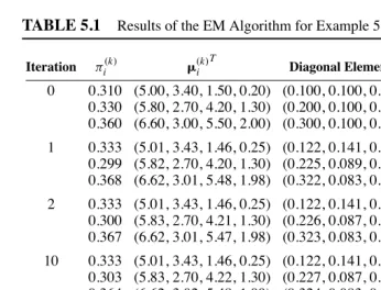
which is obtained through the use of k-means clustering method. With the EMMIX program, the default stopping criterion is that the change in the log likelihood from the current iteration and the log likelihood from 10 iterations previously differs by less than 0.000001 of the current log likelihood [22]. The results of the EM algorithm are presented in Table 5.1. The MLE ofΨcan be taken to be the value ofΨ(k)on iteration
k=29. Alternatively, the EMMIX program offers automatic starting values for the
application of the EM algorithm. As an example, an initial valueΨ(0)is determined
TABLE 5.1
Results of the EM Algorithm for Example 5.1Log Iteration πi(k) (k)i T Diagonal Elements ofΣ(k)i Likelihood
0 0.310 (5.00, 3.40, 1.50, 0.20) (0.100, 0.100, 0.030, 0.010) −317.98421
0.330 (5.80, 2.70, 4.20, 1.30) (0.200, 0.100, 0.200, 0.030) 0.360 (6.60, 3.00, 5.50, 2.00) (0.300, 0.100, 0.300, 0.100)
1 0.333 (5.01, 3.43, 1.46, 0.25) (0.122, 0.141, 0.030, 0.011) −306.90935
0.299 (5.82, 2.70, 4.20, 1.30) (0.225, 0.089, 0.212, 0.034) 0.368 (6.62, 3.01, 5.48, 1.98) (0.322, 0.083, 0.325, 0.088)
2 0.333 (5.01, 3.43, 1.46, 0.25) (0.122, 0.141, 0.030, 0.011) −306.87370
0.300 (5.83, 2.70, 4.21, 1.30) (0.226, 0.087, 0.218, 0.034) 0.367 (6.62, 3.01, 5.47, 1.98) (0.323, 0.083, 0.328, 0.087)
10 0.333 (5.01, 3.43, 1.46, 0.25) (0.122, 0.141, 0.030, 0.011) −306.86234
0.303 (5.83, 2.70, 4.22, 1.30) (0.227, 0.087, 0.224, 0.035) 0.364 (6.62, 3.02, 5.48, 1.99) (0.324, 0.083, 0.328, 0.086)
20 0.333 (5.01, 3.43, 1.46, 0.25) (0.122, 0.141, 0.030, 0.011) −306.86075
0.304 (5.83, 2.70, 4.22, 1.30) (0.228, 0.087, 0.225, 0.035) 0.363 (6.62, 3.02, 5.48, 1.99) (0.324, 0.083, 0.327, 0.086)
29 0.333 (5.01, 3.43, 1.46, 0.25) (0.122, 0.141, 0.030, 0.011) −306.86052
0.305 (5.83, 2.70, 4.22, 1.30) (0.229, 0.087, 0.225, 0.035) 0.362 (6.62, 3.02, 5.48, 1.99) (0.324, 0.083, 0.327, 0.085)
5.4.2
Example 5.2: Mixtures of Factor Analyzers
McLachlan and Peel [21] adopt a mixture of factor analyzers model to cluster the so-called wine data set, which is available at the UCI Repository of machine learning databases [1]. These data give the results of a chemical analysis of wines grown in the same region in Italy, but derived from three different cultivars. The analysis
determined the quantities of p =13 consituents found in each of n = 178 wines.
To cluster this data set, a three-component normal mixture model can be adopted. However, as p=13 in this problem, the (unrestricted) covariance matrixΣihas 91 parameters for each i (i=1,2,3), which means that the total number of parameters is very large relative to the sample size of n = 178. A mixture of factor analyzers can be used to reduce the number of parameters to be fitted. In a mixture of factor analyzers, each observationY jis modeled as
Y j =i+BiUi j+i j
N (0,Di), whereIqis the q×q identity matrix andDiis a p×p diagonal matrix (i =1, . . . ,g). That is,
f (yj;Ψ)= g
i=1
πiφ(yj;i,Σi)
where
Σi =BiBTi +Di (i=1, . . . ,g)
The vector of unknown parametersΨnow consists of the elements of thei, theBi, and theDi, along with the mixing proportionsπi(i =1, . . . ,g−1).
The alternating expectation conditional-maximization (AECM) algorithm [24] can be used to fit the mixture of factor analyzers model by ML; see Section 5.5. The unknown parameters are partitioned as (ΨT
1,Ψ
T
2)
T
, whereΨ1contains theπi (i = 1, . . . ,g−1) and the elements ofi(i =1, . . . ,g). The subvectorΨ2contains the
elements ofBi andDi(i =1, . . . ,g). The AECM algorithm is an extension of the expectation-conditional maximization (ECM) algorithm [23], where the specification of the complete-data is allowed to be different on each conditional maximization (CM) step. In this application, one iteration consists of two cycles corresponding to the partition ofΨintoΨ1andΨ2, and there is one E-step and one CM-step for each
cycle. For the first cycle of the AECM algorithm, we specify the missing data to be just the component-indicator vectors,z1, . . . ,zn; see Equation (5.4). The E-step on the first cycle on the (k+1)th iteration is essentially the same as given in Equations (5.5) and (5.6). The first CM-step computes the updated estimateΨ(k+1)1 as
π(k+1)
i = n
j=1 τ(k)
i j /n
and
(k+1)
i = n
j=1
τ(k)
i j yj/ n
j=1
τ(k)
i j
for i=1, . . . ,g. For the second cycle for the updating ofΨ2, we specify the missing
data to be the factors Ui 1, . . . ,Ui n, as well as the component-indicator vectors, z1, . . . ,zn. On settingΨ(k+1/2)equal to (Ψ(k+1)
1
T
,Ψ(k)2 T)T, the E-step on the second cycle calculates the conditional expectations as
EΨ(k+1/2){Zi j(Ui j−i)|yj} =τi j(k+1/2)(k)i
T
(yj−i)
and
EΨ(k+1/2){Zi j(Ui j−i)(Ui j−i)T|yj}
=τ(k+1/2)
i j
(k)
i T
(yj−i)(yj−i)T(k)i +Ω
(k)
i
where
(k)
i =
B(k)i B
(k)
i T
+D(k)i −1
and
Ω(k)i =Iq−
(k)
i T
B(k)i
for i =1, . . . ,g. The E-step above uses the result that the conditional distribution of Ui jgivenyj and zi j =1 is given by
Ui j|yj,zi j =1∼N
T
i (yj−i),Ωi
for i = 1, . . . ,g; j = 1, . . . ,n. The CM-step on the second cycle provides the updated estimateΨ(k+1)2 as
B(ki +1)=V
(k+1/2)
i
(k)
i
(k)
i T
V(ki +1/2)
(k)
i +Ω
(k)
i −1
and
D(ki +1)= diag
V(k+1i /2)−B
(k+1)
i H
(k+1/2)
i B
(k+1)
i T
where
V(k+1i /2)= n
j=1τ(k+1/ 2)
i j (yj−(k+1)i )(yj−(k+1)i )T n
j=1τ
(k+1/2)
i j
and
Hi(k+1/2)=
(k)
i T
V(k+1i /2)
(k)
i +Ω
(k)
i
As an illustration, a mixture of factor analyzers model with different values of q is fitted to the wine data set, ignoring the known classification of the data. To determine
the initial estimate of Ψ, the EMMIX program is used to fit the normal mixture
model with unrestricted component-covariance matrices using ten random starting values (with 70% subsampling of the data). The estimates ofπi andi so obtained
are used as the initial values for πi andi in the AECM algorithm. The estimate
ofΣi so obtained (denoted asΣ(0)i ) is used to determine the initial estimate ofDi, whereD(0)i is taken to be the diagonal matrix formed from the diagonal elements of Σi(0). An initial estimate ofBi can be obtained using the method described in [20].
The results of the AECM algorithm from q=1 to q =8 are presented in Table 5.2.
We have also reported the value of minus twice the likelihood ratio test statisticλ (i.e., twice the increase in the log likelihood), as we proceed from fitting a mixture of q factor analyzers to one with q+1 component factors. For a given level of the number of components g, regularity conditions hold for the asymptotic null distribution of
−2 logλ to be chi-squared with d degrees of freedom, where d is the difference
between the number of parameters under the null and alternative hypotheses for the value of q. It can be seen from Table 5.2 that the apparent error rate of the outright
clustering is smallest for q = 2 and 3. However, this error rate is unknown in a
clustering context and so cannot be used as a guide to the choice of q. Concerning the use of the likelihood ratio test to decide on the number of factors q, the test of q =q0=6 versus q=q0+1=7 is not significant (P=0.28), on taking−2 logλto
be chi-squared with d=g( p−q0)=21 degrees of freedom under the null hypothesis
TABLE 5.2
Results of the AECM Algorithm for Example 5.2 q Log Likelihood Error (%Error) −2 log1 −3102.254 2 (1.12) —
2 −2995.334 1 (0.56) 213.8
3 −2913.122 1 (0.56) 164.4
4 −2871.655 3 (1.69) 82.93
5 −2831.860 4 (2.25) 79.59
6 −2811.290 4 (2.25) 41.14
7 −2799.204 4 (2.25) 24.17
8 −2788.542 4 (2.25) 21.32
5.5
Advanced Topics
In this section, we consider some extensions of the EM algorithm to handle problems with more difficult E-step and/or M-step computations, and to tackle problems of slow convergence. Moreover, we present a brief account of the applications of the EM algorithm in the context of Hidden Markov Models (HMMs), which provide a convenient way of formulating an extension of a mixture model to allow for dependent data.
In some applications of the EM algorithm such as with generalized linear mixed models, the E-step is complex and does not admit a close-form solution to the Q-function. In this case, the E-step may be executed by a Monte Carlo (MC) process. At the (k+1)th iteration, the E-step involves
r simulation of M independent sets of realizations of the missing dataZfrom
the conditional distribution g(z|y;Ψ(k))
r approximation of the Q-function by
Q(Ψ;Ψ(k))≈QM(Ψ;Ψ(k))= 1
M M
m=1
log Lc(Ψ;y,z(mk))
wherez(mk)is the mth set of missing values based onΨ(k)
In the M-step, the Q-function is maximized overΨto obtainΨ(k+1). This variant is
known as the Monte Carlo EM (MCEM) algorithm [33]. As an MC error is introduced at the E-step, the monotonicity property is lost. But in certain cases, the algorithm gets close to a maximizer with a high probability [4]. The problems of specifying M and monitoring convergence are of central importance in the routine use of the algorithm; see [4, 18, 33].
The ECM algorithm [23] is a natural extension of the EM algorithm in situations where the maximization process on the M-step is relatively simple when conditional on some function of the parameters under estimation. The ECM algorithm takes advantage of the simplicity of complete-data conditional maximization by replacing a complicated M-step of the EM algorithm with several computationally simpler CM steps. In particular, the ECM algorithm preserves the appealing convergence properties of the EM algorithm [18, 23]. The AECM algorithm [24] mentioned in Section 5.4.2 allows the specification of the complete-data to vary where necessary over the CM-steps within and between iterations. This flexible data augmentation and model reduction scheme is eminently suitable for applications like mixtures of factor analyzers where the parameters are large in number.
Massively huge data sets of millions of multidimensional observations are now commonplace. There is an ever increasing demand on speeding up the convergence of the EM algorithm to large databases. But at the same time, it is highly desirable if its simplicity and stability can be preserved. An incremental version of the EM algorithm was proposed by Neal and Hinton [25] to improve the rate of convergence of the EM algorithm. This incremental EM (IEM) algorithm proceeds by dividing the data into B blocks and implementing the (partial) E-step for only a block of data at a time before performing an M-step. That is, a “scan” of the IEM algorithm consists of B partial E-steps and B full M-steps [26]. It can be shown from Exercises 6 and 7 in Section 5.6 that the IEM algorithm in general converges with fewer scans and hence faster than the EM algorithm. The IEM algorithm also increases the likelihood at each scan; see the discussion in [27].
In the mixture framework with observations y1, . . . ,yn, the unobservable
component-indicator vectorz =(zT
1, . . . ,z
T n)
T
can be termed as the “hidden vari-able.” In speech recognition applications, thezjmay be unknown serially dependent prototypical spectra on which the observed speech signalsyjdepend ( j=1, . . . ,n). Hence the sequence or set of hidden valueszjcannot be regarded as independent. In the automatic speech recognition applications or natural language processing (NLP) tasks, a stationary Markovian model over a finite state space is generally formulated for the distribution of the hidden variableZ[18]. As a consequence of the dependent
structure of Z, the density of Yj will not have its simple representation
[Equa-tion (5.1)] of a mixture density as in the independence case. However,Y1, . . . ,Yn are assumed conditionally independent givenz1, . . . ,zn; that is
f (y1, . . . ,yn|z1, . . . ,zn;)=
n
j=1
f (yj|zj;)
wheredenotes the vector containing the unknown parameters in these conditional
can be implemented in closed form, using formulas which are a combination of the MLEs for the multinomial parameters and Markov chain transition probabilities; see [14, 30].
5.6
Exercises
Ten exercises are given in this section. They arise in various scientific fields in the contexts of data mining and pattern recognition, in which the EM algorithm or its variants have been applied. The exercises include problems where the incompleteness of the data is perhaps not as natural or evident as in the two illustrative examples in Section 5.4.
1. B¨ohning et al. [3] consider a cohort study on the health status of 602 preschool children from 1982 to 1985 in northest Thailand [32]. The frequencies of illness spells (fever, cough, or both) during the study period are presented in Table 5.3. A three-component mixture of Poisson distributions is fitted to the data. The log likelihood function is given by
log L(Ψ)= n
j=1
log 3
i=1
πif (yj, θi)
whereΨ=(π1, π2, θ1, θ2, θ3)Tand
f (yj, θi)=exp(−θi)θ yj
i /yj! (i =1,2,3)
With reference to Section 5.4.1, let
τi(yj;Ψ(k))=πi(k)f
yj, θi(k)
3
h=1 π(k)
h f
yj, θh(k)
(i=1,2,3)
denote the posterior probability that yj belongs to the i th component. Show that the M-step updates the estimates as
πi(k+1) = n
j=1
τi(yj;Ψ(k))/n (i=1,2)
θi(k+1) = n
j=1
τi(yj;Ψ(k))yj/
nπi(k+1)
(i =1,2,3)
Using the initial estimatesπ1=0.6,π2 =0.3,θ1 =2,θ2 =9, andθ3 =17,
TABLE 5.3
Frequencies of Illness Spells for a Cohort Sample of Preschool Children in Northest ThailandNo. of No. of No. of
Illnesses Frequency Illnesses Frequency Illnesses Frequency
0 120 8 25 16 6
1 64 9 19 17 5
2 69 10 18 18 1
3 72 11 18 19 3
4 54 12 13 20 1
5 35 13 4 21 2
6 36 14 3 23 1
7 25 15 6 24 2
2. The fitting of mixtures of (multivariate) t distributions was proposed by McLachlan and Peel [19] to provide a more robust approach to the fitting of normal mixture models. A g-component mixture of t distributions is given by
f (yj;Ψ)= g
i=1
πif (yj;i,Σi, νi)
where the component density f (yj;i,Σi, νi) has a multivariate t distribution with locationi, positive definite inner product matrixΣi, andνi degrees of freedom (i =1, . . . ,g); see [19, 29]. The vector of unknown parameters is
Ψ=(π1, . . . , πg−1,T,T)T
where=(ν1, . . . , νg)Tare the degrees of freedom for the t distributions, and
=(T
1, . . . ,
T g)
T, and where
i contains the elements ofi and the distinct elements ofΣi (i =1, . . . ,g). With reference to Section 5.4.1, the observed data augmented by the component-indicator vectorsz1, . . . ,znare viewed as still being incomplete. Additional missing data, u1, . . . ,un, are introduced into the complete-data vector, that is,
x=yT,zT
1, . . . ,z
T
n,u1, . . . ,un T
where u1, . . . ,unare defined so that, given zi j=1,
Yj|uj,zi j =1∼N (i,Σi/uj)
independently for j =1, . . . ,n, and
Uj|zi j=1∼ gamma 1
2νi, 1 2νi
Show that the complete-data log likelihood can be written in three terms as
where
log L1c()=
g
i=1
n
j=1
zi jlogπi
log L2c()=
g i=1 n j=1
zi j−log (12νi)+12νilog(12νi)+12νi(log uj−uj)−log uj
and
log L3c()=
g i=1 n j=1
zi j−12p log(2π)−12log|Σi| −12ujδ(yj,i,;Σi)
where
δ(yj,i;Σi)=(yj−i) T
Σ−1i (yj−i)
3. With reference to the above mixtures of t distributions, show that the E-step on the (k+1)th iteration of the EM algorithm involves the calculation of
EΨ(k)(Zi j|y) = τi j(k)= π(k)
i f (yj;
(k)
i ,Σ
(k)
i , ν
(k)
i ) f (yj;Ψ(k))
(5.11)
EΨ(k)(Uj|y,zi j = 1)=ui j(k)= ν (k)
i +p
ν(k)
i +δ(yj,
(k)
i ; Σ
(k)
i )
(5.12)
and
EΨ(k)(log Uj|y,zi j=1)=log u(k)i j +
ψ
ν(k)
i +p 2
−log
ν(k)
i +p 2
(5.13)
for i =1, . . . ,g; j=1, . . . ,n. In Equation (5.13),
ψ(r )= {∂ (r )/∂r}/ (r )
is the Digamma function [29]. Hint for Equation (5.12): the gamma distribution is the conjugate prior distribution for Uj; Hint for Equation (5.13): if a random variable S has a gamma(α, β) distribution, then
E(log S)=ψ(α)−logβ.
Also, it follows from Equation (5.10) that (k+1),(k+1), and(k+1) can be
computed on the M-step independently of each other. Show that the updating formulas for the first two are
πi(k+1) = n
j=1
τ(k)
i j /n
(k+1)i = n
j=1 τ(k)
i j u
(k)
i jyj
n
j=1 τ(k)
i j u
(k)
and
Σ(k+1)i = n
j=1τ
(k)
i j u
(k)
i j(yj−(k+1)i )(yj−(k+1)i )T n
j=1τ (k)
i j
The updatesνi(k+1)for the degrees of freedom need to be computed iteratively. It follows from Equation (5.10) thatνi(k+1)is a solution of the equation
−ψ1
2νi
+log12νi
+1+n1(k)
i
n j=1τ
(k)
i j
log u(k)i j −u
(k)
i j
+ψ
ν(k)
i +p 2
−log
ν(k)
i +p 2
=0
where n(k)i = n
j=1τ
(k)
i j (i=1, . . . ,g).
4. The EMMIX program [22] has an option for the fitting of mixtures of multi-variate t components. Now fit a mixture of two t components (with unrestricted scale matricesΣiand unequal degrees of freedomνi) to the Leptograpsus crab data set of Campbell and Mahon [5]. With the crab data, one species has been split into two new species, previously grouped by color form, orange and blue. Data are available on 50 specimens of each sex of each species. Attention here
is focussed on the sample of n =100 five-dimensional measurements on
or-ange crabs (the two components correspond to the males and females). Run the EMMIX program with automatic starting values from 10 random starts (using 100% subsampling of the data), 10 k-means starts, and 6 hierarchical methods (with user-supplied initial valuesν1(0)=ν2(0)=13.193 which is obtained in the case of equal scale matrices and equal degrees of freedom). Verify estimates of
are ˆν1=12.2 and ˆν2 =300.0 and the numbers assigned to each component are, respectively, 47 and 53 (misclassification rate=3%).
5. For a mixture of g component distributions of generalized linear models (GLMs) in proportions π1, . . . , πg, the density of the j th response variable Yjis given by
f (yj;Ψ)= g
i=1
πif (yj;θi j, κi)
where the log density for the i th component is given by
log f (yj;θi j, κi)=κi−1{θi jyj−b(θi j)} +c(yj;κi) (i=1, . . . ,g)
whereθi jis the natural or canonical parameter andκiis the dispersion parameter. For the i th component GLM, denoteμi jthe conditional mean of Yjandηi j = hi(μi j) = T
i xj the linear predictor, where hi(·) is the link function andxj is a vector of explanatory variables on the j th response yj [20]. The vector of unknown parameters isΨ=(π1, . . . , πg−1, κ1, . . . , κg, T1, . . . , Tg)
T. Let
component densitiesφ(yj;i,Σi) replaced by f (yj;θi j, κi). On the M-step, the updating formula forπi(k+1)(i =1, . . . ,g−1) is
πi(k+1)= n
j=1
τ(k)
i j /n
where
τ(k)
i j =π
(k)
i f
yj;θi j(k), κ
(k)
i
g
h=1
π(k)
h f
yj;θh j(k), κ
(k)
h
The updatesκi(k+1)and (k+1)i need to be computed iteratively by solving
n
j=1 τ(k)
i j ∂log f (yj;θi j, κi)/∂κ = 0
n
j=1
τ(k)
i j ∂log f (yj;θi j, κi)/∂ i = 0 (5.14)
Consider a mixture of gamma distributions, where the gamma density function for the i th component is given by
f (yj;μi j, αi)= (αi
μi j)
αiy(αi−1)
j exp(−μαi ji yj) (αi)
whereαi >0 is the shape parameter, which does not depend on the explanatory variables. The linear predictor is modelled via a log-link as
ηi j =hi(μi j)=logμi j = Tixj
With reference to Equation (5.14), show that the M-step for a mixture of gamma distributions involves solving the nonlinear equations
n
j=1 τ(k)
i j {1+logαi−logμi j+log yj−yj/μi j−ψ(αi)} = 0,
n
j=1 τ(k)
i j (−1+yj/μi j)αixj =0
whereψ(r )= {∂ (r )/∂r}/ (r ) is the digamma function.
the sufficient statistics for the (b+1)th block (b=0, . . . ,B−1; q=1,2,3). For example,
T(k+i 1,bb+1/B)=
j∈Sb
τi(yj;Ψ(k+b/B)) (i =1, . . . ,g)
where Sb is a subset of{1, . . . ,n}containing the subscripts of thoseyj that belong to the (b+1)th block (b =0, . . . ,B−1). From Equations (5.7) and (5.8), show that the M-step on the (b+1)th iteration of the (k+1)th scan of the IEM algorithm involves the update of the estimates of πi,i, andΣi as follows:
π(k+(b+1)/B)
i = T(k+ b/B) i 1 /n
(k+(b+1)/B) i =T
(k+b/B) i 2 /T
(k+b/B) i 1
Σ(k+(b+1)i /B) =
Ti 3(k+b/B)−Ti 1(k+b/B)−1Ti 2(k+b/B)T(k+i 2 b/B)T /Ti 1(k+b/B)
for i =1, . . . ,g, where
T(k+i q b/B)=T(k+(b−1)/ B)
i q −T(k−1+ b/B) i q,b+1 +T(k+
b/B)
i q,b+1 (5.15)
for i =1, . . . ,g and q=1,2,3. It is noted that the first and second terms on the right-hand side of Equation (5.15) are already available from the previous iteration and the previous scan, respectively. In practice, the IEM algorithm is implemented by running the standard EM algorithm for the first few scans to avoid the “premature component starvation” problem [26]. In this case, we have
T(k)i q = B
b=1
Ti q(k),b (i =1, . . . ,g; q=1,2,3)
7. With the IEM algorithm, Ng and McLachlan [26] provide a simple guide for choosing the number of blocks B for normal mixtures. In the case of component-covariance matrices specified to be diagonal (such as in Example 5.1), they suggest B≈n1/3. For the Iris data in Example 5.1, it implies that B≈(150)1/3. Run an IEM algorithm to the Iris data with B =5 and the same initial values of Ψas in Example 5.1. Verify that (a) the final estimates and the log likelihood value are approximately the same as those using the EM algorithm, and (b) the IEM algorithm converges with fewer scans than the EM algorithm and increases the likelihood at each scan; see the discussion in [27].
contributions of the various experts, whereis a vector of unknown parameters in the gating network. The final output of the ME network is a weighted sum of all the output vectors produced by the expert networks,
f (yj|xj;Ψ)= M
h=1
πh(xj;) fh(yj|xj;h)
Within the incomplete-data framework of the EM algorithm, we introduce the indicator variables Zh j, where zh j is 1 or 0 according to whetheryjbelongs or does not belong to the hth expert. Show that the complete-data log likelihood forΨis given by
log Lc(Ψ)= n
j=1
M
h=1
zh j{logπh(xj;)+log fh(yj|xj;h)}
and the Q-function can be decomposed into two terms with respect toand
h(h=1, . . . ,M), respectively, as
Q(Ψ;Ψ(k))=Q+Q
where
Q = n
j=1 M
h=1
τ(k)
h j logπh(xj;)
Q =
n
j=1
M
h=1 τ(k)
h j log fh(yj|xj;h)
and where
τ(k)
h j =πh(xj;(k)) fh
yj|xj;(k)h
M
r=1
πr(xj;(k)) fr
yj|xj;r(k)
9. With the ME networks above, the output of the gating network is usually modeled by the multinomial logit (or softmax) function as
πh(xj;)=
exp(vT hxj) 1+rM=1−1exp(vT
rxj)
(h=1, . . . ,M−1)
andπM(xj;)=1/(1+rM=1−1exp(v T
rxj)). Herecontains the elements in vh(h=1, . . . ,M−1). Show that the updated estimate of(k+1)on the M-step is obtained by solving
n
j=1
τ(k)
h j −
exp(vT hxj) 1+rM=−11 exp(vrTxj)
for h =1, . . . ,M−1, which is a set of nonlinear equations. It is noted that the nonlinear equation for the hth expert depends not only on the parameter vector vh, but also on other parameter vectors in. In other words, each parameter
vectorvhcannot be updated independently. With the IRLS algorithm presented
in [12], the independence assumption on these parameter vectors was used implicitly. Ng and McLachlan [28] propose an ECM algorithm for which the
M-step is replaced by (M−1) computationally simpler CM-steps forvh(h=
1, . . . ,M−1).
10. McLachlan and Chang [17] consider the mixture model-based approach to the cluster analysis of mixed data, where the observations consist of both continu-ous and categorical variables. Suppose that p1of the p feature variables inY j are categorical, where the qth categorical variable takes on mqdistinct values (q =1, . . . ,p1). With the location model-based cluster approach [20], the p1
categorical variables are uniquely transformed to a single multinomial random variableUwith S cells, where S=p1
q=1mqis the number of distinct patterns (locations) of the p1categorical variables. We let (uj)sbe the label for the sth location of the j th entity (s =1, . . . ,S; j =1, . . . ,n), where (uj)s =1 if the realizations of the p1 categorical variables correspond to the sth pattern,
and is zero otherwise. The location model assumes further that conditional on (uj)s =1, the conditional distribution of the p−p1continuous variables is
normal with meani sand covariance matrixΣi, which is the same for all S
cells. Let pi s be the conditional probability that (Uj)s = 1 given its mem-bership of the i th component of the mixture (s = 1, . . . ,S; i = 1, . . . ,g). With reference to Section 5.4.1, show that on the (k+1)th iteration of the EM algorithm, the updated estimates are given by
π(k+1)
i = S
s=1
n
j=1 δj sτi j s(k)
n
p(k+1)i s = n
j=1
δj sτi j s(k)
S
r=1 n
j=1
δjrτi jr(k)
(k+1)i s = n
j=1
δj sτi j s(k)y∗j
n
j=1
δj sτi j s(k)
and
Σ(k+1)i = S s=1 n j=1
δj sτi j s(k)
y∗j−(k+1)i s
y∗j−(k+1)i s T S s=1 n j=1
δj sτi j s(k)
whereδj sis 1 or 0 according as to whether (uj)sequals 1 or 0,y∗jcontains the continuous variables inyj, and
τ(k)
i j s =π
(k)
i p
(k)
i sφ
y∗j;
(k)
i s,Σ
(k) i g h=1 π(k) h p (k) hsφ
y∗j;
(k)
hs,Σ
(k)
h
References
[1] A. Asuncion and D.J. Newman. UCI Machine Learning Repository. University
of California, School of Information and Computer Sciences, Irvine, 2007. http://www.ics.uci.edu/ mlearn/MLRepository.html.
[2] L.E. Baum, T. Petrie, G. Soules, and N. Weiss. A maximisation technique
occurring in the statistical analysis of probabilistic functions of Markov process. Annals of Mathematical Statistics, 41:164–171, 1970.
[3] D. B¨ohning, P. Schlattmann, and B. Lindsay. Computer-assisted analysis of
mixtures (C.A.MAN): Statistical algorithms. Biometrics, 48:283–303, 1992.
[4] J.G. Booth and J.P. Hobert. Maximizing generalized linear mixed model
like-lihoods with an automated Monte Carlo EM algorithm. Journal of the Royal Statistical Society B, 61:265–285, 1999.
[5] N.A. Campbell and R.J. Mahon. A multivariate study of variation in two species
of rock crab of genus Leptograpsus. Australian Journal of Zoology, 22:417– 425, 1974.
[6] D.R. Cox and D. Hinkley. Theoretical Statistics. Chapman & Hall, London,
1974.
[7] H. Cram´er. Mathematical Methods of Statistics. Princeton University Press,
New Jersey, 1946.
[8] A.P. Dempster, N.M. Laird, and D.B. Rubin. Maximum likelihood from
in-complete data via the EM algorithm. Journal of the Royal Statistical Society B, 39:1–38, 1977.
[9] C. Fraley and A.E. Raftery. Mclust: Software for model-based cluster analysis.
Journal of Classification, 16:297–306, 1999.
[10] R.A. Jacobs, M.I. Jordan, S.J. Nowlan, and G.E. Hinton. Adaptive mixtures of
local experts. Neural Computation, 3:79–87, 1991.
[11] M. Jamshidian and R.I. Jennrich. Standard errors for EM estimation. Journal
of the Royal Statistical Society B, 62:257–270, 2000.
[12] M.I. Jordan and R.A. Jacobs. Hierarchical mixtures of experts and the EM
algorithm. Neural Computation, 6:181–214, 1994.
[13] E.L. Lehmann and G. Casella. Theory of Point Estimation. Springer-Verlag,
New York, 2003.
[14] B.G. Leroux and M.L. Puterman. Maximum-penalized-likelihood estimation
for independent and Markov-dependent mixture models. Biometrics, 48:545– 558, 1992.
[15] T.A. Louis. Finding the observed information matrix when using the EM
[16] G.J. McLachlan and K.E. Basford. Mixture Models: Inference and Applications to Clustering. Marcel Dekker, New York, 1988.
[17] G.J. McLachlan and S.U. Chang. Mixture modelling for cluster analysis.
Sta-tistical Methods in Medical Research, 13:347–361, 2004.
[18] G.J. McLachlan and T. Krishnan. The EM Algorithm and Extensions (2nd
edition). Wiley, New Jersey, 2008.
[19] G.J. McLachlan and D. Peel. Robust cluster analysis via mixtures of
multi-variate t-distributions. In Lecture Notes in Computer Science, pages 658–666. Springer-Verlag, Berlin, 1998. Vol. 1451.
[20] G.J. McLachlan and D. Peel. Finite Mixture Models. Wiley, New York, 2000.
[21] G.J. McLachlan and D. Peel. Mixtures of factor analyzers. In P. Langley, editor, Proceedings of the 17th International Conference on Machine Learning, pages 599–606, San Francisco, 2000. Morgan Kaufmann.
[22] G.J. McLachlan, D. Peel, K.E. Basford, and P. Adams. The emmix software
for the fitting of mixtures of normal and t-components. Journal of Statistical Software, 4:No. 2, 1999.
[23] X.-L. Meng and D. Rubin. Maximum likelihood estimation via the ECM
algo-rithm: A general framework. Biometrika, 80:267–278, 1993.
[24] X.-L. Meng and D.A. van Dyk. The EM algorithm—an old folk song sung to
a fast new tune. Journal of the Royal Statistical Society B, 59:511–567, 1997.
[25] R.M. Neal and G.E. Hinton. A view of the EM algorithm that justifies
incre-mental, sparse, and other variants. In M.I. Jordan, editor, Learning in Graphical Models, pages 355–368. Kluwer, Dordrecht, 1998.
[26] S.K. Ng and G.J. McLachlan. On the choice of the number of blocks with the
incremental EM algorithm for the fitting of normal mixtures. Statistics and Computing, 13:45–55, 2003.
[27] S.K. Ng and G.J. McLachlan. Speeding up the EM algorithm for mixture
model-based segmentation of magnetic resonance images. Pattern Recogni-tion, 37:1573–1589, 2004.
[28] S.K. Ng and G.J. McLachlan. Using the EM algorithm to train neural
net-works: Misconceptions and a new algorithm for multiclass classification. IEEE Transactions on Neural Networks, 15:738–749, 2004.
[29] D. Peel and G.J. McLachlan. Robust mixture modelling using the t distribution. Statistics and Computing, 10:335–344, 2000.
[30] L.R. Rabiner. A tutorial on hidden Markov models and selected applications in
speech recognition. Proceedings of the IEEE, 77:257–286, 1989.
[32] F.-P. Schelp, P. Vivatanasept, P. Sitaputra, S. Sormani, P. Pongpaew, N. Vudhivai, S. Egormaiphol, and D. B¨ohning. Relationship of the morbidity of under-fives to anthropometric measurements and community health inter-vention. Tropical Medicine and Parasitology, 41:121–126, 1990.
[33] G.C.G. Wei and M.A. Tanner. A Monte Carlo implementation of the EM