Limit sets and switching strategies in parameter-optimal iterative learning control

This is a repository copy of Limit sets and switching strategies in parameter-optimal

iterative learning control.

White Rose Research Online URL for this paper:

http://eprints.whiterose.ac.uk/74689/

Monograph:

Owens, D.H., Tomas-Rodriguez, M. and Daley, S. (2007) Limit sets and switching

strategies in parameter-optimal iterative learning control. Research Report. ACSE

Research Report no. 943 . Automatic Control and Systems Engineering, University of

Sheffield

[email protected] https://eprints.whiterose.ac.uk/ Reuse

Unless indicated otherwise, fulltext items are protected by copyright with all rights reserved. The copyright exception in section 29 of the Copyright, Designs and Patents Act 1988 allows the making of a single copy solely for the purpose of non-commercial research or private study within the limits of fair dealing. The publisher or other rights-holder may allow further reproduction and re-use of this version - refer to the White Rose Research Online record for this item. Where records identify the publisher as the copyright holder, users can verify any specific terms of use on the publisher’s website.

Takedown

If you consider content in White Rose Research Online to be in breach of UK law, please notify us by

Limit Sets and Switching Strategies in Parameter-Optimal

Iterative Learning Control

D H Owens, M Tomas-Rodriguez, S.Daley

Department of Automatic Control and Systems Engineering,

University of Sheffield,

Mappin Street, Sheffield S1 3JD, United Kingdom

Email: [email protected]

February 8, 2007

Abstract

This paper characterizes the existence and form of the possible limit error signals in typical parameter-optimal Iterative Learning Control. The set of limit errors has attracting and repelling components and the behaviour of the algorithm in the vicinity of these sets can be associated with the undesirable properties of apparent (but in fact temporary) convergence or permanent slow convergence properties in practice. The avoidance of these behaviours in practice is investigated using novel switching strategies. Deterministic strategies are analysed to prove the feasibility of the concept by proving that each of a number of such strategies is guaranteed to produce global convergence of errors to zero independent of the details of plant dynamics. For practical applications a random switching strategy is proposed to replace these approaches and shown, by example, to produce substantial potential improvements when compared with the non-switching case. The work described in this paper is covered by pending patent applications in the UK and elsewhere.

Keywords: Iterative learning control, robust control, nonlinear control, positive-real systems, switching control, optimization

1

Introduction

Iterative Learning Control (ILC) is concerned with the performance of systems that operate in a

repet-itive manner and includes examples such as robot arm manipulators and chemical batch processes,

high precision. The use of conventional control algorithms with such systems will, in the absence of

noise or disturbance, result in the same level of tracking error being repeated time and time again.

Mo-tivated by human learning, ILC uses information from previous executions of the task in an attempt

to improve performance from repetition to repetition in the sense that the tracking error (between the

output and a specified reference trajectory) is sequentially reduced to zero (see, for example, [1], [2]

and the recent reviews [3], [6]. Note that repetitions are often called trials, passes or iterations in the

literature.

This first part of this paper is concerned with the analysis of the limiting behaviour of

Parameter-Optimal Iterative Learning Control POILC introduced in Owens and Feng [4] and its generalization

[5]. This extends the results in [7] and forms a motivation for the second part. The second part

presents a new switching-based approach to eliminate undesirable effects of such limiting behaviour.

In [4], the discrete time, linear case is considered and the behaviour of a simple feedforward ILC

algorithm is analysed in detail. The algorithm operates with a learning gain updated from trial to

trial through the minimization of a quadratic performance index. Despite its simplicity the algorithm

has the powerful property of ensuring that the mean square error (Euclidean norm) of the error time

series reduces from trial to trial . The important property of guaranteed convergence to a zero tracking

error is seen to depend critically upon positivity of a plant matrix description (or, more generally, the

positivity of the representation of a compensated plant). If the positivity condition is not satisfied,

convergence to a non-zero limit error is always a realistic possibility and can be seen in practice.

For the Owens and Feng algorithm, the form of the set of limit errors (the so-called limit setS∞)

is characterized as the points (error time series) where a certain quadratic form vanishes. This divides

the error time series space into three components - the limit set and two open sets (one of which

is convex). Based upon properties observed during simulation studies, the authors initiated (in [7])

a theoretical study of the phenomenon reported. In that publication, the limit set is shown to have

interesting implications for POILC algorithm performance, namely

1. It is shown that the limit setS∞, in general, will have attractingS∞− and repelling components

S+∞(i.e. it has internal structure) and that

2. the behaviour of the algorithm in the vicinity of the repelling componentS∞+ is associated with

temporary slow convergence (which may tempt the user to believe, erroneously, that

conver-gence has occurred) whilst

3. close to the attracting componentS−

S− ∞.

4. Moreover, close to the repelling part of the limit set, the behaviour of the POILC algorithm is

highly sensitive to small variations in the initial error time series.

Sufficient conditions to characterize the attracting and repelling components of the limits set are

derived in [7]. This paper extends these results to provide precise necessary and sufficient conditions.

The ideas are illustrated by graphical analysis of a simple example in_R2 (representing times series

with only two elements). Although not a practical example (as time series will, in general have

hundreds or thousands of data points), this simple case provides an indication of the phenomena

summarised above and are included to motivate the switching concepts used later in the paper. A

simple example using more realistic data sizes is seen to exhibit the temporary slow convergence

property so it is believed that it is an issue that truly has practical implications. The authors argue

that it is hence important to understand these issues theoretically and to look for theoretically sound

approaches to eliminate or reduce the problem in practice.

The paper then considers the fundamental question of whether or not the ILC algorithm can be

modified to eliminate the problems and ensure that convergence to a non-zero element of the limit set

is replaced by a guarantee of convergence to a zero limit error. The innovative approach suggested

is to avoid these behaviours by incorporating a switching strategy into the algorithm. The intuition

behind the approach is that appropriate switching will cause the limit set to change constantly. In such

circumstances it is possible that a monotonically reducing error cannot then converge to a non-zero

limit leaving zero as the only other possibility. The existence of deterministic switching strategies

is shown firstly through a dense search argument and then by switching through a sufficiently large

set of data filters. Analysis proves convergence of errors to zero in both cases but the approaches are

seen to have a large number of degrees of freedom. As a consequence an empirical random switching

strategy is proposed. No analysis is provided but computational studies are presented that indicate

that the most probable outcome is a substantial improvements when compared with the non-switching

case. The paper concludes with a brief discussion of the possibilities for further work in the area.

2

Problem definition

Consider a standard discrete-time,linear, time-invariant single-input, single-output state-space

repre-sentation defined over afinite, discretetime interval, t _∈ [0, N](in order to simplify notation it is

mode where at the end of each repetition, the state is reset to a specified initial conditionx0 for the

next operation during which a new control input signal can be used. A reference signalr(t)is

spec-ified and the ultimate control objective is to find an input functionu∗_{(t)so that the resultant output}

functiony(t)tracks this reference signalr(t)exactlyon[0, N]. The process model is written in the

form:

x(t+ 1) =Ax(t) +Bu(t), x(0) =x0

y(t) =Cx(t) +Du(t)

(1)

where the statex(_·) _∈ Rn, outputy(_·) _∈ Rand inputu(_·) _∈ R. The matricesA, BandC have an appropriate dimensions andDis a scalar. It will be assumed that eitherD₆= 0orCAj−1B ₆= 0for somej = k∗ ₌

≥ 1(trivially satisfied in practice) and that the system (1) is both controllable and

observable. IfD ₆= 0, then takek∗ = 0. By construction, k∗ is the relative degree of the transfer functionG(z) = C(zI₋A)−1_{B+Dof the system. For notational conveniencef}

k(t)will denote

the value of a signal at timeton iterationk.

The repetitive nature of the problem permits the iterative modification of the input functionu(t)

so that, as the number of repetitions increases, the system asymptotically learns the input function

that gives perfect tracking. More precisely, the control objective is to find a causal recursive control

law

uk+1(t) =f(uk(·), uk−1(·), . . . uk−r(·), ek+1(·), ek(·), . . . , ek−s(·)) (2)

with the properties that, independent of the control input time series chosen for the first trial,

limk→∞kek(·)k= 0 limk→∞kuk(·)−u∗(·)k= 0 (3)

where_{k · k}denotes any norm for the time series. In what follows, this norm is taken to be the mean

square error of the time series which is just the Euclidean norm of the vector of the time series. Other

design issues of rate of convergence, robustness etc are also important to practical application but are

not relevant to the main results of this paper and will be pursued in future research.

3

Matrix Representations of Plant Dynamics

The state space model is a natural description for the process. For this paper, an equivalent matrix

description is the preferred method of analysis as it allows a more compact description of the

theo-retical results and releases methods of matrix algebra for analysis. This idea has been used elsewhere

([4]-[7] and by other authors) but the key concepts and notation are included for completeness and

series. It follows that, on finite time intervals, there exists a matrix relating these time series. This

matrix is an equivalent description of systems dynamics.

To construct this matrix model in_RN+1, define the time series "super-vectors" on thekth_{trial via}

uk = [uk(0), uk(1), . . . , uk(N)]T (4)

yk= [yk(0), yk(1), . . . , yk(N)]T (5)

ek= [ek(0), ek(1), . . . , ek(N)]T. (6)

whereek(j) = r(j)−yk(j),0 ≤j ≤N. Furthermore, letu∗be the input sequence (in time series

or supervector form) that givesr(t) = [Gcu∗](t)andGcis the convolution mapping corresponding

to (1).

Note that if the mapping f in (2) is not a function of ek+1, then it is typically said that the

algorithm is offeedforwardtype. If it does not depend on any of theej,0 ≤j ≤k, it is of feedback

type. Otherwise it is offeedback plus feedforwardtype. In this paper, it is assumed that all feedback

components of the control law have been incorporated into the underlying state space model and

hence that the ILC law is a feedforward law.

With the above definitions, the usual formulae for the input-output response of the system can be

written in the form,k_≥0,

yk=Geuk+d0 (7)

where Ge has dimension (N + 1)×(N + 1) and the lower triangular band structure (Ge)ij =

Ge)(i+1)(j+1) that is required by causality and time invariance of linear time-invariant convolution

systems i.e.

Ge=

           

D 0 0 . . . 0

CB D 0 . . . 0

CAB CB D . . . 0

..

. ... ... . .. ...

CAN−1_{B CA}N−2_{B . . . . . . D}             (8)

Alsod0 = [Cx0, CAx0, ..., CANx0]T.

The elementsCAj_{B of the matrixG}

eare the Markov parameters of the plant (1). Assume from

now on that the plant transfer functionG(z) = C(zI₋A)−1B +Dhas relative degree (pole-zero excess)k∗

≥0. Assume also that the reference signalr(t)satisfiesr(j) =CAj_x

0 for0 ≤j < k∗

it is sufficient to analyse a ’lifted’ plant equation that is just the above ifk∗_{= 0or, ifk}∗

≥1,

yk,l =Ge,luk,l+d1 (9)

whereuk,l = [uk(0), uk(1), . . . , uk(N −k∗)]T,yk,l = [yk(k∗)yk(2) . . . yk(N)]T etc and

Ge,l=

           

CAk∗₋₁

B 0 0 . . . 0

CAk∗

B CAk∗₋₁

B 0 . . . 0

CAk∗+1B CAk∗B CAk∗−1B . . . 0

..

. ... ... . .. ...

CAN−k∗

B CAN−k∗−1_{B . . . . . . CA}k∗−1_B             (10)

andd1 = [CAk∗x0, ..., CANx0]T. For notational convenience, the model is written in all cases

k∗

≥0in the simplified notational form

yk=Guk+d (11)

which has the structure of discrete dynamics in_RN+1−k∗. Note thatGis invertible by construction which confirms that, for an arbitrary referencer on 0 _≤ j _≤ N, there exists a time series u∗ _on 0_≤j_≤(N+ 1₋k∗_{)such thatr =Gu}∗_+donk∗

≤j_≤N. From now on this lifted plant model

will be used as a starting point for analysis.

This result is valuable for this paper which considers the basic algorithm described by the

feed-forwardILC update rule

uk+1=uk+Kek, K∈ R(N+1−k

∗_)×(N+1−k∗₎

(12)

Note:in element by element form, this relation is simply

uk+1(t) =uk(t) + ΣN+1−k

∗

j=1 Kt+1,jek(t+j−1 +k∗), 0≤t≤N −k∗ (13)

For example, withK=Ithe update law is just

uk+1(t) =uk(t) +ek(t+k∗), 0≤t≤N −k∗ (14)

The matrixK can, in principle be arbitrary but, in practice, it is assumed that it will be connected

with a dynamical system. As a consequence, it is assumed one of the following situations holds

1. K _{∈ R}N+1−k∗

generated from a linear, time invariant system model.Kecan then be computed

as the time series generated by the response of the state space model of K from zero initial

2. Kis the transpose of the matrix description of a linear time invariant system i.e. KT _{is derived}

from a linear time invariant model.

3. K is a obtained as the sum of series operations of the types discussed above.

The calculations associated with case one above is simple. The second case has a dynamical systems

interpretation based on the following observations. LetF0 be defined to be the matrix with elements

(F0)ij =δi,N−k∗−j i.e.

F0= 

          

0 . . . 0 1

0 . . . 0 1 0

0 . . . 1 0 0

..

. ... ... . .. ...

1 0 . . . 0



          

(15)

Note thatF0 =F0T , F02 =I. LetK be obtained from a linear time invariant system and note,

after a little manipulation, thatKandKT _{are related by the identity}

F0KF0=KT (16)

Ifsis the column vector of a time series, then F0sis a column vector of the same time series but

reversed in time.

These definitions enable the interpretation ofKT _{as a dynamical system. More precisely it is}

easily proved that:

{y˜=KTu˜_{} ⇔ {}(F0y˜) =K(F0u˜)} (17)

That is, the time seriesy˜=KT_{u˜is simply the time reversed response of the linear systemKto the}

time reversal ofu˜.

Note: The precise structure of the matrixK is not central to the main results of this paper, as the

results apply, in principle to any choice ofKwhereGK+ (GK)T _{is not sign-definite.}

4

Limit Sets and Basic POILC Properties

The concepts of Parameter Optimal Iterative Learning Control (POILC) was introduced by Owens

and Feng [4] and now has several different realisations (see [6] for a recent review). The basic idea

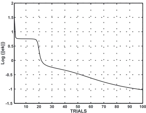
Figure 1: Log_||ek||for a generic system

"learning gain"βk+1to minimize the performance index

J(βk+1) =||ek+1||2+wβ2k+1, w >0 (18)

wherew > 0is introduced to provide a degree of caution in the change in magnitude of the control

signal from iteration to iteration. The results of Owens and Feng can be summarised as follows:

1. The ILC dynamics is described by the iterative matrix equation

ek+1 = (I −βk+1GK)ek, k≥0 (19)

2. The optimal value ofβk+1minimizing the performance index is given by

βk+1 =

eT kGKek

w+_||GKek||2

(20)

where_{|| · ||}is the Euclidean norm.

3. The sequence of learning gains converges to zero ask_{→ ∞}as

X

k≥0

4. The error sequence is monotonically improving in the sense that

||ek+1|| ≤ ||ek|| ∀k≥0 (22)

with equality holding if, and only if,βk+1 = 0.

Note: this is an important benefit of POILC as it provides natural embedded improvement from

iteration to iteration through learning gain changes.

5. The error sequence_{ek}k≥0 converges to a point in theLimit SetS∞defined by the relation

S∞={e: eTGKe= 0 } (23)

Note: In practice the intersection of this set with _{e : _||e_{|| ≤ ||}eo||}is more precise but, for

simplicity, this detail is omitted.

6. The error converges to zero for all initial choices ofu0and hencee0if and only ifG+GT is

strictly sign definite.

7. All points in S∞ are limits of the POLIC algorithm for some choice of e0 (simply choose

e0 ∈S∞.

Sign definiteness ofGK + (GK)T _{is both necessary and sufficient for guaranteed convergence of}

the error to zero. In principle, the condition can be satisfied easily by, for example, the choice of

K=GT _{orK =G}−1 _{but there is obviously a price to be paid in terms of complexity of the control}

computations. The choice of a simpler form ofK may hence be preferred or be desirable for other

reasons. Unfortunately, this condition is then often not satisfied and the consequent price of simplicity

is that convergence to anon-zerolimit errore∞ ∈S∞will occur. A number of issues and questions

can now be stated:

1. The magnitude _||e∞|| of the limit error in both absolute terms and relative to the magnitude

||e0||of the initial error are clear measures of algorithm success.

2. The form ofe∞is also relevant and hence, in particular, information on those regions ofS∞

that attract solutions will be valuable.

3. The dependence and sensitivity of the limit error to the initial errore0 is of interest.

4. The development of algorithms that reduce the impact or eliminate the impact of a limit set

The following sections provide useful insight into the dynamical effects of the existence of a limit set

S∞6={0}and the existence and form of simpleswitching algorithmsthat guarantee convergence of

the error to zero. In these sections, for notational simplicity, we denoteM =GK.

5

Attractivity and Sensitivity Properties of the Limit Set

In this section, limiting properties of iterations of the general form

ek+1= (I−βk+1M)ek, βk+1=β(ek) (24)

where

β(e) = e

T_{M e}

w+_||M e_||2 (25)

are considered withw >0. The associated limit set is defined by

S∞={e:eTM e= 0}={e:β(e) = 0} (26)

which is clearly the set of error time series whereβ = 0. The general objective is to identify more

detailed structural properties that effect algorithm performance. The work extends that in Owens et

al [7] to provide a more complete description including necessary and sufficient conditions.

5.1 Attracting and Repelling Components

Close to the limit set, the fact that β(e) is small indicates that the change in error ek+1 −ek =

−β(ek)M ekis small in magnitude and hence the POILC algorithm is converging slowly. Slow

con-vergence is an undesirable property so it is natural to ask whether or not the limit set isattracting

orrepellingsuch behaviours. Attraction can be interpreted as indicating that the ILC algorithm is

indeed slowing down with little further improvement in error magnitudes possible. Repelling can be

associated with a temporary slowing of the algorithm convergence, more rapid convergence being

regained when the error time series has finally moved away from the limit set.

Whether or not the limit set repels or attracts local time series can be characterized in terms of

sign properties of the sequence_{βk+1}k≥0close toS∞. More precisely:

1. It is easily seen that a pointe_∈S∞attracts trajectories in its vicinity (in the sense that|βk+1|

is getting smaller) if

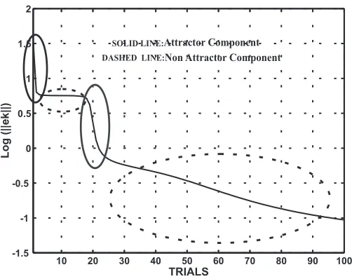
SOLID LINE:Attractor Component Non Attractor Component

DASHED LINE:

Figure 2: Different regions of attraction in theS∞

for all trajectories entering a sufficiently small ball centred on the pointe_∈S∞. This

expres-sion has the simpler form

−2< β_k−₊₁1 (βk+2−βk+1)<0 (28)

Whenβk+1 is small, this expression, together with the expressionek+1 −ek = −βk+1M ek,

can be analysed using the quantity

B(e) = ∂β(ˆe)

∂eˆ |ˆe=eM e (29)

to produce the following sufficient condition for the pointe_∈S∞to attract trajectories toS∞

−2< lim

ek→e

β_k−1∂β(ˆe)

∂ˆe |ˆe=ekβkM ek =−B(e)<0 (30)

2. In a similar manner, if one of the following conditions holds

B(e)>2 , _B(e)<0 (31)

then the pointe_∈S∞repels trajectories.

3. In the cases of_B(e) =₋2or_B(e) = 0the situation is more complicated and is not considered

here.

The quantity_B(e) is clearly central to the behaviour of the algorithm close to S∞ with the point

e_∈S∞attracting trajectories being defined by the relations

The form of_B(e)is therefore important and is computed below:

B(e) = e

T_{(M +M}T_{)M e}

w+_||M e_||2 −β(e)

eT_2MT_M2_e

w+_||M e_||2 (33)

which, whene_∈S∞, is just

B(e) = e

T_{(M +M}T_{)M e}

w+_||M e_||2 (34)

In summary, the following theorem has been proved and extends the results in [7] to provide necessary

and sufficient condition:

Theorem 1 1. A pointe_∈S∞={e:eTM e= 0}attracts local trajectories of ILC algorithm if

it lies in the attracting componentS−

∞⊂S∞defined by the equations

eTM e= 0 , _B(e) = e

T_(M+MT_{)M e}

w+_||M e_||2 ∈(0,2) (35)

2. If, however, it satisfieseT_{M e= 0and one of the inequalities}

B(e)>2 , _B(e)<0 (36)

then it repels local trajectories and is said to lie in the repelling componentS∞+ ⊂S∞.

Note: The cases whereeTM e= 0and_B(e) =₋2or_B(e) =₋2are not considered here. They lie on the boundary between the two sets defining attracting components and repelling components

respectively and will require further analysis to resolve their characteristics.

The condition for the pointeto lie inS−

∞can be rewritten in the form of quadratic inequalities

eTM e= 0 , 0< eT(M +MT)M e <2(w+_||M e_||2) (37) The analysis of this expression as a function of the weightwcan proceed as follows: firstly note that

S−

∞is defined by

eTM e= 0 , eT(M+MT)M e >0 , 0< eT(M ₋MT)M e <2w (38) which reduces in size asw_→0+. Hence:

• Increasingwtherefore tends to increase the size of the attracting componentS−

∞ ⊂ S∞ and

hence increases the potential for convergence to non-zero limit errors.

• For sufficiently large values of w (relative to the range of _||e_|| of interest), the only active

inequality is the simple quadratic inequalityeT_{(M +M}T_{)M e > 0. In particular, for anye}

satisfying this inequality, examination of _B(e) indicates that there exists aw∗

≥ 0 such that

e_∈S−

∞for allw > w∗.

5.2 A 2-D Example

The purpose of this section is to illustrate the ideas using a simple example and reveal sensitivity

properties of ILC algorithms close toS∞+. Consider the case of2-dimensional matrixM:

M =   1 0 α 1 

, M +MT =   2 α α 2   (39)

with eigenvalues ofM+MT _{atλ= 2±αand eigenvectorsv}+_{= (1,1)}T_{, v}−_{= (}

−1,1)T_{.Note that}

(M+MT_{)is sign-indefinite iff α}2 _>4

Solutions ofeT_{(M +M}T_{)e= 0(represented in the orthogonal eigenbasis of(M +M}T_{)), can}

be written in the form:

e=γ

à √

α₋2

  1 1  ± √

α+ 2

  −1 1   ! (40)

whereγ _∈Ris arbitrary.

S∞ 6= {0}wheneverα > 2and can be associated with he two subspacesS+andS−shown in

fig.(3) corresponding to the different values_±of (40). They are strongly connected to the components

S+

∞andS∞− ofS∞. More precisely, evaluating,

eT(MT +M)M e=γ2³2α(α2₋4)_∓2α2pα2₋₄´

it can be verified that it is negative onS+ _{and positive onS}− _{ifα > 2. It follows thatS}+ _{⊂ S}+ ∞

andS−

∞ ⊂ S−. That part of S− that can be identified withS∞− is described by the solutions of

the inequality_B(e) < 2 i.e. eT_{(M −M}T_{)M e < 2w. That this leads to nontrivial solutions can}

be illustrated by looking at the case ofα = 3. In this case, a simple calculation indicates that this

relation is satisfied inS−_{for any choice ofγ}2 _{∈ Randw > 0i.e. S}− _=S−

∞andS+ = S∞+. The

details are omitted for brevity.

The theory indicates (and computation supports) the notion that trajectories originating ate0close

to the attracting component converge to a limit in that component with little decrease in error norm

i.e algorithm performance is very poor. The situation is more complicated close to the repelling

component. Trajectories originating close toS∞+ ultimately converge to limits inS∞− but there is a

surprising sensitivity issue. The above example can also be used to illustrate this sensitivity to the

choice of initial error,e0. More precisely, the behaviour of the error sequence following the initial

errore0close toS∞+ depends critically on "which side ofS∞+ e0lies". To illustrate this, letw= 10−6

and consider the paire0= (1−

√

e

e

S-S+

ë

2

ë

Figure 3: The componentsS−_andS+_ofS ∞

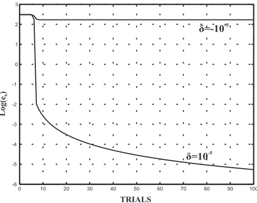
0 10 20 30 40 50 60 70 80 90 100

-6 -5 -4 -3 -2 -1 0 1 2 3

TRIALS Log

(e

)k

ä=-10-5

ä=10-5

Figure 4: Log(_||ek||2)/kwith10−5and−10−5 displacements frome0 ∈S∞−

the point(1₋√5,1 +√5)T _∈S−

∞are applied. In fig.(4) the different in performance of the sequence

of error norms is shown over100iterations. The difference in performance is remarkably large; in

the case of a negative perturbationδ = ₋10−5_{, very little improvement in error norm magnitude is}

achieved whereas, for the case of a positive perturbationδ = 10−5 _{a substantial and rapid decrease}

in magnitude is achieved after10iterations. In both cases, the first10iterations show little change in

norm - a slow variation that is expected close to the limit set.

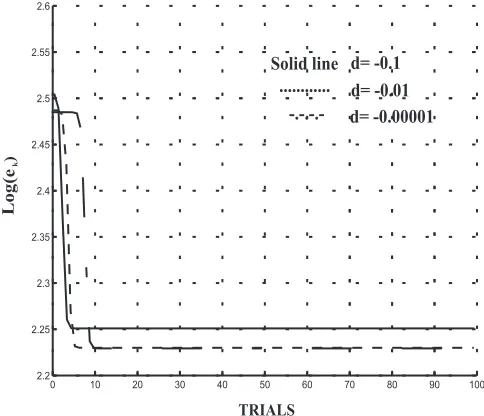
Using the same example, consider the cases whenδ is varied using the positive and increasing

values δ = 10−1_,10−2_,10−5_{. the results are given in fig. (5) with the expected conclusion that,}

the smaller the perturbation, the greater the tendency for the error norm to change slowly and hence

stay close toS+

illustrates the tendency of the error norm sequence_{||ek||}k≥0 to exhibit"stair-like"properties close

toS+

∞i.e a period of slow variation followed by a period of fast convergence followed by another

period of slow convergence.

0 10 20 30 40 50 60 70 80 90 100

2.2 2.25 2.3 2.35 2.4 2.45 2.5 2.55 2.6

TRIALS Log(e

)k

Solid line d= -0.1 d= -0.01 d= -0.00001 ...

-.-.-.-Figure 5: Log(_||ek||2)/kwith different displacements frome0 ∈S∞−

5.3 A Discussion of N-D Possibilities

The2₋Dexample illustrates the potential practical importance of the limit set to the ILC algorithm

(seen as a dynamical system). In particular, the slow convergence close to the limit set may be a

prob-lem and lead to increased iterations (to achieve a required error tolerance) and stair-like behaviours

where slow convergence is seen at least twice during the iteration sequence.

The purpose of this section is to support the intuition that these properties will also be seen in

more complex examples. In this section, theN-dimensional case will be considered in a similar

manner to the2-dimensional example. This is done using a suprisingly simple non-positive plant of

the form;

G(s) = 1

(s+ 1)2 (41)

With sample intervalh= 0.1, a discrete time representation of (41) is obtained:

Φ =





0.81435 ₋0.090484

0.090484 0.99532



, ∆ = 



0.090484

0.0046788





C = (0, 1) (42)

The reference signal was chosen to ber(t) = e20t sintover the time intervalt∈[0,20]. The value

of the weight parameterwisw= 10−6_{and the initial control sequence was as chosen to beu} 0 = 0.

The control matrix was chosen to beK=Ifor simplicity so thatM =G.

The eigenvalues of the resulting200x200matrix(M+MT_{)are in the range of(−0.2086,1.8942),}

so it is not a positive definite matrix i.e. S∞contains non-zero points inR200- a high dimensional

space.

Fig.(6) shows the evolution of the norm of the error and the evolution of the quantity Q =

eT

k(G+GT)Gek

eT

kek . This second quantity is included to illustrate the general correlation between the rate

of convergence and the sign of_B(e). Clearly periods of slow convergence are associated with periods

where_B(e)is positive whilst periods of faster convergence are associated with periods where_B(e)

is negative. One of the remarkable aspects of this example is the fact that stair-like behaviours are

present withthreeperiods of slower convergence and two periods of faster convergence in the first

100iterations. This suggests that stair-like behaviours may be a common feature of parameter optimal

ILC and that they can occur several times within the iteration sequence.

Log(||e

||)_k

e

(G+G

)Ge

/e

e

k

k

k

k

T

T

T

Figure 6: Error dynamics and the sign ofeT

k(G+GT)Gek

In conclusion, the great potential of POILC to produce the very beneficial property of monotonic

ex-istence, in general, of a non-trivial limit set. The existence of this limit set can be associated with

a number of algorithm properties that could reduce performance and, at worst, make the algorithm

effectively impractical. Further work on this issue is desirable but the important question considered

in the following sections is whether or not POILC algorithms can be simply modified to remove some

of the undesirable features. The very positive answer obtained forms the motivation and basis for

further work.

6

Global Stabilisation Using Switching Algorithms

The previous section has indicated that the limit set for a given algorithm introduces serious dynamical

properties into the algorithm. In this section, the issue of generating simple algorithms that ensure

convergence to zero is addressed. No assumption on the nature of the linear systemGis required but

the relative degreek∗_{is assumed known.}

6.1 Switching using Dense Search

To motivate the analysis, note that the limit set is afixedset in_RN+1−k∗ part of which attracts the error sequence_{ek}k≥0. The limit set depends crucially uponM =GKthrough the choice ofK. If

Kis changed, then the limit set will change (at least in part). The natural question to ask if whether

or not variations inK (and hence the Limit Set) from iteration to iteration can ensure convergence

of the tracking error to zerowithout the need for any positivity assumptions. The following analysis

provides a positive answer to this question based on the idea of sweeping through a countably dense

set of suchK. That the variation ofK has the potential to restrict the limit set is indicated by the

following theorem:

Theorem 2 Let_K =_{K₍i,j)}i,j≥1be any countably dense set of matrices whose closure contains a

compact annulus in_R(N+1−k∗)×(N+1−k∗)defined by a relation of the form0< M2_{≤ ||}K_||2 _≤M2. Then

\

K∈K

{e:M =GK, eTM e= 0 _}=_{0_} (43)

Proof: If incorrect, there exists a vector e ₆= 0 such that, also using continuity, eT_{M e = 0 for}

M =GKandK anymatrix. Independent variations of the diagonal elements ofKthen lead to the

conclusion thate= 0which is a contradiction.2

Intuitively, this result is interpreted to suggest that, if a sufficiently rich mechanism is introduced

error norm, the absence of afixedlimit set will perhaps ensure convergence to zero. This truth of this

intuition and its development into a number of conceptual algorithms is the subject of this section.

Suppose that the previous POILC algorithm is replaced by the modified algorithm using the same

performance index but the iteration-dependent control law

uk+1 =uk+βk+1Kk+1ek (44)

As a consequence, the POILC optimal parameter is defined by

βk+1=

eT

kMk+1ek

w+_||Mk+1ek||2

, Mk+1 =GKk+1 (45)

The specification of the algorithm is completed by carefully choosing the sequence of the operations

Kk+1. In what follows the kth choice of Ki,j is specified as the kth element in the (i, j) index

sequence

(1,1),(2,1),(1,2),(1,1),(2,1),(1,2),(3,1),(2,2),(1,3),(1,1),(2,1), .... (46)

obtained using successive sweeping of an increasing triangle of data in the top left hand corner of

the infinite matrix depiction of the elements of_K. The crucial aspect of the sequencing is that every

element of_Kis used and repeatedly used an infinite number of times.

Using optimality, it is easily proved (asukis suboptimal) that

||ek+1||2+wβk2+1 ≤ ||ek||2 (47)

and hence that the monotonicity of the error norm is still guaranteed. Alsoβk+1→0.

From its construction,_Kcontains a pointK =Kp,qsufficiently close toαGT (for someα >0) to

ensure thatGK+(GK)T >0. Consider the subsequence with indices_{kj}j≥0such thatKkj =Kp,q.

Asβk+1 → 0, then eTkjGKp,qekj → 0from whichlimj→∞||ekj|| = 0. Using the monotonicity of

the error norm, the above completes the proof of the following theorem:

Theorem 3 With the above construction, the defined "dense search" switching algorithm guarantees

convergence to zero error for all linear systems of relative degreek∗. Moreover

1. monotonicity of the error norm is guaranteed from iteration to iteration

||ek+1|| ≤ ||ek|| ∀k≥0 (48)

2. the learning gain sequence converges to zero as

X

k≥0

β_k2₊₁<+_∞ (49)

The result underlines the great potential of switching algorithms for POILC as convergence is

guar-anteed for all plants of relative degreek∗ _{on any interval0}

≤ t _≤ N and for any reference signal

time seriesr. Its value is mostly conceptual as dense search is not a particularly practical option. The

following section suggests that finite switching algorithms exist that retain the properties of dense

search.

6.2 Existence of Finite Switching Algorithms

Theorem 4 There exists a (non-unique) finite set _{K˜j}1≤j≤N+1−k∗ that retains the convergence

properties of the POILC dense search algorithm ifKk is selected using the "circulation algorithm"

K(k−1)(N+1−k∗_)+j = ˜Kj for allk≥1and1≤j ≤N+ 1−k∗.

Proof: The proof is by construction. By constructionGis invertible so define

˜

Kj =G−1diag{δi,j+ǫ}1≤i≤N+1−k∗ (50)

whereδi,j is the Kronecker Delta and ǫ > 0. The first part of the proof looks at the intersection

of the solutions of a set of equations each of which will define possible values of cluster points of

subsequences. More precisely, if, for anye_{∈ R}N+1−k∗

,

eTGK˜je=e2j +ǫ

X

i≥0

e2_i = 0, 1_≤j_≤N+ 1₋k∗ (51)

then, for sufficiently smallǫ(e.g 0 <ǫ < _N+11_−k∗), it follows thate= 0.

Turning now to the POILC algorithm, monotonicity of the error norm sequence and convergence

ofβk+1to zero follow in the normal manner from optimality. Monotonicity ensures the existence of

(possibly non-unique) cluster pointse∞i of every subsequence{ej(N+1−k∗_)+i}j≥0,1 ≤ i ≤ N + 1₋k∗_{. Clearly e}

∞i satisfies eT∞iGK˜ie∞i = 0. Next note that the set of all such cluster points

is independent ofias the convergence of theβk+1 to zero proves that, if e∞i is a cluster point of

subsequences with indexi, it is also a cluster point of subsequences with indexi+ 1. All such cluster

points are the simultaneous solutions of the equations defined above and hence, ifǫis sufficiently

small, the only possible cluster point is the limite∞= 0.2

The result indicates that the use ofN + 1₋k∗ _{switching matrices is sufficient for convergence}

convenience and is not unique. The following discussion looks at a number of possibilities that have

simple dynamical systems interpretations.

6.3 Switching Between Causal First Order Filters

The benefits of switching for convergence has been demonstrated above but the methods, as presented,

are relatively complex. Ideally, the switching algorithm should have the desired properties of ensuring

convergence and yet be conceptually simple for implementation e.g. the use of the inverse system

above is not ideal and simpler, more "robust" schemes would be preferred. In what follows, the use

of simple, first order filters is considered using the finite set

˜

Kj =KFj, 1≤j≤Ns, Ns≥N + 1−k∗, (52)

uk+1=uk+Kk+1ek (53)

and the "circulating assumption"

KkNs+j = ˜Kj =KFj, k≥0, 1≤j ≤Ns (54)

HereK is a fixed element (included for generality) and eachFj is selected to be a simple, distinct

dynamical system. In this section it is chosen to be a matrix representation of the transfer function

Fj(z) =

1₋λj

1₋λjz−1

(55)

(normalized such thatFj(1) = 1) which is a simple first order filter with pole at the positionz=λj.

All poles are assumed to be real and distinct and, for practical reasons, in the open interval(₋1,1)to

ensure stability of the filter. The matrix representation is precisely

F(λ) = (1₋λ)

           

1 0 0 . . . 0

λ 1 0 . . . 0

λ2 _{λ 1 . . . 0}

..

. ... ... . .. ...

λN−k∗

λN−k∗₋₁

. . . 1

            (56)

evaluated atλ=λj. For convenience, define the quadratic form

ρ(λ, e) =eTGKF(λ)e(1₋λ)−1 (57) which is also a polynomial inλof degree less than or equal toN ₋k∗_{. The following theorem states}

the convergence properties of the above algorithm which is based on the analysis of limit sets and the

fact thatρis either identically zero or cannot have more thanN₋k∗_{roots and hence cannot haveN}

s

Theorem 5 Suppose thatM =GK has the property that, for allp _≥1, thep_×pPrincipal Minor

ofM generated by rows and columns indexed byN+ 2₋k∗

−p _≤i, j _≤N + 1₋k∗_{is nonzero.}

Then with the above notation, the POILC algorithm

uk+1 =uk+βk+1Kk+1ek, yk+1=Guk+1+d (58)

with

βk+1 = arg min{J(βk+1) =||ek+1||2+wβk2+1}=

eT

kGKk+1ek

w+_||GKk+1ek||2

, w >0, (59)

whereKk+1 circulates through the finite set{KFj}1≤j≤Ns, is convergent to zero error in the sense

that

lim

k→∞ek= 0 & X

k≥0

β_k2₊₁ <_∞ (60) Notes:

1. The assumption on GK is generically satisfied and is satisfied for the following illustrative

cases

• K is a representation of any linear, proper time-invariant dynamical system,

• K is obtained via the inverse algorithmK = G−₀1 whereG0 is a sufficiently good

ap-proximation toGor

• K is chosen to beK =GT

0 whereG0 is a sufficiently good approximation toGT (when

the property of the Principal Minors follows from the fact thatGGT _{is positive definite.)}

2. Note that no other assumption is made on the form of the systemG(orGK) and, in this sense,

the algorithm has universal stabilising properties.

3. For implementation purposes, the matrix computationFjekis best undertaken using the

stan-dard realisation of the transfer functionFj(z).

Proof of the Theorem: The proof follow in a similar way to the previous result i.e monotonicity

follows from the POILC paradigm andβk+1→0in the manner required. Also the intersection of the

sets_{e:ρ(λj, e) = 0},1≤j≤Nsdefines the set of all cluster points of the algorithm. The proof is

complete if it is shown that the only error vectoresatisfying these equations is the single pointe= 0.

Firstly note that it follows that ρ(λ, e) = 0,_∀λ asρ has degree less thanN + 1₋k∗

≤ Ns.

As a consequence, all coefficients ofλj_{,1 ≤ j ≤N + 1−k}∗ _{are zero. It is easily seen that these}

coefficients are given by

whereF is a(N + 1₋k∗₎

×(N + 1₋k∗_{)matrix with elementsδ}

i,j+1i.e.

F =            

0 0 0 . . . 0

1 0 0 . . . 0

0 1 . . . 0

..

. ... ... . .. ...

0 0 . . . 0

           

, FN+1−k∗ = 0 (62)

and henceFℓ_{is a matrix with elementsδ} i,j+ℓ.

For notational convenience, letM have the column structureM = [m1, m2, . . . , mN+1−k∗]with

eachmj ∈ RN+1−k

∗

. With this notation, the vanishing of the coefficients ofρis represented precisely

by the equations

0 =e1eTmN+1−k∗

0 =e2eTmN+1−k∗+e₁eTm_N−k∗

0 =e3eTmN+1−k∗+e₂eTm_N−k∗+e₁eTm_N−1−k∗

.. .

0 =eN+1−k∗eTm_N+1−k∗+e_N−k∗eTm_N−k∗+· · ·+e₁eTm₁

(63)

Ife ₆= 0, then suppose that ej is the first non-zero element. It follows that eTmN+2−k∗−j = 0.

Examination of the structure of the relationships and the use of an inductive argument then yields

eT_m

i = 0, j≤i≤N+ 1−k∗and the assumption on the Principal Minors then indicates thate= 0

which is a contradiction. Hence the only possible limit vector ise= 0. This completes the proof of

the result.2

6.4 Switching Between Non-causal Filters

Similar results can be obtained for non-causal filtering. Although it is not yet known (conclusively)

whether or not causal or no-causal filtering is the best practical option, the following brief discussion

indicates that there is little theoretical difference between the two options in terms of convergence

properties.

Using the notation of previous sections, consider the choice of

˜

Kj =KFjT, 1≤j≤Ns, Ns≥N+ 1−k∗ (64)

AsFT

j =F0FjF0, the computations forFjTekare approached by passing the time reversed errorek

For analysis purposes, the effect of the change ofFj toFjT is to replaceρby

ρ(λ, e) =eTGKFT(λ)e(1₋λ)−1 (65) from which the following theorem follows in a similar manner to the case of causal filters. The proof

is omitted for brevity.

Theorem 6 Suppose thatM =GKhas the property that, for allp_≥1, thep_×pPrincipal Minor of

Mgenerated by rows and columns indexed by1_≤i, j_≤pis nonzero. Then with the above notation,

the POILC algorithm

uk+1 =uk+βk+1Kk+1ek, yk+1=Guk+1+d (66)

with

βk+1 = arg min{J(βk+1) =||ek+1||2+wβk2+1}=

eT

kGKk+1ek

w+_||GKk+1ek||2

, w >0, (67)

whereKk+1circulates through the finite set{KFjT}1≤j≤Ns, is convergent to zero error in the sense

that

lim

k→∞ek= 0 & X

k≥0

β_k2₊₁ <_∞ (68)

6.5 Random Choice of Filters

The result for non-causal filters has exactly the same general form and interpretation as that for the

causal filtering case. The obvious intuition is that there are many more suitable switching mechanisms

with the set of possible finite switching mechanisms being very rich. Further research could identify

improved options to the simple options introduced above. Four features do however seem worthy of

emphasis and may apply more generally:

1. In both cases considered in this paper, the minimum number of filters required isN + 1₋k∗

(although more can be chosen). In general, this is a large number (becauseN is large) and the

likely consequence of choosing fewer is to create a limit set S∞ 6= {0} with the consequent

possibility for convergence to non-zero limit errors.

2. The theory provides no information on the ordering of a given set of filters, yet in practice,

one could expect that the ordering is important to issues such as the rate of convergence. The

3. The choice of distinct poles λj ∈ (−1,1)is arbitrary in the sense that the choice has no

ef-fect on the proof of the results. This leaves open the question of the choice of poles and, in

particular, the effect of any choice on algorithm performance. At this time there seems to be

no theoretical mechanism that could, for example, distinguish between the benefits of equally

spaced distribution of polesλj within the open interval (−1,1)and a more randomly spaced

set of poles on a (possibly much smaller) subinterval [a, b] _⊂ (₋1,1). In both cases, large

values ofNswill tend to make the density large. In this sense, the two cases are the same yet

the spacing over(₋1,1)will introduce a much richer set of filter dynamics as compared to the

case when_|a₋b_{| ≪}1i.e. when all filter poles are close together.

4. Stable filters have been used to reflect practical stability needs. More generally, there is no

theoretical reason to prevent the choice of unstable filters!

As a preliminary practical approach to the resolution of these problems,

1. based on the intuition that a broader range of filter dynamic characteristics will increase the

flexibility of the algorithm, this section assumes that variation of poles over the whole open

interval(₋1,1)is to be preferred.

2. In addition, it is proposed that the large number of poles (Ns) needed and the difficulty in

choosing the positioning and ordering of such poles makes it reasonable to expect that arandom

choice of poles and hence filtersat each iterationwill be an effective practical approach.

3. It is also assumed that the use of standard uniform random number generators to create the

sequence of poles_{λj}j≥0is sufficient to provide the properties sought.

The concept has practical appeal. However, the theoretical difficulty with the concept is that it is not

covered by the previous theorems. Its performance is, as a consequence, unknown. However, given

the fact that, for each iteration of POILC, monotonicity of the norm is guaranteed plus the observation

that random search is conceptually related to dense search in that all intervals of all sizes in the search

space are visited an infinite number of times, convergence is expected on intuitive grounds.

7

A Numerical Study

The purpose of this section is to illustrate the possible performance of the switching algorithms

pro-posed. Results are provided for the case using random, causal filters only. The simple algorithm

for exploration is that examined in section 5.3. where the potentially poor convergence properties of

the basic POILC method were illustrated. The poor convergence can be seen in Fig.(6) where the

reduction of the logarithmic norm (squared) of the error from5.7 to only5.2over100iterations is

seen.

In what follows, it will be seen that the use of switching algorithms based on causal filters and the

choice of a sequence of stable filter poles uniformly distributed in(₋1,1)has the potential to greatly

improve algorithm performance. Being random, the approach has no guarantees but, statistically,

substantial benefits could be expected on average. Important insight into these statistical benefits

is provided below for the given example through computational experiments using repeated runs of

POILC from the same starting condition but using differing (uncorrelated) random pole sequences in

each run. This is presented below with the conclusion that the most probable outcome in practice is a

substantial improvement on the non-switching case.

The sequence of calculations undertaken was as follows:

1. 100iterations from the initial controlu0 = 0were undertaken using a pseudo random number

generator to create a sequence of uniformly distributed poles _{λk}k≥0 in the open interval (₋1,1). The experiment was repeated a number of times using different independent sequences

but starting at the same starting point (i.e. the input to the first iterationu0 = 0). The generated

sequences of logarithmic squared error norms is given in fig.(7).

2. The results show the wide range of performance made possible (over100iterations) by the use

of random switching. The improvement in error norm squared observed ranges from around

three to five orders of magnitude (compared to the non-switching case) although the earlier

rate of convergence varies more widely as is seen at 40 iterations where performance ranges

from little improvement to three orders of magnitude. It is interesting to note that individual

norm sequences consist of periods of modest reduction with sudden substantial improvements

although these cannot be predicted theoretically.

3. A more detailed analysis of the statistical behaviour of the approach was obtained by repeating

the algorithm (from the same initial error) for350independent random sequences_{λk+1}k≥0

uniformly distributed in(₋1,1). These are illustrated using a frequency diagram in histogram

form to identify the frequency with which the results generated logarithmic norms at iteration

Log(||e

||)

2

Figure 7:Log(_||ek||2)vkfor several independent sequences of random filters

-0.5

-0.5 0.00.0 0.50.5 1.01.0 1.51.5 2.02.0 2.52.5 3.03.0 3.53.5 4.04.0 00

3 55 8 10 10 13 15 15 18 20 20 23 25 25 28 30 30 33 35 35 38

Final value of Log(||e

||

)

NumberofAppearances

-0.8 -0.5-0.5 -0.3 0.00.0 0.3 0.50.5 0.8 1.01.0 1.3 1.51.5 1.8 2.02.0 2.3 2.52.5 2.8 3.03.0 3.3 3.53.5 3.8 4.04.0 0

20 40 60 80 100 120 140

NumberofAppearances

Final value of Log(||e

||

)

Figure 9: Frequency ofLog(_||e100||2)for1450independent random choices of filter sequences

frequency distribution has a simple statistical form with the most probable outcome at iteration

100improving the initial squared error norm_||e0||2by a factor of around106i.e. an

improve-ment of in_||e0||of a factor of103.

4. Finally, the form of frequency distribution obtained above was refined by repeating the

cal-culation again over 100iterations but for the increased number of1450independent random

sequences uniformly distributed in (₋1,1). The results are shown in fig.(9) and reaffirm the

conclusions reached above. Increasing the number of random sequences further supports these

conclusions but details are omitted for brevity.

The conclusion reached from this example is that the use of randomly chosen filters in simple

param-eter optimal ILC is an effective tool in overcoming the problems of temporary and asymptotic poor

convergence due to non-trivial stable components of the limit set. For the example chosen (where

little error norm reduction is obtained without switching), the most probable benefits of switching

(over100iterations) indicate improvements in norm reduction of several orders of magnitude. These

benefits are expected more generally and are not specific to the system chosen or the choice of100

iterations. A surprising observation is that these improvements are obtained over100iterations which

8

Conclusions

The use of Parameter Optimal Iterative Learning Control has the benefit of ensuring monotonic

con-vergence of the Euclidean norm (mean square value) of the error time series but will tend to produce

non-zero limit errors lying within a well-defined but high-dimensionallimit setS∞⊂RN+1−k ∗

. The

form of the limit set is critically dependent on the choice of algorithm and the form of plant

dynam-ics. This phenomenon can lead to very poor improvements in performance and a number of other

problems. These issues can be, in part, described by the properties of the attractingS−

∞and repelling

componentsS+

∞ofS∞. Both components lead to slow convergence when the error trajectory is close

to them. In addition there are potential sensitivity properties closeS∞+ and a tendency to generate

stair-like behaviourswhere apparent convergence is, in fact, temporary slow convergence close to

S∞+ which is ultimately replaced by a period of faster convergence. This can happen several times

over many iterations leading to difficulties in practice in deciding when to terminate the algorithm.

An understanding of the limit set has successfully suggested that the use of switching algorithms

can remove many of these problems and, in theory, provide an attractiveguarantee of convergence to

zero error independent of plant dynamics i.e., in a theoretical sense, switching algorithms are globally

successful. The possible choices of switching sequence seems to be very rich. Dense search can be

used but, in general it is sufficient to use "only"N + 1₋k∗_{switching values. The use of causal and}

non-causal first-order filters (with distinct poles) has been shown to be a simple and effective way

forward. This still leaves a large choice of switching elements and there remains problems of the

choice of, for example, filter poles and the order in which they are to be used. Numerical computation

based on the random choice of switching filters has demonstrated that a statistical approach has great

potential. Computational examples show that it can considerably improve convergence properties

with the "most-probable" error reduction being orders of magnitude better than that obtained in the

non-switching case.

Although the paper has provided substantial theoretical support for the ideas introduced, there are

many issues that arise from the developments. These include the development of a more rigorous

general approach to the statistical method proposed (a difficult problem as the POILC method is

nonlinear in the filter poles). Of particular value here would be the characterization of the frequency

distribution function of the logarithmic error norm at a specified iteration. The simple form observed

in the frequency plots computed in this paper suggest that these distributions could have quite simple

forms. A simpler (but not necessarily simple) objective might be to compute the Expectation of_||eℓ||

This paper has not answered all relevant questions. Amongst the many issues that arise is the

ultimate need to consider the robustness with respect to resetting of the initial condition and plant

modelling error. These are non-trivial deterministic and stochastic questions that are left for future

research and publications to resolve.

9

Final Comments

The second author was responsible for the computational results. The work described in this paper is

covered by pending patent applications in the UK and elsewhere.

References

[1] Arimoto, S., Kawamura, S. & Miyazaki, F. Bettering operations and robot learning,Journal of

robotic systems, vol. 1, 1984, pp 123-140.

[2] Moore, K.,Iterative learning control for deterministic systems, Springer, London; 1993.

[3] Moore, K. & Xu, J-K.Special Issue of the international Journal of control on Iterative Learning

Control, 73(10); 2000.

[4] Owens, D.H. & Feng, K.Parameter Optimization in Iterative Learning Control, Internatioanl

Journal of Control, vol 76(11), 1059-1069, 2003.

[5] Hatönen, J.J., Owens, D.H., Feng,K. Basis Functions and Parameter Optimization in

High-Order Iterative Learning Control, Automatica, vol. 42, Issue 2, 287-294 , 2006.

[6] Owens, D.H. & Hatönen, J.J.Iterative Learning Control - an Optimization Paradigm, IFAC

Annual Reviews in Control, vol. 29, Issue 1, 57-70 , 2005.

[7] Owens, D.H., Maria Tomas-Rodriguez & Hatönen, J.J.Limiting Bahaviour in Parameter