This is a repository copy of
Sources of error in road safety scheme evaluation: a method
to deal with outdated accident prediction models.
.
White Rose Research Online URL for this paper:
http://eprints.whiterose.ac.uk/2462/
Article:
Hirst, W.M., Mountain, L.J. and Maher, M.J. (2004) Sources of error in road safety scheme
evaluation: a method to deal with outdated accident prediction models. Accident Analysis &
Prevention, 36 (5). pp. 717-727.
https://doi.org/10.1016/j.aap.2003.05.005
[email protected] https://eprints.whiterose.ac.uk/ Reuse
See Attached
Takedown
If you consider content in White Rose Research Online to be in breach of UK law, please notify us by
Universities of Leeds, Sheffield and York
http://eprints.whiterose.ac.uk/
Institute of Transport Studies
University of Leeds
This is an uncorrected proof version of a paper published in Accident Analysis &
Prevention. It has been uploaded with the permission of the publisher. It has
been refereed but does not include the publisher’s final corrections.
White Rose Repository URL for this paper:
http://eprints.whiterose.ac.uk/2462
Published paper
Hirst W.M, Mountain L.J. and Maher M.J. (2004) Sources of error in road safety
scheme evaluation: a method to deal with outdated accident prediction models.
Accident Analysis and Prevention 36(5), 717-727.
UNCORRECTED PROOF
Accident Analysis and Prevention xxx (2003) xxx–xxx
Sources of error in road safety scheme evaluation: a method to
3
deal with outdated accident prediction models
4
W.M. Hirst
a, L.J. Mountain
a,∗, M.J. Maher
b5
aDepartment of Civil Engineering, University of Liverpool, Brownlow Street, Liverpool L69 3GQ, UK
6
bSchool of the Built Environment, Napier University, Edinburgh, UK
7
Received 14 May 2003; accepted 23 May 2003
8
9
Abstract
10
This paper considers the errors that arise in using outdated accident prediction models in road safety scheme evaluation. Methods to correct for regression-to-mean (RTM) effects in scheme evaluation normally rely on the use of accident prediction models. However, because accident risk tends to decline over time, such models tend to become outdated and the estimated treatment effect is then exaggerated. A new correction procedure is described which can effectively eliminate such errors.
11 12 13 14
© 2003 Published by Elsevier Ltd. 15
Keywords: Road safety; Regression-to-mean; Trend in risk; Correction for bias
16 17
1. Introduction 18
The task of estimating the effect of a road safety scheme
19
on the mean frequency of accidents is not straightforward.
20
While observations of accidents before and after treatment
21
can establish the change in mean accident frequency, it is
22
unlikely that all of the observed change can be attributed
23
to the effects of the scheme. The primary task in scheme
24
evaluation is then that of separating scheme effects, S, from
25
the changes that would have occurred without the scheme, N.
26
In a recent paper (Hirst et al., in press) the authors considered
27
in detail the various factors that can have a confounding
28
effect in the evaluation of road safety schemes and suggested
29
a simple additive model to describe these.
30
The three main non-scheme sources of change in
ob-31
served accident frequencies are regression-to-mean (RTM)
32
effects; trends in accidents; and local changes in flow (due
33
to transport or land use changes unrelated to the scheme
un-34
der study). The observed change in annual accidents, B, can
35
be written as
36
B=S+N
37
The non-scheme effects are then
38
N =NT+NF+NR
39
∗Corresponding author. Tel.:+44-151-794-5226;
fax:+44-151-794-5218.
E-mail address: [email protected] (L.J. Mountain).
where NT is the change due to national trends in accidents 40
over the period of observation arising as a result of the com- 41
bined effect of trends in risk and in flow; NF the change in 42
accidents due to local changes in flow other than those at- 43
tributable to trend but unrelated to the study scheme and NR 44
is the change in accidents due to the RTM effect. 45
The change in accidents attributable to the scheme may 46
be in part due to the effect of the scheme on accident risk 47
(accidents per unit of exposure), SR, and in part due to the 48
effect of the scheme on flow, SF. Thus 49
S=SR+SF 50
and 51
B=SR+SF+NT+NR+NF 52
The authors (Hirst et al., in press) have proposed a mod- 53
ification to current methods which allows the reduction in 54
accidents attributable to each of the five causal factors to be 55
separately evaluated. The proposed approach, in common 56
with others that include a correction for RTM effects (see, 57
for example,Hauer, 1997; Elvik, 1997), relies on the avail- 58
ability of suitable predictive accident models. These are as- 59
sumed to represent the relationship between mean accident 60
frequency and various explanatory variables (typically traf- 61
fic flow and site characteristics) during the scheme evalua- 62
tion period. The problem is that, in practice, this assumption 63
will rarely be satisfied because of the effects of trends in 64
accidents. 65
1 0001-4575/$ – see front matter © 2003 Published by Elsevier Ltd.
2 doi:10.1016/j.aap.2003.05.005
UNCORRECTED PROOF
2. Outdated accident prediction models 66
To appreciate the problem, it is useful to briefly consider
67
the nature of the evaluation process. In order to estimate
68
the true scheme effect, it is necessary to estimate what the
69
expected accident frequency in the period after treatment
70
would have been had the scheme not been implemented. A
71
common approach is to use an empirical Bayes (EB) method
72
(see, for example, Maher and Summersgill, 1996; Hauer, 73
1997; Elvik, 1997). In this the mean accident frequency
74
in the before period is estimated as a weighted average of
75
observed accidents before treatment, XB, and a predictive
76
model estimate of expected accidents given the nature of
77
the site and the level of traffic flow. The general form of
78
predictive accident models is
79
ˆ
µ=CqβB
80
where C is a constant for each site (incorporating the
rele-81
vant site characteristics for the particular model used), qBa
82
measure of traffic flow in the period before treatment andβ
83
is the predictive model coefficient for flow. The predictive
84
model estimate of total accidents in a before period of tB
85
years is then
86
ˆ
µB=tBµˆ
87
Generally such predictive models assume that the random
88
errors are from the negative binomial (NB) family. If K is
89
the shape parameter for the NB distribution, the EB estimate
90
of total accidents in the before period,MˆB, is calculated as
91
ˆ
MB=αµˆB+(1−α)XB
92
where
93
α=
1+µˆB
K −1
94
The EB estimate of expected accidents in the after period in
95
the absence of the scheme,MˆA, can then be estimated. The
96
effects of general trends in risk and flow on accidents during
97
the study period can be accounted for by using a comparison
98
group ratio of accidents
99
AA NAT
AB NAT
100
where AB NATis the total national (or regional) accidents in
101
the before period of tByears and AA NATis the total national
102
(or regional) accidents in the after period of tAyears.
103
The use of a comparison group ratio implicitly assumes
104
that flows at the study site have changed in line with national
105
or regional trends. To take account of the effects of any
106
local flow changes, while avoiding double counting, it is
107
necessary to have a representative measure of traffic flow
108
at the scheme in the after period, qA, together with flow
109
data for the comparison group. If QB NAT: total national (or
110
regional) flow in the before period, QA NAT: total national
111
(or regional) flow in the after period, then the expected flow 112
in the after period if flows at the study site had changed in 113
line with general trends,q′A, can be estimated using 114
q′A=
QA NAT/tA
QB NAT/tB
qB 115
If the observed flow in after period, qA, differs from q′A 116
then there have been local changes in flow at the site other 117
than those attributable to trend. If, on the basis of local 118
knowledge, these are judged to be due to transport or land 119
use changes unrelated to the scheme under study, then the 120
expected accidents in the after period in the absence of the 121
scheme is 122
ˆ
MA= ˆMB A
A NAT
AB NAT
qA
q′A β
123
If, on the other hand, the local flow changes are judged to 124
be a consequence of the scheme itself, then 125
ˆ
MA= ˆMB A
A NAT
AB NAT
126
If XA accidents are observed at the scheme site in the after 127
period, the scheme effect is estimated as 128
ˆ
S=(XA/tA)−(MˆA/tA)
XB/tB 129
and the non-scheme effects as 130
ˆ
N= (MˆA/tB)−(XB/tB)
XB/tB 131
It is clear that the EB approach implicitly assumes that the 132
predictive model represents the relationship between acci- 133
dents and flows in the before period at the study site. Equally, 134
the comparison group approach implicitly recognises that 135
there can be an underlying trend in risk within the study pe- 136
riod. However, no allowance is made for the effects of trend 137
in risk between the time period used for modelling and the 138
time period used for scheme assessment: this in spite of the 139
fact that available models are typically derived using histor- 140
ical data, often for a period of time many years prior to the 141
study period used for scheme assessment. 142
The standard form of the available predictive models as- 143
sumes that the risk of accidents, C, per unit of exposure, 144
qβ, is constant over time. The value of C represents the av- 145
erage risk per unit of exposure during the modelled period. 146
In practice we do not expect accident risk per unit of expo- 147
sure (C) to remain constant over time: the whole purpose of 148
many road safety initiatives is to reduce risk at a regional or 149
national level. Measures such as improvements in road user 150
training, national road safety awareness initiatives, and speed 151
enforcement campaigns are all believed to reduce accident 152
risk per unit of exposure. In the UK there is evidence to sug- 153
gest that accident risk as a function of exposure has been 154
declining over time. For example, for the years 1975–1995, 155
UNCORRECTED PROOF
W.M. Hirst et al. / Accident Analysis and Prevention xxx (2003) xxx–xxx 3
based on national data, the average rate of decline in
acci-156
dent risk was found to be 2% per year while for a subset of
157
roads in six English counties over the period 1980–1991 the
158
rate of decline was estimated to be 5% per year on link
sec-159
tions and 6% per year at major junctions (Mountain et al., 160
1997, 1998). It has recently become recommended practice
161
in the UK (DfT, 2002) to allow for trends in accident risk,
162
with the predicted annual change depending on the location.
163
For most urban roads (speed limit≤40 mph) the predicted
164
decrease in risk is 1.6% per year, with a decrease of 0.09%
165
at major urban junctions and 2.4% at minor junctions.
166
If it is accepted that there are trends in risk over time then
167
it must also be recognised that predictive models that do not
168
allow for trend in risk will rapidly become outdated: they
169
represent the average accident risk per unit of exposure only
170
over the modelled period. As a consequence, if the before
171
period for the scheme to be evaluated is not contained within
172
the modelled period, the estimates of accidents in the before
173
period will be biased. Since predictive models are generally
174
based on historical data, the elapsed time between the
mod-175
elled period and the before period (and hence the effects of
176
trend) may well be large. For example, a typical model for
177
UK urban single carriageway roads was derived using
ac-178
cident data for a 5-year-period from April 1983 to March
179
1988 (Summersgill and Layfield, 1996). The models
rou-180
tinely used to predict accidents at UK intersections (Binning, 181
1996, 2000) are based on accident data for the 6-year-period
182
1974–1979 in the case of four-arm roundabouts and for the
183
period 1984–1989 in the case of urban priority intersections.
184
While it would, of course, be theoretically possible to
up-185
date predictive accident models at regular intervals, this is
186
not normally done in practice because of the high cost of
187
carrying out such studies.
188
A more appropriate form of predictive model would be
189
one which allows for trend in risk. One such model (Maher 190
and Summersgill, 1996) takes the form
191
ˆ
µt =C0γtqβt 192
whereµˆt is the expected number of accidents in year t; C0
193
the risk in year 0;γ the factor by which risk changes from
194
year to year and qt is the flow in year t. 195
This model is a marginal model that avoids modelling
196
the year-to-year variation but allows for trend in risk based
197
on an annual change factor (γ). The merits of various trend
198
models are discussed by Lord and Persaud (2000)but this
199
form of model is perhaps the most fruitful to consider here
200
since the change in risk from year to year is fixed, allowing
201
predictions beyond the modelled period.
202
While models which allow for trend have been fitted
203
to accident data (Mountain et al., 1997, 1998; Lord and 204
Persaud, 2000) such models are not widely available: for
205
most site types in most regions the only available predictive
206
accident models do not include a trend term. This is in part
207
because suitable data are not readily available: ideally
acci-208
dent and traffic counts for many years are needed, with the
209
traffic counts for each year treated as separate observations. 210
In addition, the disaggregation of the data presents diffi- 211
culties for traditional model fitting procedures (Maher and 212 Summersgill, 1996,Lord and Persaud, 2000). The aim in 213
this study was therefore to produce a correction for the bias 214
introduced by using the more commonly available form of 215
model: an outdated accident prediction model with no trend 216
term. 217
3. Bias arising from using the model without trend 218
The underlying assumption is that the trend model out- 219
lined above is the correct form of model. If a predictive 220
accident model of the formµˆt =Cqβt is fitted when there 221
is actually a trend in risk, the model is mis-specified. It is 222
necessary to consider what implications this may have for 223
estimates of expected accidents. 224
It is assumed, for a sample of sites, that accident and 225
flow data are available for each year of an n year modelling 226
period. Accidents will have a mean ofµ0 = C0q0β in the 227
first year of the study period (t =0) and in the final year 228
(t=n−1) a mean ofµ(n−1)=C0γ(n−1)qβ(n−1). The model 229
without trend is normally derived using a single estimate of 230
the mean observed flow in the model period,q¯, and thus, for 231
the total n-year-period, the fitted model is 232
Cq¯βn∼NB
n−1
t=0
µi, K
, where
n−1
t=0
µi=C0
n−1
t=0
γtqβt
233
A simple rearrangement of the model equation and the total 234
true accident mean gives 235
C= C0
n−1
t=0γtq
β t ¯
qβn =
mean accidents
(mean flow)β 236
Thus C could be estimated as a function of mean accidents 237
and flows. It can be assumed that the mean of accidents and 238
the mean of flows occur at approximately the middle of the 239
modelled period (at timet =(n−1)/2). This is illustrated 240
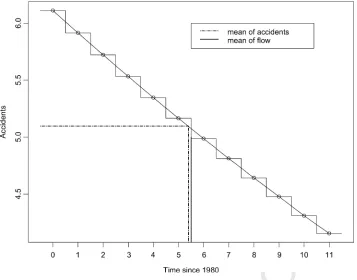
for a specific example inFig. 1. In line with the results of 241 Mountain et al. (1997), the example is for a 12-year modelled 242
period (1980–1991) for a site with typical flows withC0= 243
3,β=0.61 andγ =0.95. It can be seen that the mean of 244
accidents and of flows both occur close to the mid-point of 245
the modelled period (t=5.5 in this example). 246
In practice, the mean flow will only occur at the mid-point 247
of the modelled period if flows follow an arithmetic progres- 248
sion but this assumption should not be unreasonable if flows 249
are not changing too dramatically over time. The assump- 250
tion that the mean of accidents occurs in the middle year is 251
also not likely to be strictly true since it is assumed that the 252
decline in risk follows a geometric progression while flows 253
are increasing: again if flows are not changing too dramati- 254
cally over time, andγis reasonably close to 1, this assump- 255
tion should not be unreasonable. Under these assumptions, 256
UNCORRECTED PROOF
Fig. 1. Accidents for 1980–1991 (typical UK link flow withC0=3,γ=0.95 andβ=0.61).
it is possible to equate the models at the middle of the
mod-257
elling period (t=(n−1)/2). If it is also assumed that the
258
power of flow (β) is the same for both models (not
neces-259
sarily true since available models have a range of values for
260
βand estimates ofβ and C are not independent) then
261
C≈ C0γ
(n−1)/2q¯β
¯
qβ =C0γ (n−1)/2
262
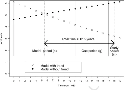
Assuming thatC=C0γ(n−1)/2,Fig. 2shows how the
pre-263
dicted before mean accident frequency (µˆB) for a study site
264
some years after the modelled period would be affected by
265
trend in risk. In this hypothetical example, the scheme site
266
has a before period of 3 years (1997–1999) and the
mod-267
elled period is 12 years (1980–1991) as before. There is
268
thus a gap of 5 years (1992–1996) between the end of the
269
modelled period and the start of the before period. Traffic
270
flows are assumed to increase arithmetically over time (in
271
line with the actual growth in traffic flow in the UK over the
272
period 1980–1999). Thus the model without a trend in risk
273
term shows an increase in expected accidents in each year,
274
in line with the increase in flow. The model with a trend
275
term reflects the combined effects of the increasing traffic
276
flows together with the declining accident risk (γ =0.95).
277
The overall effect in this case is a decrease in expected
ac-278
cidents over time.
279
The two models, under these assumptions, are equivalent
280
at the mid-point of the modelled period. Assuming that, for
281
the 3-year before period at the scheme, the mean of flows
282
also occurs in the middle year, the effects of trend between
283
the middle of the modelled period and the middle of the 284
before period can be estimated. For this it is convenient to 285
shift the time datum point (t = 0) to the middle of the 286
modelling period. With this time datum, att=0,µ0=Cqβ0 287
and for subsequent yearsµt =Cγtqβt. The last year of the 288
modelled period occurs att=5.5 (i.e.t =(n−1)/2), the 289
last year of the gap between the end of the modelled period 290
and the start of the before period will be att =10.5 (i.e. 291
t=((n−1)/2)+g, where g is the duration of the gap). The 292
middle of the before period will occur in the second year of 293
the 3-year-period att = 12.5. More generally, if tB is the 294
duration of the before period as before, 295
t=
n−1
2
+g+
t B+1
2
=g+
n+t B
2
296
For this example, the estimated means (µˆBorµtˆ B) obtained 297
using the models with and without trend would differ by a 298
factor ofγ12.5(the trend model giving the smaller estimate). 299
This result leads to the possibility of a correction 300
procedure which could be applied to any mis-specified 301
model. Thus, more generally, if µˆB is estimated using a 302
mis-specified predictive model which makes no allowance 303
for trend, the estimate (µˆB NO TREND) can be corrected using 304
ˆ
µB CORRECTED=γtµˆB NO TREND 305
whereγis the factor by which risk changes from year to year 306
and t the elapsed time between the middle of the modelling 307
and study periods=g+(n+tB)/2. 308
UNCORRECTED PROOF
[image:7.595.100.503.69.358.2]W.M. Hirst et al. / Accident Analysis and Prevention xxx (2003) xxx–xxx 5
Fig. 2. Accidents for 1980–1999 (typical UK link flow withC0=3,γ=0.95 andβ=0.61).
This definition of the expected bias arising when fitting
309
a model without a trend in risk term to data which exhibits
310
trend relies on a number of assumptions. No attempt has
311
been made to mathematically derive these suggested results
312
and instead justification is now sought via simulation.
313
4. Simulation studies to determine the magnitude 314
of bias 315
Simulations were carried out to assess the relationships
316
suggested above. The aim in the simulations was to reflect
317
the conditions that might be encountered in a typical
acci-318
dent study. It was thus necessary to select typical time
peri-319
ods; typical accident model parameters; and typical accident
320
trends. It was also necessary to generate observed accident
321
data for typical safety scheme study sites: sites which are
322
normally selected (at least partially) on the basis of a high
323
accident frequency in a particular time period and thus
sub-324
ject to a RTM effect in a subsequent time period.
325
Each simulation study followed a pre-defined time
pe-326
riod. This comprised a modelling period of either 5 years
327
or 12 years ending in 1991, a gap of 3 years between the
328
end of the modelling period and the study period, and a
329
7-year study period for new sites under investigation. The
330
5-year modelling period is typical of the periods used to
de-331
rive models with no trend term; the 12-year-period was that
332
used byMountain et al. (1997)to derive a model with trend.
333
The 7-year study period comprised a 3-year before period
334
(1995–1997), a 1-year investigation and treatment period, 335
and a 3-year after period (1999–2001). The underlying pop- 336
ulation characteristics for the trend model (C0,β,γand K) 337
were fixed in advance. The true parameters were chosen so 338
thatC0=3 (reflecting an average value for treated sites cur- 339
rently under investigation in a research project at the Uni- 340
versity of Liverpool), withβ=0.61 andK=1.92 (in line 341
with the Mountain et al. (1997)model for link data). The 342
annual change in risk was set at 2.5 and 5% (γ=0.975 and 343
0.95): in line with the UK national trend in risk over the pe- 344
riod 1980–2001 (3%) and with theMountain et al. (1997, 345 1998)model for link data for 1980–1991 (5%). The number 346
of sites (nmod) in the sample used to estimate the model 347
parameters was also fixed at 100 (chosen to represent a typ- 348
ically sized data set such as that used bySummersgill and 349 Layfield (1996)) and at 1000 (roughly the size of the data set 350
used byMountain et al. (1997)to fit trend models for link 351
data). The different combinations of time period, number of 352
sites and values ofγmeant that eight individual simulation 353
studies were carried out. 354
Each simulation consisted of 500 realisations. For each of 355
the 500 realisations, nmod sites were generated from the true 356
underlying population characteristics C0,β,γ and K. Each 357
of the nmod sites followed a randomly generated subset of 358
the model period. 359
In order to calculate the mean accidents at each site it was 360
necessary to simulate traffic counts. This was done so that 361
overall flows followed an arithmetic progression (the best 362
fitting model to UK national flow data for the hypothetical 363
UNCORRECTED PROOF
study period) and so that the overall total flows for the nmod
364
sites increase by a factor of 1.9 from 1975 to 2000 (again in
365
line with UK national flow data), although annual flows at
366
individual sites could vary from this relationship from year to
367
year. The distribution of flows across sites was generated to
368
reflect the observed flows used by Layfield and Summersgill
369
(1996) to derive a model for urban single carriageway roads.
370
Once a flow vector for each of the nmod sites had been
371
generated, the true underlying mean accidents for that site
372
was known. This, together with the NB shape parameter K,
373
was used to generate observed accidents at the site from a
374
NB distribution.
375
The models with and without a trend term were then
fit-376
ted to the observed data for the nmod sites, giving estimates
377 ˆ
C0,βˆTRENDandγˆ for the trend model andCˆ andβˆNO TREND
378
for the model without trend. Estimation for the trend model
379
was achieved via the algorithm outlined by Maher and 380
Summersgill (1996). This is an approximate fit based on
381
linearising the predictors using constructed variables (see,
382
for example,Atkinson, 1985; Cook and Weisberg, 1982).
383
For each of the eight simulations (consisting of 500 model
384
realisations), 100 study sites were generated following an
385
overall average (but not individually fixed) observed change
386
in accidents of either−50% or−75%. Observed accidents
387
in the before period were generated from the true mean,
388
µTRUE for each study site. An unknown, but definite RTM
389
effect was achieved by rejecting any generated before period
390
accidents less than twice the true mean and re-sampling (i.e.
391
sites withXB<2µTRUE rejected, as might typically be the
392
case in selecting candidate sites for safety schemes).
393
For both the correctly specified trend model and the
394
mis-specified model without trend, the bias in the estimate
395
of the true mean was defined asτ, where
396
τµTRUE= ˆµB
397
For the model without trend
398
τ =µˆB NO TREND
µTRUE
= tB
ˆ
Cq¯βˆNO TREND
C0t∈BEFORE PERIODγtq
β t 399
For the model with trend
400
τ =µˆB TREND
µTRUE
= ˆ
C0t∈BEFORE PERIODγˆtq
ˆ
βTREND
t
C0t∈BEFORE PERIODγtq
β t 401
For the trend model (if the parameter estimates are
un-402
biased) it would be expected that the mean of τ would
403
be 1 while, for the model without trend (for a study
pe-404
riod after the modelled period), it would be expected that
405
τ >1. The main reason for examining any bias resulting
406
from a correctly specified trend model was to examine
407
the stability of the approximation in estimating the model
408
parameters.
409
It is important to examine the biases that may arise, not
410
only in the predictive model estimates (µˆB), but also in the
411
EB estimates (MˆB). This is used to estimateMˆA and hence
412
the scheme and non-scheme effects (SR, SF, NT, NRand NF) 413
(Hirst et al., in press). The bias in the EB estimate is 414415
ρ= MˆB
MB TRUE
=(KTRUE+µTRUE)(Kˆ +XB)µˆB
(Kˆ + ˆµB)(KTRUE+XB)µTRUE 416
= (KTRUE+µTRUE)(Kˆ +XB)
((K/τ)ˆ +µTRUE)(KTRUE+XB) 417
ifKˆ ≈KTRUE then 418
ρ≈ (KTRUE+µTRUE)
((K/τ)ˆ +µTRUE) 419
The bias in the EB estimates for individual sites, and in the 420
estimates of the effects of regression-to-mean (NR), trend 421
(NT) and treatment effects (SR and SF) were examined for 422
each of the 500 studies of 100 sites. (It was assumed in this 423
study thatNF=0.) 424
5. Results from the simulation studies 425
The simulation studies demonstrated that the relationship 426
between C0and C was consistent with that suggested (C≈ 427
C0γ(n−1)/2) and the estimate of β from both models was 428
unbiased. The bias in the predictive model estimate of mean 429
accidents in the before period was thus also consistent with 430
that suggested previously. Thus 431
E(τ)=γ−t, wheret=g+
n+t B
2
432
A simple correction to the estimate from the model without 433
trend is therefore to multiply the estimated before mean from 434
the mis-specified model by the inverse of the expected bias 435
ˆ
µB CORRECTED= ˆµB NO TREND(E(τ)−1) 436
which is equivalent to the correction procedure proposed, 437
namely 438
ˆ
µB CORRECTED=γtµˆB NO TREND 439
Clearly this correction requires an estimate of γ. If total 440
annual flows (QNATi) and accidents (ANATi) are available 441
for an appropriate comparison group over the relevant time 442
period, then an estimate ofγ can be obtained by fitting a 443
model of the form 444
ANATi=A0γiQNATi fori=0, . . . , ((n−1)+g+st) 445 Table 1 summarises the bias in the predictive model esti- 446
mates of mean accidents in the before period (µˆB) and the 447
bias in the EB estimates (MˆB) obtained using the three ap- 448
proaches: the trend model, the mis-specified model without 449
trend and the proposed correction procedure. Using a data 450
set of 1000 sites and a modelling period of 12 years, the 451
estimates obtained using the trend model were as expected, 452
with the mean and median of the bias (τTREND) close to 1. 453
UNCORRECTED PROOF
W.M.
Hir
st
et
al.
/Accident
Analysis
and
Pr
evention
xxx
(2003)
xxx–xxx
7
Table 1
Bias in the predictive model estimates of mean accidents in the before period (τ) and the EB estimates (ρ)
γ, model period (years), n
τTREND τNO TREND τCORRECTED ρTREND ρNO TREND ρCORRECTED
Mean Median S.D. Mean Median S.D. Mean Median S.D. Mean Median S.D. Mean Median S.D. Mean Median S.D.
0.95, 5, 100 3.97 1.07 11.6 1.44 1.43 0.16 1 1 0.11 0.92 1.01 0.27 1.05 1.04 0.03 1 1 0.03 0.95, 5, 1000 1.14 1.01 0.58 1.43 1.43 0.05 1 1 0.03 0.99 1 0.08 1.05 1.04 0.03 1 1 0.01 0.95, 12, 100 1.16 0.98 0.70 1.72 1.71 0.19 1 1 0.11 0.97 0.99 0.14 1.09 1.07 0.05 0.99 1 0.03 0.95, 12, 1000 1.02 1.01 0.18 1.72 1.72 0.06 1 1 0.03 1 1 0.04 1.09 1.07 0.05 1 1 0.01 0.975, 5, 100 3.31 0.93 7.9 1.2 1.19 0.13 1 1 0.11 0.9 0.99 0.26 1.02 1.01 0.03 1 1 0.03 0.975, 5, 1000 1.14 1.02 0.59 1.2 1.19 0.04 1 1 0.04 0.99 1 0.07 1.02 1.02 0.01 1 1 0.01 0.975, 12, 100 1.18 1.01 0.79 1.31 1.3 0.15 1 1 0.11 0.98 1 0.11 1.03 1.03 0.03 0.99 1 0.03 0.975, 12, 1000 1.02 1 0.17 1.3 1.3 0.04 1 1 0.03 1 1 0.03 1.04 1.03 0.02 1 1 0.01
Mean: mean of bias; med: median of bias; S.D.: standard deviation of the bias. Results are shown to two decimal places.τTREND: bias in predictive model estimates using trend model;τNO TREND: bias
in predictive model estimates using model without trend;τCORRECTED: bias in predictive model estimates using correction procedure;ρTREND: bias in EB estimates using trend model;ρNO TREND: bias in
EB estimates using model without trend;ρCORRECTED: bias in EB estimates using correction procedure.
AAP
1003
UNCORRECTED PROOF
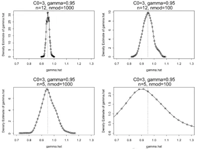
Fig. 3. Density of 500 estimates ofγfor four cases in the simulation study (whereC0=3,β=0.61 andγ=0.95). The dashed lines represent the true
value ofγ=0.95.
However, the algorithm for fitting the trend model proved
454
inefficient using a data set of only 100 sites or a modelling
455
period of only 5 years: the distribution of bias was skew,
456
with the mean bias tending to be much greater than 1. This
457
is illustrated in Fig. 3. It can be seen that, withn=5 and
458
nmod=100, in the extremes of the distribution the before
459
mean can be greatly under- or over-estimated. This result
460
would suggest that the successful fitting of a trend model of
461
the type used here requires data for a large number of sites
462
over many years.
463
As expected, the bias in the model without trend
464
(τNO TREND) is substantial, particularly whenγis
apprecia-465
bly less than 1 and n (and hence t) is large. For the case of
466
γ=0.95 andn=12 (t=10.5), the mean over-estimate of
467 ˆ
µBusing the model without trend was 72%. The correction
468
procedure proved extremely effective in estimating the
be-469
fore mean: both the mean and median ofτCORRECTED are
470
1 for all cases.
471
The results for the distribution of bias in the EB
esti-472
mates (Table 1) show that, using the model without trend,
473
the before mean (MˆB) was consistently over-estimated
474
(ρNO TREND > 1) although the bias was much closer to 1
475
than that in the estimates of µˆB (τNO TREND). In the most
476
extreme case, withγ =0.95 andn=12, the model
with-477
out trend over-estimated MˆB by 9%. Although the model
478
with trend (τTREND) performed well when the model period
479
was 12 years, the trend models derived from 5 years data
480
for 100 sites introduced more bias than the model without 481
trend. For example, in the case of γ =0.95 (with n = 5 482
and nmod = 100), the model with trend led to a mean 483
under-estimate of MˆB of 8% (τTREND = 0.92) compared 484
with a mean over-estimate of 5% using the model without 485
trend (τNO TREND =1.05). Again the correction procedure 486
proved extremely effective in estimating the before mean 487
(MˆB), withτCORRECTED≈1 in all cases. 488
The distribution of estimates of scheme and non-scheme 489
effects for studies of nmod =1000 are shown in Table 2 490
for γ = 0.95 and Table 3for γ = 0.975. The use of the 491
model without trend tended to result in under-estimates of 492
regression-to-mean effects (NR) and over-estimates of treat- 493
ment effects (SR+SF), although the bias is not particularly 494
large. The correction procedure was successful in eliminat- 495
ing bias in all cases: even when the underlying trend in 496
risk was large, the correction consistently estimated the true 497
treatment effect. 498
6. Application of correction method to real data 499
The uncorrected and corrected models without trend were 500
also applied to a group of 50 real sites at which a variety of 501
speed management measures had been applied. Total per- 502
sonal injury accidents and fatal and serious accidents were 503
analysed. All of the sites were in 30 mph speed limits and 504
UNCORRECTED PROOF
W.M.
Hir
st
et
al.
/Accident
Analysis
and
Pr
evention
xxx
(2003)
xxx–xxx
9
Table 2
The distribution of estimates of scheme and non-scheme effects for studies of nmod=1000 withγ=0.95
Properties Model type B= −0.5 B= −0.75
NR NT SF SR NR NT SF SR
Model time=5 years, size of model data set=1000
True data −0.07{−0.07}[0] −0.13{−0.13}[0] −0.03{−0.03}[0] −0.26{−0.26}[0.04] −0.07{−0.07}[0] −0.13{−0.13}[0] −0.03{−0.03}[0] −0.51{−0.51}[0.02] Trend model −0.08{−0.07}[0.05] −0.13{−0.13}[0.01] −0.03{−0.03}[0] −0.25{−0.26}[0.06] −0.08{−0.07}[0.05] −0.13{−0.13}[0.01] −0.03{−0.03}[0] −0.5{−0.51}[0.05] Without trend −0.04{−0.04}[0] −0.14{−0.14}[0] −0.03{−0.03}[0] −0.29{−0.29}[0.04] −0.04{−0.04}[0] −0.14{−0.14}[0] −0.03{−0.03}[0] −0.54{−0.54}[0.02] Corrected model −0.07{−0.07}[0.01] −0.13{−0.13}[0] −0.03{−0.03}[0] −0.26{−0.26}[0.04] −0.07{−0.07}[0.01] −0.13{−0.13}[0] −0.03{−0.03}[0] −0.51{−0.51}[0.02] Model time=12 years,
size of model data set=1000
True data −0.1{−0.1}[0] −0.13{−0.13}[0] −0.03{−0.03}[0] −0.24{−0.24}[0.04] −0.1{−0.1}[0] −0.13{−0.13}[0] −0.03{−0.03}[0] −0.49{−0.49}[0.03] Trend model −0.1{−0.1}[0.03] −0.13{−0.13}[0] −0.03{−0.03}[0] −0.23{−0.24}[0.05] −0.1{−0.1}[0.03] −0.13{−0.13}[0] −0.03{−0.03}[0] −0.49{−0.49}[0.03] Without trend −0.04{−0.04}[0] −0.14{−0.14}[0] −0.03{−0.03}[0] −0.29{−0.29}[0.04] −0.04{−0.04}[0] −0.14{−0.14}[0] −0.03{−0.03}[0] −0.54{−0.54}[0.03] Corrected model −0.1{−0.1}[0.01] −0.13{−0.13}[0] −0.03{−0.03}[0] −0.24{−0.24}[0.04] −0.1{−0.1}[0.01] −0.13{−0.13}[0] −0.03{−0.03}[0] −0.49{−0.49}[0.03] Cells contain the arithmetic mean,{median}and [standard deviation] of the distribution of each estimate to two decimal places. B: observed proportional change in annual accidents; NR: RTM effect; NT: trend in accidents within study period; SF: scheme effect attributable to a change in flow; SR: scheme effect attributable to a change in risk.
AAP
1003
UNCORRECTED PROOF
W.M.
Hir
st
et
al.
/Accident
Analysis
and
Pr
evention
xxx
(2003)
xxx–xxx
Table 3
The distribution of estimates of scheme and non-scheme effects for studies of nmod=1000 withγ=0.975
Properties Model type B= −0.5 B= −0.75
NR NT SF SR NR NT SF SR
Model time=5 years, size of model data set=1000
True data −0.08{−0.08}[0] −0.05{−0.05}[0] −0.03{−0.03}[0] −0.33{−0.34}[0.05] −0.08{−0.08}[0] −0.05{−0.05}[0] −0.03{−0.04}[0] −0.58{−0.59}[0.03] Trend model −0.09{−0.08}[0.05] −0.05{−0.05}[0] −0.03{−0.03}[0] −0.33{−0.33}[0.07] −0.09{−0.08}[0.05] −0.05{−0.05}[0] −0.03{−0.03}[0] −0.58{−0.58}[0.05] Without trend −0.07{−0.07}[0] −0.05{−0.05}[0] −0.04{−0.04}[0] −0.35{−0.35}[0.05] −0.07{−0.07}[0] −0.05{−0.05}[0] −0.04{−0.04}[0] −0.6{−0.6}[0.03] Corrected model −0.08{−0.08}[0.01] −0.05{−0.05}[0] −0.03{−0.03}[0] −0.33{−0.34}[0.05] −0.08{−0.08}[0.01] −0.05{−0.05}[0] −0.03{−0.03}[0] −0.58{−0.58}[0.03] Model time=12 years,
size of model data set=1000
True data −0.1{−0.1}[0] −0.05{−0.05}[0] −0.03{−0.03}[0] −0.33{−0.33}[0.05] −0.1{−0.1}[0] −0.05{−0.05}[0] −0.03{−0.03}[0] −0.57{−0.57}[0.03] Trend model −0.1{−0.1}[0.02] −0.05{−0.05}[0] −0.03{−0.03}[0] −0.32{−0.33}[0.05] −0.1{−0.1}[0.02] −0.05{−0.05}[0] −0.03{−0.03}[0] −0.57{−0.57}[0.03] Without trend −0.07{−0.07}[0] −0.05{−0.05}[0] −0.04{−0.04}[0] −0.35{−0.35}[0.05] −0.07{−0.07}[0.01] −0.05{−0.05}[0] −0.04{−0.04}[0] −0.59{−0.59}[0.03] Corrected model −0.1{−0.1}[0.01] −0.05{−0.05}[0] −0.03{−0.03}[0] −0.33{−0.33}[0.05] −0.1{−0.1}[0.01] −0.05{−0.05}[0] −0.03{−0.03}[0] −0.57{−0.57}[0.03] Cells contain the arithmetic mean,{median}and [standard deviation] of the distribution of each estimate to two decimal places. B: observed proportional change in annual accidents; NR: RTM effect; NT: trend in accidents within study period; SF: scheme effect attributable to a change in flow; SR: scheme effect attributable to a change in risk.
AAP
1003
UNCORRECTED PROOF
W.M. Hirst et al. / Accident Analysis and Prevention xxx (2003) xxx–xxx 11
the schemes included both speed cameras and a variety of
505
traffic calming measures. There were a total of 733 personal
506
injury accidents in the before period, with 434 in the after
507
period, and the mean durations of the before and after periods
508
were 2.98 and 2.75 years, respectively. There were 131 fatal
509
and serious accidents in the before period with 67 in the
510
after period. The mean of the before period for the 50 sites
511
occurred in September 1997.
512
The predictive accident models used were the models
513
without trend presented by Mountain et al. (1997) with a
514
modelling period of 12 years (1980–1991). Hence the mean
515
time difference from the mid-point of the modelling period
516
to the mid-point of the before periods was roughly 12 years.
517
Correcting for the effects of trend in risk from the model
pe-518
riod to the study period was therefore desirable. The estimate
519
of γused in the correction procedure was obtained from a
520
comparison group consisting of UK accidents and flows for
521
the years 1980–2001: the entire study period for modelled
522
sites and scheme sites. This gaveγ=0.97 for all accidents
523
and γ = 0.94 for fatal and serious accidents.
Calcula-524
tion of traditional confidence intervals for the scheme and
525
non-scheme effects was achieved by the bootstrap (Efron 526
and Tibshirani, 1993). This is a Monte-Carlo technique
527
where samples (of the same size as the original sample) are
528
taken from the data with replacement and the statistic of
529
interest (say SR) is calculated for each sample. The
distribu-530
tion of the estimates from (say 1000 samples) is then used to
531
calculate the standard error of the estimate and the 2.5th and
532
97.5th percentiles give an empirical 95% confidence
inter-533
val. The results for the 50 sites are summarised inTable 4.
534
As was predicted by the simulation studies, ignoring
535
the effects of trend in risk between the modelling
[image:13.595.46.549.475.718.2]pe-536
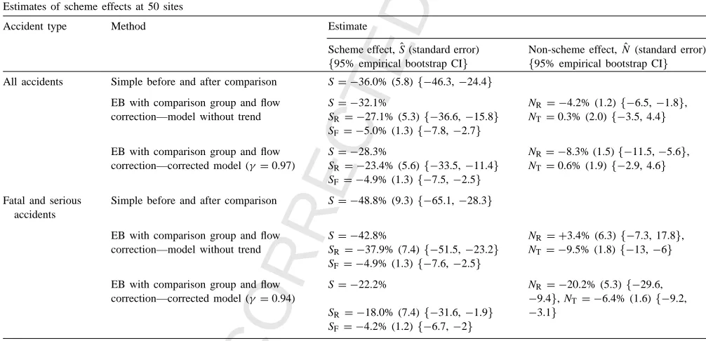
Table 4
Estimates of scheme effects at 50 sites
Accident type Method Estimate
Scheme effect,Sˆ (standard error)
{95% empirical bootstrap CI}
Non-scheme effect,Nˆ (standard error)
{95% empirical bootstrap CI}
All accidents Simple before and after comparison S= −36.0% (5.8){−46.3,−24.4}
EB with comparison group and flow correction—model without trend
S= −32.1% NR= −4.2% (1.2){−6.5,−1.8},
NT =0.3% (2.0){−3.5, 4.4}
SR= −27.1% (5.3){−36.6,−15.8}
SF= −5.0% (1.3){−7.8,−2.7}
EB with comparison group and flow correction—corrected model (γ =0.97)
S= −28.3% NR= −8.3% (1.5){−11.5,−5.6},
NT =0.6% (1.9){−2.9, 4.6}
SR= −23.4% (5.6){−33.5,−11.4}
SF= −4.9% (1.3){−7.5,−2.5}
Fatal and serious accidents
Simple before and after comparison S= −48.8% (9.3){−65.1,−28.3}
EB with comparison group and flow correction—model without trend
S= −42.8% NR= +3.4% (6.3){−7.3, 17.8},
NT = −9.5% (1.8){−13,−6}
SR= −37.9% (7.4){−51.5,−23.2}
SF= −4.9% (1.3){−7.6,−2.5}
EB with comparison group and flow correction—corrected model (γ =0.94)
S= −22.2% NR= −20.2% (5.3){−29.6,
−9.4}, NT = −6.4% (1.6){−9.2,
−3.1}
SR= −18.0% (7.4){−31.6,−1.9}
SF= −4.2% (1.2){−6.7,−2}
S: scheme effect; SR: scheme effect attributable to a change in risk; SF: scheme effect attributable to a change in flow; NT: trend in accidents within
study period; NR: RTM effect.
riod and the study period leads to under-estimates of the 537
regression-to-mean effect (NR), with over-estimates of the 538
scheme effects (S). The impact of the correction procedure 539
was particularly important for fatal and serious accidents: 540
the estimated effect of treatment on fatal and serious acci- 541
dents using the correction (−22%) is only half that obtained 542
assuming a constant risk (−43%). The estimates of the 543
regression-to-mean effect with and without the correction 544
were −20.2 and +3.42% respectively. This is a rather 545
greater impact than might have been anticipated from the 546
simulation results. The simulations, however, were based 547
on a representative value of C0for total accidents. As fatal 548
and serious accidents represent only a proportion of all ac- 549
cidents, the value of C0for fatal and serious accidents will 550
be smaller than for total accidents (with correspondingly 551
smaller values of µˆB and XB). The models presented by 552 Mountain et al. (1997)also give an estimate of the negative 553
binomial shape parameter (K) of 2.65 for fatal and serious 554
accidents compared with 1.92 for total accidents. These 555
factors will clearly affect the EB estimation process and 556
may indicate that for fatal and serious accidents the need 557
for the correction procedure is greater. Further simulation 558
studies (with C0 = 0.75, i.e. only a quarter of the value 559
used in the original simulation studies) have indeed shown 560
this to be true. 561
7. Discussion 562
The majority of available models assume that the un- 563
derlying risk of accidents per unit of exposure is constant 564
over time and yet, if road safety programmes are effective,
UNCORRECTED PROOF
a decline in risk per unit of exposure would be expected.
565
The results of simulation studies show that trend in risk
566
can lead to substantial errors in predictive model estimates
567
of mean accident frequencies if the period for which
esti-568
mates are required is several years after the modelling
pe-569
riod (as is typically the case). The simulation studies also
570
show that, if there is a trend in accident risk, the use of a
571
model which ignores trend will result in errors in estimates
572
of both the regression-to-mean effect and the treatment
ef-573
fect. The size of these errors will depend on the size of the
574
factor by which risk changes from year to year (γ) and on
575
the elapsed time between the mid-points of modelling
pe-576
riod and the study period (t). The errors also tend to be
577
larger for sub-groups of accidents (such as fatal and
seri-578
ous accidents) for which the observed and predicted
acci-579
dent frequencies are smaller, and the NB shape parameter is
580
larger.
581
Given a reliable estimate of the factor by which risk
582
changes from year to year (γ), the correction procedure
out-583
lined in this paper allows an appropriate adjustment for trend
584
in risk to be made to any accident prediction model. Indeed,
585
for models derived from data for a relatively small number
586
of sites over a short time period (say 100 sites over 5 years),
587
it could be preferable to use the correction procedure rather
588
than attempting to fit a model incorporating a trend term:
589
the simulations show that it is not possible to reliably fit a
590
trend model of the type considered here to such data. Since
591
the majority of existing models are derived from data for
592
relatively small number of sites over short time periods, this
593
is an important result.
594
Clearly the quality of the estimates obtained using the
595
correction for trend will rely on the quality of the estimate
596
ofγ. The trend models presented byMountain et al. (1997) 597
for the period of 1980–1991 for link accidents estimateγas
598
0.95 and 0.98 for total accidents and fatal and serious
ac-599
cidents, respectively. This was based on data for 1268 sites
600
and hence the simulations presented here suggest these
esti-601
mates should be stable. There is clearly a discrepancy,
how-602
ever, between these estimates and those obtained using
na-603
tional data for the period 1980–2001 which gave estimates
604
ofγof 0.97 and 0.94 for all accidents and fatal and serious
605
accidents, respectively (and which were used in the
correc-606
tion for the 50 real sites). Discrepancies between the trend
607
estimates for individual links and the national data could be
608
due to various factors: the national data may not be
repre-609
sentative of link sites (the accident totals include all
acci-610
dents not just those on links); the sample of link sites used
611
byMountain et al. (1997)may not be representative of
na-612
tional trends (the data were for only six of the English
coun-613
ties); the factor by which risk changes from year to year (γ)
614
may not be constant over time. There is a need for this to
615
be addressed in future research.
616
In the simulation studies presented in this paper, overall
617
mean flows were assumed to follow an arithmetic
progres-618
sion. This was a strong assumption as it meant the mean of
619
flows occurred at the middle of the study period. Some
fur-620
ther investigations involving other possible representations 621
of flow (such as a geometric progression or a sigmoid curve 622
for flows over the study period) have shown that the correc- 623
tion is still valid. 624
It is perhaps also worth noting that if the true value ofγ 625
is close to 1 (i.e. trend in accident risk is negligible) then 626
observed trends in accidents will be entirely attributable to 627
trend in flow. In this case it could be preferable to estimate 628
expected accidents in the after period using the actual before 629
and after flows at the study site rather than observed acci- 630
dents for a comparison group in the before and after periods 631
(which might not be truly representative of the site under 632
investigation). However, if the true value ofγ is close to 1 633
it would raise questions about the effectiveness of current 634
road safety strategies. 635
8. Conclusions 636
This paper has considered the problems of bias when us- 637
ing a mis-specified predictive model in the estimation of 638
confounding factors in before and after studies of road safety 639
schemes. Under the assumption of a genuine change in risk 640
over time simulations showed that, if this is ignored, the es- 641
timation of RTM and treatment effects can be biased. How- 642
ever, the nature of the bias in the predictive model was es- 643
tablished and a simple correction procedure outlined. The 644
correction procedure was effective in eliminating bias and 645
was also shown to be easily applicable to real data in an 646
analysis of 50 treated sites. 647
Acknowledgements 648
The authors gratefully acknowledge the financial sup- 649
port of EPSRC and the assistance of the staff of the local 650
authorities, their consultants, and the police forces that sup- 651
plied data for this project. The areas for which data have 652
been provided include: Blackpool, Bournemouth, Bradford, 653
Bridgend, Buckinghamshire, Cambridgeshire, Cleveland, 654
Devon, Doncaster, Durham, Essex, Gloucestershire, Here- 655
fordshire, Lancashire, Leicestershire, Lincolnshire, Liver- 656
pool, Norfolk, Northamptonshire, North Yorkshire, Notting- 657
hamshire, Oxfordshire, Poole, Rotherham, Sheffield, South 658
Tyneside, Strathclyde, Suffolk, Swansea, Thames Valley, 659
Wakefield, and Worcestershire. 660
References 661
Atkinson, A.C., 1985. Plots, Transformations, and Regression: An Intro- 662
duction to Graphical Methods of Diagnostic Regression Analysis. 663
Oxford Statistical Science Series. Clarendon Press, Oxford. 664
Binning, J.C., 1996. Visual PICADY/4 User Guide. Transport Research 665
Laboratory, Crowthorne, Berkshire, UK. 666
Binning, J.C., 2000. ARCADY 5 (UK) User Guide. Transport Research 667
Laboratory, Crowthorne, Berkshire, UK. 668
UNCORRECTED PROOF
W.M. Hirst et al. / Accident Analysis and Prevention xxx (2003) xxx–xxx 13
Cook, R.D., Weisberg, S., 1982. Residuals and Influence in Regression.
669
Monographs on Statistics and Applied Probability. Chapman and Hall,
670
New York.
671
Department for Transport, 2002. Design Manual Roads and Bridges, vol.
672
13, Section 1, Part 2. Department for Transport, London.
673
Efron, B., Tibshirani, R., 1993. An Introduction to the Bootstrap. Chapman
674
and Hall, New York.
675
Elvik, R., 1997. Effects on accidents of automatic speed enforcement in
676
Norway. Transport. Res. Record 1595, 14–19.
677
Hauer, E., 1997. Observational before-after studies in road safety. In:
678
Estimating the Effect of Highway and Traffic Engineering Measures
679
on Road Safety. Pergamon Press, Oxford.
680
Hirst, W.M., Mountain, L.J., Maher, M.J. Sources of error in safety scheme
681
evaluation: a quantified comparison of current methods. Accid. Anal.
682
Prev., in press.
683
Lord, D., Persaud, B.N., 2000. Accident prediction models with trend
684
and without trend: application of the general estimating equation
(GEE) procedure. In: Proceedings of the 79th Annual Meeting of the 685
Transportation Research Board, Paper No. 00-0496. Washington, DC, 686
January 2000. 687
Maher, M.J., Summersgill, I., 1996. A comprehensive methodology for 688
the fitting of predictive accident models. Accid. Anal. Prev. 28 (3), 689
281–296. 690
Mountain, L.J., Maher, M.J., Fawaz, B., 1997. The effects of trend over 691
time on accident model predictions. In: Proceedings of the PTRC 25th 692
European Transport Forum, P419, pp. 145–158. 693
Mountain, L.J., Maher, M.J., Fawaz, B., 1998. The influence of trend on 694
estimates of accidents at junctions. Accid. Anal. Prev. 30 (5), 641– 695
649. 696
Summersgill, I., Layfield, R.E., 1996. Non-Junction Accidents on Urban 697
Single Carriageway Roads. TRL Report 183. Transport Research 698
Laboratory, Crowthorne, Berkshire, UK. 699