Application of Vector Control to Permanent Magnet Synchronous Motors Using Chaos Control

Article

Application of Vector Control to Permanent Magnet

Synchronous Motors Using Chaos Control

Elham Hezare

1,a

_{, Mohammad Ataei}

2,b

_,

_{and Mehrdad Jafarboland}

3,c

1 Department of Electrical Engineering, Najafabad Branch, Islamic Azad University, Najafabad

85141-43131, Iran

2 Department of Electrical Engineering, Faculty of Engineering, University of Isfahan, Hezar-jeribst.,

Isfahan 8174673441, Iran

3 Department of Electrical Engineering, Malek Ashtar University of Technology, Shahin Shahr, Isfahan,

Iran

E-mail: a_{[email protected] (Corresponding author),} b_{[email protected],} c_{[email protected]}

Abstract. This paper presents the idea of vector control for permanent magnet synchronous motor (PMSM) based on chaos theorem, using chaos controller. PMSM will demonstrate chaotic phenomena when its parameters fall into a certain area. To achieve this aim, the sub-system of controller has been designed by considering block diagram structure of vector control for PMSM and by applying the setting of Lyapunov exponents method. Also, asymptotical stability of closed loop system with given controller is shown, using the direct Lyapunov method. The performance of designed controller in chaotic mode is compared with conventional vector control methods. Also, the normal mode for PMSM is considered and the performance of controller is compared. Simulation results indicate that not only does this controller eliminate the chaos in chaotic mode and have good performance but also is able to control the system in normal mode by using almost the smaller control signal effort.

Keywords: Vector control, chaos, Lyapunov exponents, permanent magnet synchronous motor.

ENGINEERING JOURNAL Volume 18 Issue 2

Received 21 April 2013 Accepted 8 August 2013 Published 18 April 2014

1.

Introduction

DC motors drives used in the field of variable speed drive until mid-1970s. DC drives was more controllable than AC drives. But Dc drives have some disadvantages such as lack of robustness, overload capability, narrow speed range, and frequent maintenance requirements, particularly due to brushes and commutators. For many years DC motors was used in the modern drive system. Recent developments in microprocessors, magnetic materials, and semiconductor technology have proposed a superior idea to use ac motors in high performance drive (HPD) systems. One of the most popular type of ac motor is the permanent magnet synchronous motor (PMSM) that extensively used in industrial applications because of its simple structure, high efficiency, high power density, and low manufacturing cost[1-2]. High performance drive systems need to accuracy and fast responses, quick recovery of speed from any disturbances and insensitivity to parameter variations because of using them in robotics, rolling mills, machine tools, etc. In these applications, if the closed loop vector control scheme is employed for PMSM, equivalent performance characteristics of a separately excited dc motor can be obtained [3]. With using vector control theory, the dynamic behavior of an ac motor can be obviously improved because speed and torque can be controlled separately.

With using vector control theory in the PMSM drive system, not only the torque and flux components of stator current are decoupled which provides faster response but also makes the control task easy [4]. Proportional integral (PI) or proportional integral derivative (PID) has been widely used in conventional controllers. But if we don’t have an accurate system model, there is more difficulty to design the controller. Moreover, uncertainties and other factors such as noise, temperature, saturation, etc., affect the performance of these controllers for wide range of speed operations [5]. Also, some investigations showed that when systemic parameters falling into a certain area, the PMSM is experiencing chaotic behavior [6-9]. Intermittent ripples of torque and low-frequency oscillations of rotational speed is the backwash of chaos phenomena in PMSM which can extremely destroy the stabilization of the motor, even induce drive system collapse. PI or PID controllers don’t have good performance in this condition. Thus, it is indispensable to study the method of controlling or suppressing chaos in PMSM.

Up to now, there are large numbers of control methods for chaos. Some of them use chaotic system’s behavior for controlling chaos like Ott-Grebogi-Yorke (OGY) and Time Delay Feedback (TDFC) methods, while others are classical methods like linear, nonlinear, adaptive and Fuzzy controllers, which are conventional methods in control theory[10-12]. The most popular method for controlling the chaos in motor systems is OGY [13]. The method is robust in theory but a critical drawback is lack of adjustable parameter in PMSM, so we can’t use this method for PMSM. Zhang et al. [14] suggested the entrainment and migration control strategy to control chaos in PMSM. However, this method does not allow the control objective to be any part of the trajectory of the controlled system and the control law cannot be affected until the states of the system enter into the domain of attractions, which may not be consistent with the requirement of the application. So, practically this method is not desirable. In time-delay feedback control (TDFC) method [15], the direct axis and the quadrature axis stator voltages are used as manipulated variables without an exogenous force. In practice, it is difficult to estimate time delay for TDFC with a given target. More recently, nonlinear feedback control method overcomes the disadvantages of TDFC method [16].

2.

Vector Control of PMSM

The control scheme of PMSM is relative simple. The proposed scheme is presented in Fig. 1.

Fig. 1. Vector control scheme [20].

In this structure voltage source inverter is used to control the feeding currents [21]. The basic idea of vector control is as follows: decomposing the PMSM stator current isinto two components field current component id and its vertical torque current component iq, through the coordinate transformation.iq is equivalent of armature current in DC machine. So, the control scheme is similar to cascaded DC motor control. The PI speed controller provides the reference value for the torque-exciting current iq. Due to the permanent magnets at the rotor, the reference value for the field exciting current id is kept to zero to have maximum torque per ampere. We assume that motor operates in constant torque region and does not require the field weakening.

3.

Chaos in PMSM

The dynamics of a smooth-air-gap PMSM can be modeled based on the d-qaxis [22]:













-

-- -

-p r q L r

r

q s q r d r r

q

d s d r q

d

n i T

D

dt j

u R i Li

di

dt L

u R i Li

di

dt L

 

 



 _

 

 



 _

 

 _

 

 

(1)

where r , iq , and id are the state variables, which denotes motor angular frequency (rad/s) and

quadrature-axis and direct-axis currents (A), respectively;uqandudare the quadrature-axis and direct-axis

stator voltage components (V), respectively; tis the time (s), T_Ldenotes the load torque (N.m), L is the

winding stator inductance (H), Rs stands for the stator winding resistance (Ω), r is the permanent

magnet flux (Wb), β is the viscous damping coefficient (N/rad/s), j is the polar moment of inertia (kg.m2_),

[image:3.595.72.525.126.375.2]

For investigation the chaos phenomena in the PMSM, we must change the variables and normalize them. Assume that τ= L/R, t = t /τ and k=β/( n τΨp r). The normalized state variables ω, iq and id are

defined as follows:

, q ,

d

d q

i i

i i

k k  

   (2)

The dimensionless mathematical model of PMSM is given by





q L

q

q d q

d

d q d

d

i T

dt di

i i u

dt di

i i u

dt

  

 



 _{  }

 

 _{    }

  

   

 

(3)

where   r/kL;   / j;

2 _/

L L

T  T j; u_qu_q/kR_s; ud ud /kRs.

In Eq (3),

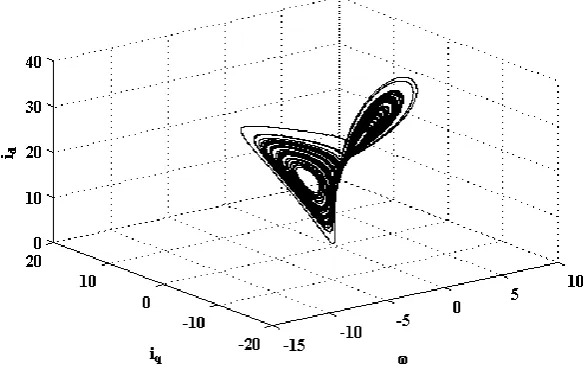
id , iq and ω denote scaled direct-axis current, scaled quadrature current and scaled motor angle speed, respectively; σ and γ are the system parameters. In the practical model of the PMSM, the system parameters σ and γ have uncertainties. By using the modern nonlinear theory such as bifurcation and chaos, the nonlinear dynamical behaviors of system (1) have been studied accurately. The results of investigation have shown that with the systemic parameters σ and γ falling into a specific area, the PMSM endures chaotic behavior. For σ=5.46, γ=30, the PMSM will exhibit chaos. The typical chaotic attractor is shown in Fig. 2.

Fig. 2. Typical chaotic attractor (σ = 5.46, γ = 30).

4.

Controller Design

For designing the controller, we first give a lemma as follows [22]:

Lemma: consider the continuous system (4):

 

x f x u (4)

In system (4) for setting the Lyapunov exponents in the desired value, we use the following control law:

*

ol

u J x

 _{   }

 (5)

*

 = diag ( * 1

 , *

2

 , … , *

n

 ) n n

R

 is an orthogonal matrix where *

i

 is desired Lyapunov exponent and Jol

[image:4.595.152.446.390.574.2]

Remark: The control law (5) is designed for a specific class of systems where _u_Rn_{. If we have}





1

1 2 1

T n

n

u u u u_ R  , the control law is generalized in special conditions. First, we must arrange

the dynamic equations as follows:













1

1 1 2

2

2 1 2 1

1 2 1

, , , , , , , , , n n n

n n n

dx

f x x x

dt dx

f x x x u

dt

dx

f x x x u

dt                 (6)

and if we have 1 1

0, f x

 _

 then control law is generalized, and when putting it into the system (4),

automatically renders the Lyapunov exponent in the first row negative. In this condition the Lyapunov exponent cannot be set in arbitrary value, and control law transforms into the following equation:

2 2 * 1 2 * 1 0 0 n

n n n

n f f x x u x f f x x       _{    }    _{   }       _{   }            (7)

For PMSM, open loop Jacobian matrix is:

0

( ) 1

1 ol d q J i i           _    _  _    (8)

and we have   0, so with respect to (6) and (7) we can control the chaos with setting the Lyapunov

exponent in the desired value. Control inputs are derived as follows [19]:

*

*

q q d q q

d d q d d

u i i i

u i i i

                (9) * q

 and *

d

 are set arbitrary negative Lyapunov exponents. Here, the aim is to eliminate the chaos and not to track desired speed*_{. To this end, stator currents must be regulated. Based on vector control theory, a}

speed feedback loop and a current feedback loop are considered. According to this control technique, instead of using PI controllers, tracking objectives designed using nonlinear control theory in the mechanical sub-system of the PMSM drive. Therefore the reference currents of the PMSM motor is developed to meet necessary torque (or speed) requirements. Subsequent control voltages of the PMSM drive is then derived to force actual current to follow reference values; thus effectively meeting motion control objective which is embedded inside current tracking objectives. Assuming that i_q* and i*_d are the time

invariant constant values, the control law is modified as follows:





* *

* *

( )

q q d q q q

d d q d d d

u i i i i

u i i i i

                  (10)

where * 2 q q P P     (11)









* * * * ( ) q L q

q q q

d

d d d

d i T dt di i i dt di i i dt       _{  }    _{ }        (12)

According to (12) after the controller (10) is put into effect, system (3) has a unique equilibrium ( *

d

i ,

* *

, )

q

i  where * * L q

T i 



  .Constant torque control strategy is derived from field oriented control, where the maximum possible torque is desired at all times like the dc motor. This is performed by making the torque producing current iq equal to the supply current by setting

* 0 d

i  .

4.1. Stability Analysis

The problem of stability of the closed-loop system will be considered in this subsection. The tracking errors can be given as:

*

*

*

q q q

d d d

e

e i i

e i i

              (13)

Case 1: Control chaos in PMSM with known parameters: To obtain *

q

i , we can’t use this equation: * * L q

T i 



  . Because as we can see in Fig (1), *

q

i have to

depend on speed error in vector control structure. Taking the time derivative of speed error





* *

q L

e     i  T  (14)

Assuming that reference speed is constant, to make the tracking error dynamic to zero, we must have:





* 1

q L

i T K e_{ } 



   (15)

Eq. (15) shows the dependence between *

q

i and speed error. We can restate the tracking error dynamics

by substituting (13)and(10) into(3)and considering * * L q T i     : * *

( _q )

q q q

d d d

e e e

e e e e               (16)

We define the Lyapunov function as:

2 2 2

q q d d

V P e P e P e (17)

where Pω, Pq and Pd are positive. Taking the time derivative of the Lyapunov function candidate and substituting (11) into the resulting equation yield:









 

*

 

*

2 _q 2 _{q q q q} 2 _{d d d d}

V  P e_{ }  e e_  P e  e  P e  e (18)

Considering that ab

2 2

2 2

a b

  , we have:





2 2 ₂ 2 ₂ * 2 ₂ * 2 2 ₂ * 2 ₂ * 2

q q q q d d d q q q d d d

We must have attention to this point that the terms * 2

(2P_d_{d d}e ) and * 2

(2Pqq qe ) are negative, because *

d

 and *

q

 are arbitrary negative Lyapunov exponents.

If we haveP 0and P  2Pqq*, then it is proved that V0 ,and it will be guarantee the

global asymptotic stability. Notice that P 0 is an obvious condition because σ and P are positive. Case 2: Control chaos in PMSM with unknown parameters:

Assume that γ and TL are unknown but don’t go through many changes; they have to be estimated adaptively. Define their estimated value as ˆand TˆL; so the q-axis desired current have to be expressed

with the estimated load torque as:





* ˆ

ˆ 1

q L

i _ T K e   (20)

The control law is changed as follow:





* *

* *

( )

ˆ

q q d q q q

d d q d d d

u i i i i

u i i i i

                  (21)

Substituting (21) and (10) into (3) to obtain error dynamics:









* * ˆ ( ) ˆ ˆ

q L L

L

q q q

d d d

e e e T T

T e e e e                          (22)

We define the Lyapunov function as:





2

2 2 2 2

1 2

ˆ

1 1 _ˆ

( )

q q d d L L

V P e_{ } P e P e T T  

 

       (23)

where P_ , P_q, Pd , 1 and 2 are positive constant. Taking the time derivative of the Lyapunov function

candidate and substituting (22) into the resulting equation yield:













 









* * 1 2 ˆ ˆ

2 ( ) 2 2

2 _ˆ 2 _ˆ

ˆ

ˆ _ˆ

q L L q q q q d d d d

L L L

L

V P e e e T T P e e P e e

T T T T         _                            (24) Considering that 2 2 2 2 a b

ab  , we have:

















2 2 2 * 2

* 2

1 2

ˆ

2 2 ˆ 2 2 ˆ

ˆ _ˆ

2

2 _ˆ 2 _ˆ

2

L

q L L q q q q q q q

d d d L L L

T

V P e P e P e P e T T P e P e P e

P e T T T

           _                     (25)

The following update laws can be derived:

2

ˆ  P e_{q q}

 

1 ˆ

L P

T    e (26)

For eliminating the term 2 ˆL q q T P e         

2 2 ₂ 2 ₂ * 2 ₂ 1 ₂ * 2

q q q q q q d d d

V P_e_ P_e P_e_ P e  P P e e_{ } P e

  

     _{ } 

  (27)

Considering again that

2 2

2 2

a b

ab  , finally we obtain the following expression for V :

2 * 2 * 2

1 1

2 2

q d d d q q q q

V P P P e P e P P P P e

               _  _{ }  _   _{ }    

    (28)

If we have

1

* 1

0

2 0

q

q q q

P P P

P P P P

           _{ }  _          _{   }  _{ } 

coefficients of _e2

 and eq2 will be negative for

1 2

0    . That 1 and 2 are the bounds of σ.

So stability conditions are explained as:

2 1 2 * 1 2 q q q P P P                        (29)

Then V is negative semi definite; so we must use Barbalat’s lemma to show the asymptotically stability.

Assume that:

* *

1 1

min P P P_q  , P 2P_{q q} P P_q  , 2P_{d d}

          _{   }   _  _{ }   _{  }    

  (30)

Thus (25) becomes 2 2 2

( q d)

V  ee e and also we have: 0

V  , e e e, _q, _d,



T_LTˆ_L



,



  ˆ



L, e e e L, q, d 

 

 





 

2 2 2

0 0

1 1 1

( ) 0 0

t t

q d

ee e dt _ V _ V V t  _V





(31)

Thus e e e, q, dL2 and based on Barbalat’s lemma [23]. If t , thene0,eq0,ed 0. So the

equilibrium point ( *

d

i , *_, *₎

q

i  is asymptotically stable.

Notice that in case (2), conditions for *

q

 in control law will be (29) instead (11). This estimator can’t follow the severe changes in parameters and we must have T_L 0 ,  0

5.

Results and Discussion

In this section, to examine the effectiveness of the chaos controller, numerical simulations are carried out for the PMSM system. and results will be compared with conventional vector control methods [23].

Chaotic mode:

first we assume that the PMSM without control is originally in the chaotic state with parameters: σ=5.46, γ=20, TL 1. Desired goal is

* *

5, i_d 0

   . Then we simulate the underlying situations one by one.

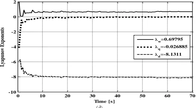
Situation 1: Assume that there are no uncertainties in the drive system, all the parameters are known. Both conventional controller and designed controller are examined. Results are shown in Figs. (3) and (4). To show the ability of designed controller, the controller in 6th _{second is put into effect. In Fig. (4), desired}

Lyapunov exponent is considered as : * *

11, 10

d q

that the proposed controller is able to stabilize the chaotic angle speed, q-axis and d-axis currents at the desired goal.

(a)

(b)

(c)

0 5 10 15 20 25 30

-40 -30 -20 -10 0 10 20 30

Time [s]



0 5 10 15 20 25 30

-80 -60 -40 -20 0 20 40 60 80

Time [s]

i q

0 5 10 15 20 25 30

-40 -20 0 20 40 60 80

Time [s]

(d)

Fig. 3. Performance of conventional controller: (a) Rotor speed; (b) q-axis current; (c) d-axis current; and (d) dynamics of Lyapunov exponents.

(a)

(b)

0 10 20 30 40 50 60 70

-10 -8 -6 -4 -2 0 2

Time [s]

L

yap

un

ov

E

xp

on

en

ts



w=0.69795

_q=-0.026885 

d=-8.1311

0 5 10 15 20 25 30

-20 -10 0 10 20 30 40 50

Time [s]



0 5 10 15 20 25 30

-100 -50 0 50 100 150 200 250

Time [s]

[image:10.595.131.460.85.267.2]

(c)

(d)

Fig.4. Performance of designed controller: (a) Rotor speed; (b) q-axis current; (c) d-axis current; and (d) dynamics of Lyapunov exponents.

Situation 2: Assume that we know the PMSM is running in chaos, but the system parameter TLis unknown, and assume that there are a sudden step change of this parameter from 1 to 5 at t=8. So we use the designed controller proposed in case (2) to control the chaotic PMSM from the starting the motor. Parameters of controller in this situation are: 15, P 10,20.33,Pq5.

(a)

0 5 10 15 20 25 30

0 5 10 15 20 25 30 35

Time [s]

i d

0 10 20 30 40 50 60 70 80 90 100

-13 -12 -11 -10 -9 -8 -7 -6 -5 -4 -3

Dynamics of Lyapunov exponents

Time [s]

L

y

a

p

u

n

o

v

e

x

p

o

n

e

n

ts _

=-5.46

_q=-10

_d=-11

0 5 8 10 15

0 2 4 6 8 10 12 14

8

Time [s]

e

s

ti

m

a

te

d

(b)

(c)

(d)

Fig. 5. Step change in TL: (a) estimated TL; (b) Rotor speed; (c) q-axis current (d) d-axis current.

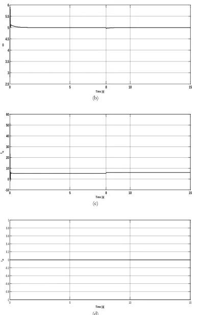
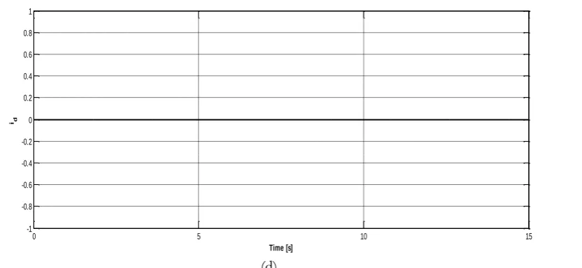
Situation 3: Assume that we know the PMSM is running in chaos, but the system parameter γis unknown, and assume that there are a sudden step change of this parameter from 20 to 30 at t=8.So we use the

0 5 8 10 15

2.5 3 3.5 4 4.5 5 5.5 6

Time [s]



0 5 8 10 15

-10 0 10 20 30 40 50 60

Time [s]

iq

0 5 10 15

-1 -0.8 -0.6 -0.4 -0.2 0 0.2 0.4 0.6 0.8 1

Time [s]

[image:12.595.110.507.84.700.2]

designed controller proposed in case(2)to control the chaotic PMSM from the starting the motor. Parameters of controller in this situation are: 15 , P10 ,20.33 , Pq 5 .

(a)

(b)

(c)

0 5 8 10 15

-5 0 5 10 15 20 25 30

Time [s]

ga

m

a

0 5 8 10 15

-1 0 1 2 3 4 5 6

Time [s]



0 5 8 10 15

-10 0 10 20 30 40 50 60

Time [s]

(d)

Fig. 6. Step change in γ: (a) estimated γ; (b) Rotor speed; (c) q-axis current; and (d) d-axis current.

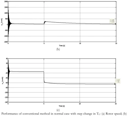
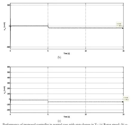
Normal mode: Now the performance of the controller in normal mode is compared with a conventional controller. Assume that the system parameter TLis unknown and there are a sudden step change of this parameter from 1 to 5 (N.m) at t=5 sec. Here dimensionless model of PMSM is not used because we don’t want to investigate chaotic PMSM, so mathematical model of PMSM in (1) is used and desired speed will be: *

100 ( )

sec rad

  . It’s clear that designed controller have better performance with less control signal effort. Figures 7 and 8 show the performance of conventional controller and designed controller, respectively. The motor parameters in normal mode (not chaotic mode) and PI gains used in the conventional controller are shown in Appendix.

(a)

0 5 10 15

-1 -0.8 -0.6 -0.4 -0.2 0 0.2 0.4 0.6 0.8 1

Time [s]

id

0 5 10 15

-20 0 20 40 60 80 100 120 140 160 180

Time [s]



[

r

a

d

/s

[image:14.595.105.522.86.278.2]

(b)

(c)

Fig. 7. Performance of conventional method in normal case with step change in TL: (a) Rotor speed; (b)

q-axis stator voltage; and (c) d-axis stator voltage.

(a)

0 5 10 15

-1500 -1000 -500 0 500 1000 1500 2000

X: 14.89 Y: 52.44

Time [s]

uq

[v

o

lt]

0 5 10 15

-140 -120 -100 -80 -60 -40 -20 0 20 40

X: 14.87 Y: -65.1

Time [s]

ud

[v

o

lt]

0 5 10 15

-20 0 20 40 60 80 100 120 140 160

Time [s]



(

r

a

d

/s

[image:15.595.103.535.87.477.2]

(b)

(c)

Fig. 8. Performance of proposed controller in normal case with step change in TL: (a) Rotor speed; (b)

q-axis stator voltage; (c) d-q-axis stator voltage.

Practical experiments can be a topic for more researches in future, and also this method can be examined on other motors which have chaotic behavior for a range of their parameters like brushless DC motors or induction motors and etc. It may be possible to combine chaos control and vector control with using other methods of controlling the chaos.

6.

Conclusion

A nonlinear vector control method is designed for the chaotic permanent magnet synchronous motors. The controller is based on the setting the desired Lyapunov exponents approach and is used to prevent the motor drive system from chaos and make it track the desired speed command. The uncertainties of the system are also considered in the design. And the stability analysis for closed loop system is derived to prove the system reliability using direct Lyapunov method. Proposed controller has been examined in both

chaotic and normal mode. In chaotic mode, simulation results prove that controller can eliminate the chaos; and also in unknown parameters case, was shown that designed controller can estimate the parametric uncertainties. In normal mode controller can control the system by using the smaller control signal effort. The system has the distinct advantages of smallercontrol signal effort and quick response.

0 5 10 15

-500 0 500

X: 14.92 Y: -49.91

Time [s] uq

[v

o

lt]

0 5 10 15

-200 -100 0 100 200 300 400 500 600

X: 14.89 Y: -48.11

Time [s] ud

[v

o

[image:16.595.99.538.84.503.2]

Appendix

The motor parameters in normal mode (not chaotic mode) and PI gains used in the conventional controller are shown in Table I [24].

Table I. System parameters.

Base voltage 179.629 V

Base current 10 A

Base electric frequency 200 Hz

Base Speed 6000 rpm

Pole pair number (

n

p) 2

Stator inductance (L) 0.0029H viscous damping coefficient(β) 0.001(N/rad/s) polar moment of inertia (j) 0.003 (kg.m2₎

Stator resistance(R) 2.2Ω Magnetic flux constant (Ψ) 1 volts/rad/sec d-axis current loop Kp = 0.5, Ki = 0.1 q-axis current loop Kp = 0.5, Ki = 0.05 Speed loop Kp =40, Ki = 0.2

References

[1] G. R. Slemon, Electric Machines and Drives. Addison-Wesley publishing, Co., Inc., 1992.

[2] T. Sun, C. Liu, N. Lu, D. Gao, and S. Xu, “Design of PMSM vector control system based on TMS320F2812 DSP,” in Proceedings of 2012 IEEE 7th International Power Electronics and Motion Control Conference-ECCE Asia, June 2-5, Harbin, China, pp. 2602-2606.

[3] F. Blaschke,“The principle of field orientation as applied to the new transvector closed-Loop control system for rotating-field machines,” Simens Review, 1972.

[4] M. A. Rahman, “On-line adaptive artificial neural network based vector control of permanent magnet synchronous motor,” IEEE Transactions on Energy Conversion, vol. 13, no. 4, Dec. 1998.

[5] M. A. El-Sharkawi, A. A. El-Samahy, and M. L. El-Sayed, “High performance drive of dc brushless motors using neural network,” IEEE Trans. on Energy Conversion, vol. 9, no. 2, pp.317-322, 1994. [6] N. Hemati, “Strange attractors in brushless DC motors,” IEEE Trans. Circuits Systems-I, vol. 41, no. 1,

pp. 40-45, Jan. 1994.

[7] Z. Li, J. B. Park, Y. H. Joo, B. Zhang, and G. Chen, “Bifurcations and chaos in a permanent-magnet synchronous motor,” IEEE Trans. Circuits Systems-I, vol. 49, no. 3, pp. 383-387, 2002.

[8] A. Rasoolzadeh and M. Tavazoei, “Prediction of chaos in non-salient permanent magnet synchronous machines,” Physics Letters A, vol. 377, no. 1-2, pp. 73-79, Dec. 2012.

[9] Z. Jing, C. Yu, and G. R. Chen, “Complex dynamics in a permanent-magnet synchronous motor model,” Chaos, Solitons and Fractals, vol. 22, no. 4, pp. 831-848, Nov. 2004.

[10] O. Calvo and J. H. E. Cartwright, “Fuzzy control of chaos,” International Journal of Bifurcation & Chaos, vol. 8, no. 8, pp. 1743-1747, 1998.

[11] S. Takanori, I. Sanae-I, and Y. Masatoshi, “Control of chaos by linear and nonlinear feedback method,” J. Plasma Fusion Res. Series, vol. 6, pp. 263-266, 2004.

[12] H. T. Yau and C. K. Chen, “Sliding mode control of chaotic systems with uncertainties,” International Jornal of Bifurcation & Chaos, vol.10, no. 5, pp. 1139-1147, 2000.

[13] E. Ott, C. Grebogi, and J. A. Yorke, “Controlling chaos,” Phys. Rev Lett, vol. 64, pp. 1196-1199, 1990. [14] B. Zhang, Z. Li, and Z. Y. Mao, “Anti-control of its chaos and chaos characteristics in the

permanent-magnet synchronous motors,” Control Theor. Appl., vol. 19, 2002. (in Chinese)

[15] H. Ren and D. Liu, “Delay feedback control of chaos in permanent magnet synchronous motor,” in

[16] H. Ren and D. Liu, “Nonlinear feedback control of chaos in permanent magnet synchronous motor,”

IEEE Trans Circuits and syst-II, vol.53, no.1, pp. 45-50, 2006.

[17] W. Kinsner, “Characterizing chaos through Lyapunov metrics,” IEEE Trans Syst Man Cybernetics-Part C, vol. 36, no. 2, pp. 141–51, 2003.

[18] A. Wolf, J. B. Swift, H. L. Swinney, and J. A. Vastano, “Determining Lyapunov exponents from a time series,” Physica D, vol. 16, pp. 285–317, 1985.

[19] M. Zribi and A. Oteafy, “Controlling chaos in the permanent magnet synchronous motor,” Chaos, Solitons and Fractals, vol. 41, pp. 1266–1276, 2009.

[20] V. Kordic, Kalman Filter. InTech, May 2010.

[21] S. Vaez-Zadeh and E.Jalali “Combined vector control and direct torque control method for high performance induction motor drives,” Energy Conversion and Management, vol. 48, pp. 3095-3101, 2007. [22] M. Ataei, A. Kiyoumarsi, and B. Ghorbani, “Control of chaos in permanent magnet synchronous

motor by using Lyapunov exponents placement,” Physics Letters A, vol. 374, no. 41, pp. 4226-4230, 2010.

[23] F. A. C. C. Fontes and L. Magni, “A generalization of Barbalat’s lemma with applications to robust model predictive control,” in Proceedings of 16th _{International Sympsium on Mathematical Theory of Networks} and Systems, Katholieke Universiteit Leuven, Belgium, Jul. 2004.