Robust real-time substructuring techniques for under-damped systems

White Rose Research Online URL for this paper:

http://eprints.whiterose.ac.uk/79699/

Version: Submitted Version

Article:

Gawthrop, P.J., Neild, S.A., Wallace, M.I. et al. (1 more author) (2007) Robust real-time

substructuring techniques for under-damped systems. Structural Control and Health

Monitoring, 14. 591 - 608. ISSN 1545-2255

https://doi.org/10.1002/stc.174

Reuse

Unless indicated otherwise, fulltext items are protected by copyright with all rights reserved. The copyright exception in section 29 of the Copyright, Designs and Patents Act 1988 allows the making of a single copy solely for the purpose of non-commercial research or private study within the limits of fair dealing. The publisher or other rights-holder may allow further reproduction and re-use of this version - refer to the White Rose Research Online record for this item. Where records identify the publisher as the copyright holder, users can verify any specific terms of use on the publisher’s website.

Takedown

If you consider content in White Rose Research Online to be in breach of UK law, please notify us by

for under-damped systems

P. J. Gawthrop

_{, M. I. Wallace}

_{, S. A. Neild}

_{, and D. J. Wagg}

1_{Centre for Systems and Control and Department of Mechanical Engineering, University of Glasgow, GLASGOW. G12 8QQ}

UK

2

Department of Mechanical Engineering, Queens Building, University of Bristol, Bristol BS8 1TR, UK.

SUMMARY

This paper considers the hybrid simulation of under-damped dynamical systems using numerical-experimental real-time substructuring. Substructuring joins together a physical plant with a numerical model using real time control techniques, such that the combined model emulates the behaviour of the entire system. Due to the low damping, the control of substructured systems can be highly sensitive to delay and uncertainty. We present a technique for calculating the critical delay of the substructured system using a phase margin approach. In addition, it is shown that robustness techniques, drawn from feedback control theory, can be used to reduce the destabilizing effect of uncertainty. To demonstrate this a comparison of three different robustness compensators is presented, using a well known linear system. The level of uncertainty is deliberately increased to compare their performances and a discussion is made on when each may be most useful. Copyright c°2005 John Wiley & Sons, Ltd.

KEY WORDS_{: Hybrid testing, substructuring, stability, robust control}

∗_{Correspondence to: P. .J .Gawthrop, Centre for Systems and Control and Department of Mechanical Engineering, University of}

1. Introduction

In this paper we consider the recently developed structural testing method of real-time dynamic

substructuring. This is a form of hybrid numerical-experimental testing suited to testing large structures

or complex systems containing acritical componentof interest [13]. The technique allows the critical

component to be tested experimentally at full scale while the remainder of the system is modelled

numerically. The coupling between the physical and numerical parts is achieved using real-time control

of actuators connected to the physical substructure [1, 2, 6, 9].

As pointed out previously [4, 10], substructuring can be viewed as a control problem. However,

unlike conventional control system design which aims for a well-damped closed-loop system, the

corresponding substructuring design often has lightly-damped behaviour near the boundary of stability.

For this reason,robustnessis an essential consideration for this type of testing. However, because the

testing technique has been developed primarily from a civil engineering perspective, robustness has

not been studied using a control theoretic approach. In this paper we apply tools from control theory

to study the robust stability of a generic linear substructuring system. In particular we focus on the

effect of unmodelled delays and other uncertainties which occur during substructuring. We present

a technique for calculating the critical delay,τc, beyond which the substructured system will become

unstable, characterized by the onset of oscillations with positive exponential growth. Another approach

for identifying this critical delay is presented by Wallace et al. [11] which uses Delay Differential

Equation (DDE) models to analyse the substructured system; the relation between the two approaches

is discussed in this paper.

12]. These strategies consist of compensating for the combined dynamics of the actuator(s) and

corresponding proprietary (i.e. built in) controller(s) — together these are referred to as thetransfer

system(s). An additional compensator (or outer-loop controller) is introduced around the transfer

system to eliminate the effect of its own dynamics from the force fed back from the substructure.

The outer-loop controllers suggested to date broadly fall into two categories, those that provide (time)

delay (e−sT) compensation and those that provide lag (e.g.₁₊1_sT) compensation; section 2 presents more

detail on these outer-loop strategies.

In this paper, the problem of robustness is considered for a generic substructuring model. In

particular, robustness is a particular concern when the structure being tested is lightly damped or

there is a high level of uncertainty in the transfer system control. Here we examine the stability and

robustness of a substructuring algorithm and describe a strategy for increasing the control robustness

for lightly-damped systems through the use of a robust transfer system design methodology. Three

types of robustness compensators are proposed to address uncertainties in the transfer system model.

The trade off is that control performance (in terms of accuracy of the hybrid simulation) is reduced

for increased control robustness. The effects of the robustness compensators are illustrated using a

single degree-of-freedom example, with both hybrid numerical-experimental results compared to pure

numerical simulations, by intentionally increasing the uncertainty in the system.

2. The substructuring algorithm

To carry out a substructuring test, the numerical model and the physical substructure are run in parallel

and interact in real-time to emulate the dynamic behaviour of the complete structure. This interaction

is achieved through the exchange of information at the interface between the numerical model and

using a numerical model and imposed via actuation devices (the transfer systems) on the physical

substructure. Secondly, the forces due to imposing these displacements on the physical substructures

are measured and fed back to the numerical model where they are included at the interface for the

next time step. A controller is used to minimize the effects of the dynamics introduced by the transfer

system. Most dynamic test methods use a proprietary controller, which typically performs PID control,

to reduce the uncertainty of the transfer system dynamics to an acceptable level. However, to achieve

a stable substructuring algorithm a more sophisticated compensation scheme is also required to reduce

the delay introduced by the transfer system to a level below the critical limit.

The first time delay compensators were obtained by assuming that the dynamics of the transfer

system may be approximated to a pure delay. For example, Horiuchi et al. [6] and Blakeborough et al.

[1] proposed outer-loop forward prediction methods which use polynomial extrapolation to predict

forward the numerical model displacement by a fixed number of time-steps. Darby et al. [2] relaxed the

assumption of a pure delay by developing a forward prediction method that varied the amount of delay

compensation, based on the error between the actuator displacement and the desired numerical model

displacement. This method was extended by Wallace et al. [12] who developed an adaptive forward

prediction algorithm that used variable polynomial coefficients such that non-integer multiples of the

previous time step could be predicted and also incorporates an amplitude correction algorithm. The use

of a Smith predictor has also been proposed as a suitable delay compensator [9].

Lag compensation via an experimental transfer function estimation of the combined inner-loop

controller and actuator dynamics has been proposed by Gawthrop et al. [4] and Reinhorn et al. [9].

The proposed outer-loop controllers compensate for unwanted dynamics by applying the inverse of

the transfer function estimation. Model reference adaptive control has also been suggested as an

compensation can be achieved via this approach.

Noting that bothe−sT and₁₊1_sT have the same first-order Taylor expansion (1−sT) – which indeed

they share with more complicated transfer functions such as 1

(1+sT 2)2

and (1−s T 2) 1+sT

2

– there is not much

practical difference between the approaches when the damping is small as low order approximations

apply in this case. This point is examined further in Section 3.1.

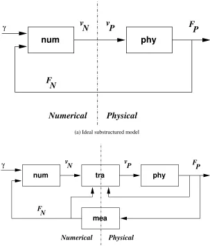
[Figure 1 about here.]

Figure 1 shows two block diagram representations of substructuring†. Figure 1(a) shows the ideal case

where a numerical substructure,num, is coupled directly to a physical substructure,phy, and there

are no transfer system dynamics and hence no need for a controller. The detail of the two substructure

blocks is: forphythe outputFpand inputdPare a collocated force and displacement pair connecting

phyto the numerical part of the substructured system. Similarly fornumthe outputFN and inputdN

are the collocated force and displacement pair connectingnumto the physical part of the substructured

system. The signalrrepresents the net effect of external forces in the numerical part of the model.

In this ideal situation,FN=FPanddP=dNand the dynamic behaviour of the substructured system

exactly replicated that of the emulated system‡. However, for structural or mechanical systems, the

physical system input dP has to be generated by a transfer system which has the control objective

of settingdP≈dN. The physical force FP is measured by asensor system which also has it’s own

dynamics. In practice the ideal sensor system has the relationship thatFP→FN asdp→dN.

Figure 1(b) gives a block diagram representation of the practical case. In addition to the two blocks

of Figure 1(a);trarepresents the controlled transfer system including both inner- and outer-loop control

†_{An alternative bond graph representation is given by Gawthrop et al. [4].}

‡

This is the case in Hardware-in-the-loop testing, where because of the structure of the system being tested, the transfer systems

systems, andmearepresents the measurement sensor system, which includes the force transducer and

associated power supplies (this is assumed not to interact withphy). We note that physical part oftra

usually consists of the actuator and inner-loop controller and is affected byFP(an actuator only has a

finite performance capacity envelope in which it will operate in a linear fashion), while the numerical

(augmented) part oftrais the outer-loop controller and robustness compensator with its accuracy being

affected by the measured version ofFP(FN). At this point, the following assumption is made

Assumption 1. The four systems in Figure 1(b) arelinear,time-invariantandstable.

Using Assumption 1, the ideal substructuring case, Figure 1(a), may be represented by:

FP=P(s)dP (phy), (1)

dN =N1(s)r−N2(s)FN (2)

=N(s)(Nr(s)r−FN) (num), (3)

where,P(s)is the transfer function corresponding tophy,N1(s)andN2(s)in Equation (2) are separate

parts of the numerical model, which we re-express in Equation (3) in a more convenient form for

later analysis;N(s)is the transfer function corresponding to num andNr(s)is a transfer function

representing the interface betweennumand the external forcing. In the ideal case there are no transfer

system or measurement dynamics, such that FN =FPanddP=dN. Then Equations (1) and (3) for

the physical substructure and the numerical model dynamics may be simplified such that the overall

system dynamics are identical to that of the emulated system. This leads to the relation

FP=

L0(s)

1+L0(s)Nr(s)r, (4)

whereL0(s) =P(s)N(s)and is defined as thenominalloop gain.

the measurement system must be included. We define these dynamics as

dP=T(s)dN−TP(s)FP (tra), (5)

FN=M(s)FP (mea), (6)

where the termTP(s)FPof Equation (5) includes theneteffect ofFPandFNontra. From Assumption 1,

each transfer function explicitly appearing in Equations (1)–(6) isstable. The issue is then to investigate

whether the dynamics of the substructured system shown in Figure 1(b) is also stable.

Rearranging equations (1), (3), (5) and (6) the representation of Figure 1(b) may be written as

[1+P(s)Tp(s)]Fp=L0(s)[T(s)Nr(s)r−T(s)M(s)Fp]. (7)

Defining theneglectedgain asΛ(s)and theneglectedforward gain asΛr(s)we obtain

Λ(s) = [1+P(s)TP(s)]−1T(s)M(s), (8)

Λr(s) = [1+P(s)TP(s)]− 1

T(s)). (9)

Defining anequivalentforce,Fe=Λr(s)Nr(s)r, the system dynamics may be expressed as

FP=L0(s)[Fe−Λ(s)FP]. (10) Figure 1(b) can thus be represented by the classical feedback system of Figure 2.

[Figure 2 about here.]

Finally, definingD(s)as the transfer function relatingFeandFPfor the practical substructured system,

using (10) we can write:

D(s) = L0(s)

1+Λ(s)L0(s), (11)

such that

Using Equation (4) and recognising that for the ideal caseΛ(s) =Λr(s) =1, the corresponding nominal transfer function relating to the ideal substructured system, and the emulated system, may be defined

as

D0(s) = L0(s)

1+L0(s). (13)

In Section 4 we discuss the use of different robustness compensation schemes. We note that D0(s)

will explicitly include these algorithms and therefore change. Thus for comparison, we defineDemas

the emulated system transfer function such that Dem=D0(s)when L0(s) does not incorporate any

compensation schemes.

3. Relative and robust stability

Figure 2 and the corresponding closed-loop system (12) are in the classical feedback control system

form where L0(s) would be interpreted as the “system” and Λ(s) as the “controller”. This means

that a range of standard control system design techniques (Goodwin et al. [5] gives a comprehensive

exposition) can be brought to bear on the problem.

For example,relative stability [5, sec. 5.8] can be characterized as follows. Define the critical

frequencyωcas the solution of

|L(jωc)|=1, (14)

where theactualloop gain,L(s), is defined as

L(s) =Λ(s)L0(s). (15)

The correspondingphase marginφmmay be written as

The phase margin provides a measure of how near to instability the ideal system (whereΛ(s) =1) is in

terms of how much phase lag (due toΛ(s)6=1) is permissible. For example, if the neglected dynamics

comprise a pure delay (Λ(s) =e−sτ_{) then thecritical delay,τ}

c, is the time delay which would give a

phase lag ofφmand is given by

τc=

φm

ωc

. (17)

This gives an alternative method for computing the critical delay, in addition to that developed by

Wallace et al. [11] which uses Delay Differential Equation (DDE) models. For the class of system for

which the DDE methods cannot be applied or when it is impractical to use the technique, Equation

(17) could still be used in many cases (even if only as a linear approximation) to give an estimate ofτc. The link between the two techniques is discussed further in Section 3.1.

For substructuring systems in the form developed in Section 2 we would like to apply more general,

robust stabilitymethods. Using the approach outlined in [5, sec. 5.9], together with the assumption that

bothL0(s)andΛ(s)are stable implies that the closed-loop system of Figure 2 is stable if

|D0(jω)||∆(jω)| ≤1 ∀ω, (18)

where

∆(s) =Λ(s)−1. (19)

This is a conservative result but has the advantage of bounding the error transfer function∆in terms of

the desired systemD0(jω). In particular is shows that∆(jω)must be small at those frequencies where

D0(jω)is large — typically at the resonant frequencies of the desired system.

Although these methods are standard in the control system context, they are novel in the

substructuring context. In particular, both relative and robust stability can be reinterpreted for

3.1. Substructuring Example

[Figure 3 about here.]

[Figure 4 about here.]

[Figure 5 about here.]

An example of a substructured system is shown schematically in Figure 3. The system has

a numerical substructure consisting of a mass of mkg, a spring with stiffness kN/m and damper

with constant cNs/m and a physical substructure consisting of a spring with stiffness ksN/m. This

corresponds to the hybrid numerical-experimental system which will be presented in Section 5. In this

case

L0(s) = ks

ms2_+cs+k, (20)

Nr(s) =cs+k. (21)

Defining the natural frequency of the numerical subsystem asωn=

q

k

m, the corresponding damping

ratioζ= c

2mωn andp= ks

k we can write

L0(s) = pω 2 n

s2_+2ζω ns+ω2n

, (22)

Nr(s) =m(2ζωns+ω2n). (23) Defining ˆs=_ωs_n, this can be rewritten in normalised form as

L0(s) = p ˆ

s2_+2ζsˆ+1, (24)

Nr(s) =k(2ζsˆ+1). (25) Defining ˆω=_ωω

n and using (14), the critical frequency corresponding to (24) is the solution of

Equation (26) is quadratic in ˆω2

. It has real solutions if

(4ζ2−2)2>(1−p2). (27)

There are two cases: ifp_≥1 then Equation (27) is independent ofζ, otherwise the condition depends

on the value ofζ. In the case of real solutions, the positive square root of a positive solution gives a

(positive) value of ˆωsatisfying Equation (14).

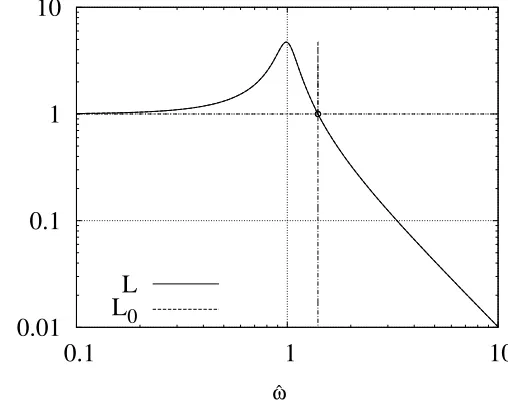
Figure 4(a) shows log|L0(jωˆ)|plotted against jωˆ forp=1 andζ=0.107. In this case, ˆωc=1.398, the frequency at which|L0(jωˆ)|=1. Figure 4(b) gives the corresponding phase (in degrees) indicating a phase margin of 17.34◦=0.3027rad. This gives a critical delay of ˆτc=0.2165, which is precisely the value obtained from the DDE numerical analysis of Wallace et al. [11] confirming the fact that both

methods are exact. However, the method of this paper gives a different insight into the problem and

has a number of advantages: it can be used for more complicated examples than can the DDE approach

and is applicable to uncertainties modelled byanytransfer function.

The corresponding diagrams forL=e−jωˆ_L

oare plotted in Figures 4(a) and 4(b). As predicted,

L(jωˆc) =−1 corresponding to|L(jωˆc)|=1 and∠L(jωˆc) =−180◦.

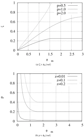
Figure 5(a) shows how the phase margin varies withζand 5(b) how it varies withp. For small values

ofζ, the phase marginφmis approximately proportional toζ. Larger values ofpgive a reduced phase

margin. Figure 4(a) also provides alternative insight into the solution of Equation (26). From Equation

(24), the sole effect of pis to move the curve of Figure 4(a) vertically. It is therefore clear that when

p>1, log|L0(jωˆ)|=0 at only one frequency implying a single positive real solution of Equation (26) for ˆω2

. On the other hand, ifp<1 there is no solution if the peak of the curve is below zero. From

Equation (24), the peak value occurs at an approximate frequency of ˆω=1 where|L0(jωˆ)|=₂p_ζ. Thus, as also indicated in Figure 5(b), the phase margin is infinite whenp<2ζ.

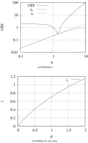
The robustness criterion Equation (18) can be examined by plotting both _|D(1_jωˆ)| and|∆(jω)| on

the same diagram. For example, Figure 6(a) shows _|D(1_jωˆ)| when p=1 andζ=0.107. On the same

diagram,|∆(jω)|is plotted for two cases:

Λ(sˆ) =



   

   

e−τˆsˆ, (shown as∆din Figure 6(a)) 1

1+ˆτsˆ, (shown as∆lin Figure 6(a))

(28)

where ˆτ=0.21. In this case, stability is predicted in each case as Equation (18) is satisfied. However,

this would not be the case ifτwere increased slightly. Note that both forms ofΛ(sˆ)of Equation (28)

give similar results in this case indicating thatphaseerror is more important thatamplitudeerror in

this case. Note that ˆτ=0.21 predicted by this (conservative) robust stability method is less than that predicted by the the exact relative stability (phase margin) approach. However, the robustness approach

is more general in that the uncertainty does not need to be parameterized by a transfer function.

The minimum value of_|D(1_jωˆ)|occurs at ˆω2

≈(1+p)with a value of approximately 2ζ√_p1+p. Noting

that the maximum value of∆=1−e−ˆτsˆis 2, it follows that the substructured system will be stable for

anydelayτif

ζ>√ p

1+p. (29)

Figure 6(b) shows the boundary implied by Equation (29).

4. A Robust Transfer System Design Methodology

This paper provides a stability and robustness analysisof the substructuring problem by applying

techniques from linear control theory. This leads on to a methodology for thedesignof the transfer

system to achieve robust stability. The use of linear theory — and particularly the assumptions that the

at first sight appear to be a serious limitation of this analysis. However, these results can be applied to

— and in some cases can significantly improve results from — substructuring tests with nonlinear

elements. This is because a robust linear system can cope with a significant amount of nonlinear

‘disturbance’. Using this approach we are able to get a good comparison of results between three

different types of robustness compensator — shown in section 5.

Using linear analysis, we propose a 4 stage controller design strategy for each transfer system (which

in this work we assume to be an actuator):

1. Design an (or use the proprietary) inner-loop controller around the actuator to reduce

uncertainty and non-linearity in the resultant closed-loop transfer system.

2. Use system identification to estimate a (closed-loop) transfer function of the actuator and

inner-loop controller (which we define as thenominalmodel). Use the same system identification

results to estimate anuncertaintymodel for the transfer system.

3. Use the nominal model from step 2 to design an outer-loop transfer system cancellation

controller.

4. Use theuncertaintymodel from step 2 to design a robustness compensator.

Broadly, the literature outlined in Section 2 addresses steps 1–3; the selection of the inner-loop

controller gains, a system identification of the resulting transfer system and the design of an

outer-loop controller to compensate for the transfer system dynamics. The adaptive nature of the outer-outer-loop

controllers proposed in [2, 8, 12] allow for the compensation of the transfer system dynamics despite

uncertainty in the transfer function model derived in step 2. Although they incorporate some level of

robustness due to this adaptation, they do not explicitly include the robustness compensator proposed

in step 4. This is the key reason why the linear results can be applied so readily to systems where the

adaptive forward prediction of Wallace et al. [12]) plus the robustness compensation allows the system

to cope with a significant degree of nonlinear ‘disturbance’. We note also that the analysis applies

primarily to the design of the transfer system. In fact we wish to design a stable robust control strategy

to eliminate (or at least mitigate) the effect of uncertainty and non-linearity from the transfer system —

we want to make the transfer system dynamics linear. The only time we actually require a definition of

the transfer function of the physical substructure (which is usually a nonlinear element [13]) is in order

to apply the robustness compensation technique based on physical model emulation, as described in

Section 4.3.

From Section 3, it is clear that instability can still occur even in the presence of apparently quite

small neglected dynamics; in other words, the nominal design is not necessarily robust. However, the

trade off for achieving a robust system is a reduced level ofnominalperformance.

There are three approaches suggested here

1. Damping-ratio compensation:ζ-robustness

2. Phase-advance compensation:α-robustness

3. Physical model emulation:γ-robustness

All three approaches have a single parameter which provides a trade-off between performance and

robustness and are considered in the following sections. Section 4.4 gives a specific example. Methods

1 and 3 are believed to be new and have been developed specifically with substructuring in mind

[4, 12]; method 2 is a standard control system technique [5, section 6.6] applied here for the first time

to substructuring. Method 3 is related to the Youla parametrisation of all stabilising controllers [5,

4.1. Damping-ratio compensation:ζ-robustness

From Figure 6(a), it is clear that it is the magnitude of the resonant peak of the closed-loop transfer

function|D0(jωc)| that restricts the maximum allowed value of uncertainty|Λ(jωc)|. As|D0(jωc)| decreases with increasing damping, a simple way of trading robustness for stability is to increase the

damping coefficients of the numerical model above their correct values.

This method has the advantage of requiring no knowledge about the system properties but has the

disadvantage of distorting the nominal closed loop system.

4.2. Phase-advance compensation:α-robustness

The example of Section 3.1 implies that lack of robustness is due to the neglected phase lag associated

withΛ(jω)atw=ωc. One way to improve robustness is to deliberately introduce phase advance, at

the critical frequency, toΛ(jω)by interposing a phase advance transfer function between numand

tra. Perhaps the simplest such transfer function is [5, sec. 6.6]:

C(s) =α₁s+ωc

αs+ωc

(30)

where the parameterα≥1. Clearlyα=1 corresponds to a unit transfer function which has no effect;

the maximum phase advance occurs at aboutω=ωc. The maximum phase advance rises to about

π

4rad=45owhich whenα≈10 [5, sec. 6.6]. Typically, for this application, 1<α<2.

This method has the advantage of requiring only knowledge of ωc, but has the disadvantage of

distorting the nominal closed loop system.

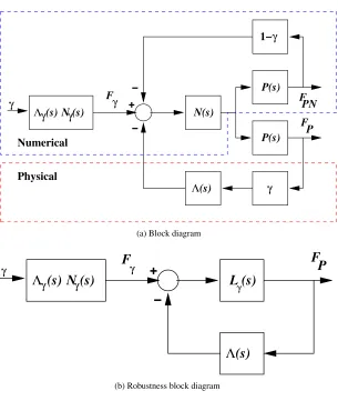
4.3. Physical model emulation:γ-robustness

[Figure 7 about here.]

subsystem. As indicated in block diagram form in Figure 7(a), the output ofnumis fed into both the

simulation ofphyand the physical subsystemphy. In comparison to Figure 2, there aretwofeedback

loops:γtimes the output of the physical system and(1−γ)is fed back to the input of the numerical

subsystem. At the two extremes,γ=0 gives a purely numerical simulation (andΛ(s)is not part of the

feedback), whereasγ=1 gives the hybrid numerical/physical simulation discussed in the preceding

sections. When 0_≤γ_≤1, there is a smooth transition between the two extremes. However, for each

value ofγ, thenominalclosed loop system dynamics are the same.

The block diagram of Figure 7(a) can be rewritten in the simplified form of Figure 7(b) where

Lγ(s) = γ

L0(s)

1+ (1−γ)L0(s). (31)

The robustness results of Section 2 can then be applied to Figure 7(b) in a similar way as to that

discussed for Figure 2.

This method has the disadvantage of requiring an accurate model of the physical system transfer

functionP(s)but has the advantage ofnotdistorting the nominal closed loop system.

4.4. Example (continued)

[Figure 8 about here.]

Figure 8(a) is the same as Figure 6(a) except that the results of each of the three compensators are

shown as well. In each case, the stability margin is significantly increased at the resonant frequency; in

each case, ˆτ≈0.35, about0.35

0.21=1.67 larger than the uncompensated case.

Figure 8(b) shows the closed loop system when the actual system (comprising the nominal system

and the time delay) is compensated by the three robustness compensators. Although, as expected, these

three closed-loop responses differ from the nominal (D0) they are better than the uncompensated case

The other observation from Figure 8(a) is that there are significant differences between 1/|D_|for the

three different compensation methods. This will be discussed in more detail in relation to the hybrid

numerical-experimental results shown in the next section.

5. Hybrid testing

[Figure 9 about here.]

The proposed robustness methods were evaluated using a small-scale substructuring experiment

of the system described in Section 3.1. For the experiments, the numerical model and outer-loop

compensator were written in the Matlab Simulink environment and run in real-time on a DSP using a

dSpace DS1104 Controller Board. The transfer system is a linear electro-mechanical actuator attached

to a centralising plate which is free to run via linear bearings on three guide rails, as shown in Figure

9. The physical substructure is a spring of stiffnessks=2250Nm−1, which is held rigid at one end and

attached to the actuator centralising plate via a load cell at the other.

5.1. Robust Transfer System Design

The experimental equipment has been extensively analysed and it is known that a good model for the

neglected dynamics of the system under an inner-loop proportional (P) control withkp=1 is a pure

delayΛ(sˆ)≈e−sˆˆτwhere ˆτ≈0.29. Using the parameters for this example and Equation (17) the critical

value of the delay is found to be ˆτc≈0.2. Therefore this system isunstablewithout some form of

delay compensation because ˆτ>τˆc. In this present study we are interested in robustness, therefore we will use the delay compensation method of Wallace et al. [12] as step 3 of the robust transfer system

within the stable range of 0≤ˆτ<ˆτc by varying the parameters of the delay compensation scheme. This is a simple way of varying the degree of uncertainty in the system, and gives an indication of the

performance of each robustness compensator as uncertainty increases.

[Table 1 about here.]

Table I summaries the values of ˆτused to generate the hybrid numerical-experimental results shown

in Figures 10–12. For each ˆτvalue, Table I shows the ratio ˆτ/τˆcto give an indication of how close the system is to the stability boundary at ˆτ/τˆc=1.

5.2. Numerical-experimental results

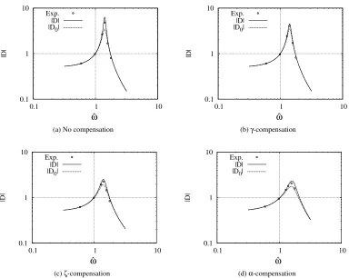
Each of Figures 10–12 shows hybrid numerical-experimental results for four cases: no compensation,

γ-compensation, ζ-compensation and α-compensation. Each plot shows three sets of data. Circles

correspond to hybrid numerical-experimental measurements of|D(jωˆ)|(11) at six frequencies: 3.0Hz,

5.0Hz, 6.5Hz, 7.1Hz, 8.0Hz and 9.0Hz. The solid and dashed lines are the theoretical values of|D(jωˆ)|

(withΛ(sˆ)≈e−sˆτ) (11) and|D0(jωˆ)|(whereΛ(sˆ) =1) (13) respectively.

[Figure 10 about here.]

Figure 10 shows the case where ˆτ=0 (i.e. the delay compensation method is removing the full 9.4ms

of delay in the system). In this case|D(jωˆ)|and|D0(jωˆ)|are indistinguishable and the uncertainty is

very low such thatΛ≈1 and|D_{| ≈ |}D0|. With no compensation (Figure 10 (a)) there is good agreement

between the hybrid numerical-experimental results and|D0(jωˆ)|, indicating (as expected) that for this hybrid test setup the delay compensation method of Wallace et al. [12] provides a significant degree

of robustness without an additional compensator. Figure 10 (b) shows theγ-compensation case where

show theζ-compensation andα-compensation respectively. In each case the robustness is improved —

indicated by an increased phase margin — but|D0(jωˆ)|is distorted. Agreement with the hybrid test

results is good although theα-compensation looses some correlation near resonance.

[Figure 11 about here.]

Figure 11 shows the case where ˆτ=0.1. This case corresponds to the situation when the delay

compensation method (step 3 in Section 4) is not fully compensating for the delay error. This can be

seen in Figures 11 (a)-(d) as the discrepancy between|D_|and|D0|close to resonance. Now without

any robustness compensation, the resonance peak|D(jωˆ)|becomes significantly exaggerated near the

resonant frequency compared to the nominal case|D0(jωˆ)|. In Figures 11 (b)-(d) the three robustness

compensators results are shown. Theγ-compensation results give a significant improvement in reducing

|D(jωˆ)|to|D0(jωˆ)|. Theζ-compensation andα-compensation also achieve the same effect, but with significant distortions in the|D0(jωˆ)| transfer function. In all three compensation cases the hybrid results match well with|D(jωˆ)|.

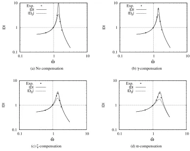
[Figure 12 about here.]

Figure 12 shows the case where ˆτ=0.19. This case corresponds to the situation when the delay

compensation method is stabilising the system, but leaving a significant delay error – corresponding to

a higher degree of uncertainty in the system. This can be seen clearly in Figure 12 (a) where now

the discrepancy between |D(jωˆ)| and |D0(jωˆ)| is even more pronounced close to resonance. The compensation methods shown in Figures 12 (b)–(d) all help to reduce this significantly. As with the

previous example the hybrid results correlate well with|D(jωˆ)|across the frequency range considered. The robustness compensation schemes can therefore be summarized by the following strengths and

γ-compensation has the advantage of not modifying the overall system response but is based on having an accurate model of the physical system – this was available for the experimental

considered here but would not generally be available. In less well known experimental

equipment, details ofΛ(sˆ)would be unknown and thus initial experiments would useγ=1.

γcould then be decreased as more experimental results allowed reduction of the uncertainty

encapsulated inΛ(sˆ).

ζ-compensation does not require a model of the physical system but does change the overall system characteristics; however, it has a clear physical meaning as a numerical model with an increased

damping ratio.

α-compensation again does not require a model but does distort the the overall system characteristics significantly.

6. Conclusion

Hybrid testing of under-damped dynamical systems using numerical-experimental real-time

substructuring is sensitive to both transfer system delay and uncertainty. The four stage robust transfer

system design methodology presented in the paper is designed to reduce both of these destabilizing

effects.

A phase margin approach to calculating the relative and robust critical delay is presented in Section

3, such that a cancellation controller (step 3) can be designed to ensure the stability of the substructuring

algorithm when there is zero uncertainty in the nominal model of the transfer system. However, due

to the characteristic nature of experimental testing, uncertainty is never negligible, especially the first

from feedback control theory can reduce this destabilizing effect. Three methods for reducing the effect

of uncertainty are discussed using theoretical and experimental results in Section 5, which show that

each is effective in increasing robustness to uncertainty.

A pragmatic view of robustness is that the amount of compensation would be large for initial

experiments, but would reduce as uncertainty was reduced. For example, using an advanced system

identification technique as suggested by Gawthrop et al. [4] or when using an adaptive cancellation

controller for step 3 of the robust transfer system design methodology. It should be noted that the lower

the damping in the system the greater the destabilizing the effect both the transfer system delay and

uncertainty have on the substructuring algorithm.

Noting that the linear robustness criterion (18) is closely related to the small-gain theorem and

circle criterion [3] for nonlinear systems, we believe that the approach can be rigorously extended to

the non-linear case.

ACKNOWLEDGEMENT

Peter Gawthrop is a Visiting Fellow at Department of Mechanical Engineering, University of Bristol.

references

[1] A. Blakeborough, M. Williams, A. Darby, and D. Williams. The development of real-time substructure testing.Philosophical Transactions of the Royal Society pt. A, 359(1869-1891), 2001.

[2] A. Darby, M. Williams, and A. Blakeborough. Stability and delay compensation for real-time substructure testing.ASCE Journal of Engineering Mechanics, 128:1276–1284, 2002.

[4] P. Gawthrop, M. Wallace, and D. Wagg. Bond-graph based substructuring of dynamical systems.Earthquake Engng Struc. Dyn., 34(6):687–703, May 2005. URLhttp://dx.doi.org/10.1002/eqe.450.

[5] G. Goodwin, S. Graebe, and M. Salgado.Control System Design. Prentice Hall, 2001.

[6] T. Horiuchi, M. Inoue, T. Konno, and Y. Namita. Real-time hybrid experimental system with actuator delay compensation and its application to a piping system with energy absorber. Earthquake Engng Struc. Dyn., 28:1121–1141, 1999.

[7] C. Lim, S. Neild, D. Stoten, C. Taylor, and D. Drury. Using adaptive control for dynamic substructuring tests. InThirteenth World Conference on Earthquake Engineering, Vancouver, August 2004. Paper No 2529.

[8] S. Neild, D. Drury, and D. Stoten. An improved substructuring control strategy based on the MCS adaptive control algorithm. Proceedings of the Institution of Mechanical Engineers Pt. I: Journal of Systems and Control Engineering, 2005. (Accepted).

[9] A. Reinhorn, M. Sivaselvan, Z. Liang, and X. Shao. Real-time dynamic hybrid testing of structural systems. InThirteenth World Conference on Earthquake Engineering, Vancouver, August 2004. Paper No 1644.

[10] D. Wagg and D. Stoten. Substructuring of dynamical systems via the adaptive minimal control approach. Earthquake Engng Struc. Dyn., 30(6):865–877, June 2001.

[11] M. Wallace, J. Sieber, S. Neild, D. Wagg, and B. Krauskopf. A delay differential equation approach to real-time dynamic substructuring.Earthquake Engng Struc. Dyn., 2005. (Accepted).

[12] M. Wallace, D. Wagg, and S. Neild. An adaptive polynomial based forward prediction algorithm for multi-actuator real-time dynamic substructuring.Transactions of the Royal Society, May 2005. (Accepted).

List of Figures

1 Substructuring: block diagram approach . . . 23

2 Sensitivity feedback system . . . 24

3 A substructured system. . . 25

4 Sensitivity: Phase margin. (a) shows the log magnitude of the nominal log|L0| and

actual log|L_|plotted against log normalised frequency log ˆω; because there is only a phase error (pure delay), the curves are the same; the critical frequency ˆωcis marked by a vertical line and a unit gain by a horizontal line. (b) shows the corresponding phases together with a vertical line at the critical frequency ˆωcand a horizontal line at−180◦.

The phase margin is the vertical distance between−180◦and the corresponding phase

curve∠L0(jωˆ)at ˆω=ωˆc. In this case, the actual system is such that the neglected time

delay is on the boundary of stability. . . 26

5 Sensitivity: dependence on parameters. (a) shows how the phase marginφm depends

onζfor three values ofp; in this case, the phase marginφmincreaseswithζ. (b) shows

how how the phase marginφmdepends onpfor three values ofζ; in this case, the phase

marginφmdecreaseswithp. . . 27

6 Robustness. (a) Shows the inverse magnitude ofD(jωˆ)against jωˆ on a logarithmic

scale. For comparison two possible uncertainty transfer functionse−jωˆτˆand₁₊1_jωˆˆτare

plotted for ˆτ=0.21. (b) Shows the boundary of stability foranydelay. . . 28

7 γ-robustness . . . 29

8 Robustness Compensation. (a) The inverse magnitude ofD(jωˆ)is plotted against jωˆ

on a logarithmic scale for the three robustness compensators withα=1.5, ζr=2ζ

andγ=0.5. For comparison two possible uncertainty transfer functionse−jωˆˆτ and 1

1+jωˆτˆ are plotted for ˆτ=0.35. (b) The lines markedα,ζandγgive the corresponding closed-loop systems for each compensator, in the presence ofe−jωˆˆτ_{. The case of no}

compensator, with (none) and without (D0) delay, is given for comparison . . . 30

9 Experimental Equipment: the linear electro-mechanical actuator is on the left of the

picture and the physical substructure (spring) is on the right. Two of the three guide

rails are visible crossing the picture horizontally. . . 31

10 Experimental Results: ˆτ=0.00. In this case the uncertainty is very low so Λ≈1

and|D_{| ≈ |}D0| in all four cases. γ-compensation does not distort |D| butζ andα

-compensation do. The experimental fit is good in each case. . . 32

11 Experimental Results: ˆτ=0.10. There is a small amount of uncertainty due to the

neglected delay soΛ6=1 and|D_{| 6}=|D0|in each case. No compensation leads to an

exaggerated resonant peak which is reduced by each of the three compensators.The

experimental fit is good in each case. . . 33

12 Experimental Results: ˆτ=0.19. There is a large amount of uncertainty due to the

neglected delay soΛ6=1 and_|D_{| 6}=|D0|in each case. No compensation leads to an

almost unstable system with almost no damping and an excessive resonant peak which far from the nominal. Each of the three compensators stabilises the system giving a

num

v

N

F

N

phy

F

P

v

P

Physical

Numerical

γ

(a) Ideal substructured model

phy

num tra

F P v

P v

N

mea

F N

Physical Numerical

γ

(b) Practical substructured model

L (s)

F

P

Λ

(s)

N (s)

Λ

(s)

F

+

−

γ γ

γ

γ

m

k

c

k

_s

0.01

0.1

1

10

0.1

1

10

|L|,|L

0

|

L

L

ˆ

ω

(a) log|L0(jωˆ)|& log|L(jωˆ)|v. log ˆω

-350

-300

-250

-200

-150

-100

-50

0

0.1

1

10

L,L

0

L

L

ˆ

ω

∠

(b)∠L0(jωˆ)&∠L(jωˆ)v. log ˆω

Figure 4. Sensitivity: Phase margin. (a) shows the log magnitude of the nominal log|L0|and actual log|L|plotted against log normalised frequency log ˆω; because there is only a phase error (pure delay), the curves are the same; the critical frequency ˆωcis marked by a vertical line and a unit gain by a horizontal line. (b) shows the

corresponding phases together with a vertical line at the critical frequency ˆωcand a horizontal line at−180◦. The

phase margin is the vertical distance between−180◦_{and the corresponding phase curve∠L0(jωˆ)at ˆω=ωˆ}

c. In

0

0.2

0.4

0.6

0.8

1

0

0.5

1

1.5

2

2.5

3

m

p=0.5

p=1.0

p=2.0

ζ

φ

(a)ζv.φm(rad)

0

0.2

0.4

0.6

0.8

1

0

1

2

3

4

5

p

m

z=0.01

z=0.1

z=0.2

φ

(b)pv.φm(rad)

Figure 5. Sensitivity: dependence on parameters. (a) shows how the phase marginφmdepends onζfor three values

ofp; in this case, the phase marginφmincreaseswithζ. (b) shows how how the phase marginφmdepends onp

0.01

0.1

1

10

100

0.1

1

10

1/|D|

1/|D|

ˆ

ω ∆d

∆l

(a) Robustness

0

0.2

0.4

0.6

0.8

1

1.2

0

0.5

1

1.5

2

p

ζ

ζ

(b) Stability for any delay

Figure 6. Robustness. (a) Shows the inverse magnitude ofD(jωˆ)againstjωˆ on a logarithmic scale. For comparison two possible uncertainty transfer functionse−jωˆˆτ

N(s) N (s)

Λ (s)

F

P(s) F

P F PN P(s)

γ

1−γ

Λ(s)

+ − −

Numerical

Physical

γ γ

γ

γ

(a) Block diagram

L (s)

F

P

N (s)

Λ

(s)

F

Λ

(s)

+

−

γ γ

γ

γ

(b) Robustness block diagram

0.01

0.1

1

10

100

1000

0.1

1

10

1/|D

|

none

(a) Robustness analysis

.

0.001

0.01

0.1

1

10

100

1000

0.1

1

10

|D

|, |D|

D

none

(b) Closed-loop response

.

Figure 8. Robustness Compensation. (a) The inverse magnitude ofD(jωˆ)is plotted against jωˆ on a logarithmic scale for the three robustness compensators withα=1.5,ζr=2ζandγ=0.5. For comparison two possible uncertainty transfer functionse−jωˆˆτ

and 1+1jωˆˆτare plotted for ˆτ=0.35. (b) The lines markedα,ζandγgive the corresponding closed-loop systems for each compensator, in the presence ofe−jωˆτˆ

Figure 9. Experimental Equipment: the linear electro-mechanical actuator is on the left of the picture and the physical substructure (spring) is on the right. Two of the three guide rails are visible crossing the picture

0.1 1 10

0.1 1 10

|D|

Exp. |D| |D₀|

ˆ

ω

(a) No compensation

0.1 1 10

0.1 1 10

|D|

Exp. |D| |D₀|

ˆ

ω

(b)γ-compensation

0.1 1 10

0.1 1 10

|D|

Exp. |D| |D₀|

ˆ

ω

(c)ζ-compensation

0.1 1 10

0.1 1 10

|D|

Exp. |D| |D₀|

ˆ

ω

(d)α-compensation

Figure 10. Experimental Results: ˆτ=0.00. In this case the uncertainty is very low soΛ≈1 and|D| ≈ |D0|in all four cases.γ-compensation does not distort|D|butζandα-compensation do. The experimental fit is good in each

0.1 1 10

0.1 1 10

|D|

Exp. |D| |D₀|

ˆ

ω

(a) No compensation

0.1 1 10

0.1 1 10

|D|

Exp. |D| |D₀|

ˆ

ω

(b)γ-compensation

0.1 1 10

0.1 1 10

|D|

Exp. |D| |D₀|

ˆ

ω

(c)ζ-compensation

0.1 1 10

0.1 1 10

|D|

Exp. |D| |D₀|

ˆ

ω

(d)α-compensation

Figure 11. Experimental Results: ˆτ=0.10. There is a small amount of uncertainty due to the neglected delay so

0.1 1 10

0.1 1 10

|D|

Exp. |D| |D₀|

ˆ

ω

(a) No compensation

0.1 1 10

0.1 1 10

|D|

Exp. |D| |D₀|

ˆ

ω

(b)γ-compensation

0.1 1 10

0.1 1 10

|D|

Exp. |D| |D₀|

ˆ

ω

(c)ζ-compensation

0.1 1 10

0.1 1 10

|D|

Exp. |D| |D₀|

ˆ

ω

(d)α-compensation

Figure 12. Experimental Results: ˆτ=0.19. There is a large amount of uncertainty due to the neglected delay so

Λ6=1 and|D| 6=|D0|in each case. No compensation leads to an almost unstable system with almost no damping and an excessive resonant peak which far from the nominal. Each of the three compensators stabilises the system

List of Tables

Fig. τˆ ˆτ

ˆ

τc

10 0 0

11 0.1 0.5

12 0.19 0.9