Essays in the Application of Linear and Non-Linear Bayesian VAR Models to the Macroeconomic Impacts of Energy Price Shocks

(1)

Essays in the Application of Linear

and Non-linear Bayesian VAR

Models to the Macroeconomic

Impacts of Energy Price Shocks

Bao H. Nguyen

A thesis submitted for the degree of

Doctor of Philosophy at

The Australian National University

(2)

c

(3)

Declaration

This thesis has not previously been submitted for a degree at this, or any other uni-versity or institution. Chapter 3 is based on a paper that is joint work with Tatsuyoshi Okimoto. A version of Chapter 4 is joint work with Jamie Cross and published as Cross, J. and Nguyen, B.H. (2017). “The relationship between global oil price shocks and China’s output: A time-varying analysis". Energy Economics, 62:79-91. Chapter 5 is joint work with Jamie Cross. Chapter 6 is based on a paper that is co-authored with Nam Hoang. To my best knowledge, the thesis contains no other material pre-viously published or written by another person, except where due reference is made in the text.

(4)

(5)

(6)

(7)

Acknowledgements

I would like to express my deepest gratitude to my principal supervisor Prof. War-wick McKibbin for his constant patience, guidance and encouragement for the last few years, and also for his valuable time and advice and corrections to this thesis. Without his endless support, this thesis would not have been possible. It is a great honour and privilege to have his supervision during my entire Ph.D. study.

I would like to also express my profound gratitude to my supervisory panel mem-bers. Prof. Renee Fry-McKibbin and Dr Nam Hoang have encouraged me, broad-ened my mind through out my study and offered insights to make this thesis a better product.

In addition, I am fortunate to have co-authored with and learned much from As-soc.Prof. Tatsuyoshi Okimoto. Special thank goes to Dr. Vu Quang Viet, who gave me useful feedback on the index that is constructed in the fifth chapter of the the-sis. I sincerely thank Richard Tol, Rohan Best and the anonymous referee for their suggestions in improving the content of Chapter 4.

I have been fortunate to have some wonderful peers and friends who challenged me to expand my horizons and never failed to provide deep insights. Especially, I would like to thank Jamie Cross for jumping on board with me Chapter 4 and 5 of the thesis. I also thank Chenghan Hou for sharing his MS-VAR code and helpful discussion. My graduate school experience could never have been the same without Arjuna, Aubrey, Buavanh, Gan, Kai, Larry, Michi, Sadia, Yashodha and Wee.

I acknowledge the funding support from Australian Awards Scholarships during my study. I am grateful to Aishah, Billie, Ida, and Ngan for their admin support.

I would like to thank Dr. Van-Can Thai for his sustained encouragement to pur-sue critically broader and deeper knowledge and for his stimulating brain storming discussions.

I could never have undertaken this PhD without the love and support of my family, my parents and my brothers and sisters. Especially, I thank my wonderful wife Linh Le and my daughter Bao Ngoc, who tolerated my long hours of study and who have been the joyful inspiration to sustain me through the academic peaks and valleys.

(8)

(9)

Abstract

This thesis is a collection of five self contained empirical macroeconomic papers on the asymmetric effects of energy price shocks on various economies.

Chapter 2 formally determines the number of regime changes in the US natural gas market by employing a Markow Switching Vector Autoregression (MS-VAR) model. Estimated using Bayesian methods, three regimes are identified for the period 1980 - 2016, namely, before the Decontrol Act, after the Decontrol Act and the Recession. The results show that the natural gas market tends to be much more sensitive to mar-ket fundamental shocks occurring in a Recession regime than in the other regimes. The paper also finds that the price of natural gas is mainly driven by specific demand shocks and not natural gas production and US economic activity. Augmenting the model by incorporating the price of crude oil, the results reveal that the impacts of oil price shocks on natural gas prices are relatively small.

Chapter 3 provides new empirical evidence on the asymmetric reactions of the U.S. natural gas market and the U.S. economy to its market fundamental shocks in differ-ent phases of the business cycle. To this end, we employ a smooth-transition vector autoregression (STVAR) model to capture the asymmetric responses depending on economic conditions. Our results indicate that in contrast to the prediction made by a linear VAR model, the STVAR model provides a plausible explanation to the be-havior of the U.S. natural gas market, which asymmetrically reacts in bad times and good times. In addition, U.S. economic activity is found to be much more sensitive to oil and natural gas price shocks occurring in recessions than in expansions.

Chapter 4 employs a class of time-varying Bayesian vector autoregressive (VAR) mod-els on new standard dataset of China’s GDP constructed by Federal Reserve Bank of Atlanta to examine the relationship between China’s economic growth and global oil market fluctuations between 1992Q1 and 2015Q3. We find that: (1) the time varying parameter VAR with stochastic volatility provides a better fit as compared to it’s con-stant counterparts; (2) the impacts of intertemporal global oil price shocks on China’s output are often small and temporary in nature; (3) oil supply and specific oil de-mand shocks generally produce negative movements in China’s GDP growth whilst oil demand shocks tend to have positive effects; (4) domestic output shocks have

(10)

x

no significant impact on price or quantity movements within the global oil market. The results are generally robust to three commonly employed indicators of global economic activity: Kilian’s global real economic activity index, the metal price index and the global industrial production index, and two alternative oil price metrics: the US refiners’ acquisition cost for imported crude oil and the West Texas Intermediate price of crude oil.

Chapter 5 examines the effects of world energy price shocks on China’s macroecon-omy. We begin by showing that the use of oil prices as a proxy for more general energy price dynamics does not extrapolate to the case of China. Having estab-lished this fact, we propose a new index of primary commodity energy prices which accurately reflects both the structure of China’s energy expenditure shares, as well as intertemporal fluctuations in international energy prices. The index is then in employed a sufficiently rich set of time varying BVARs, identified by a new set of agnostic sign restrictions. Uniformly sized positive energy price shocks are shown to consistently generate economic stagflation over the past two decades. Interestingly, while the contemporaneous inflation responses are relatively constant, the real GDP responses have approximately halved. Next, the PBOC’s monetary policy responses are found to depend on the choice of monetary policy instrument. While the required reserve ratio is consistently found to be contractionary over the sample period, the PBOC bank rate is found to be expansionary over the first half of the sample but contractionary over the second. These results are shown to be robust to various data sources, thus strengthening the conclusion that world energy price shocks have sig-nificant time varying effects on China’s macroeconomy.

(11)

List of Figures

2.1 Historical evolution of the series (1980M2-2016M11) . . . 14

2.2 Time-varying coefficients . . . 16

2.3 Time varying variance - covariances . . . 17

2.4 The estimated weighted heat map for the regime indicator (st) . . . 18

2.5 Natural gas production responses . . . 19

2.6 US economic activity responses . . . 20

2.7 Natural gas price responses . . . 21

2.8 IRFs of the augmented model . . . 22

3.1 Historical evolution of the series (1980M2-2016M11) . . . 35

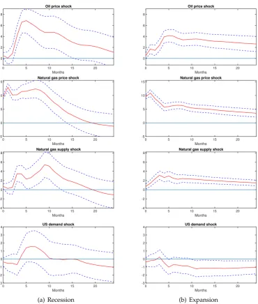
3.2 Natural gas production responses to one-standard-deviation structural shocks . . . 36

3.3 Natural gas price responses to one-standard-deviation structural shocks 37 3.4 US economy responses to one-standard-deviation structural shocks . . 37

3.5 NBER dates and weight on recession regimeF(st) . . . 39

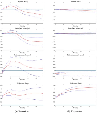
3.6 Natural gas production responses to one-standard-deviation structural shocks . . . 41

3.7 Natural gas price responses to one-standard-deviation structural shocks 42 3.8 US economic activity responses to one-standard-deviation structural shocks . . . 45

4.1 The data . . . 65

4.2 Estimated standard deviations of the structural shocks . . . 66

4.3 GIRFs for Chinese GDP growth . . . 67

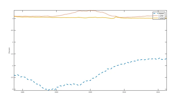
4.4 Time-varying median impact impulse responses of China’s output . . . 67

4.5 Historical decompositions of oil market variables . . . 70

4.6 GIRFs for Chinese GDP growth . . . 71

4.7 Time-varying responses of China’s output to IRAC . . . 72

4.8 Time-varying responses of China’s output to WTI . . . 72

5.1 Primary energy consumption share by fuel type (1993-2016) . . . 80

(16)

xvi LIST OF FIGURES

5.2 Evolution of the growth rate of the real price of oil, coal, natural gas

and energy. . . 83

5.3 The growth rate of Chinese energy price (by authors) and global en-ergy price (by the IMF and World Bank) . . . 85

5.4 Estimated standard deviation of the shocks . . . 94

5.5 GIRFs: Growth rate of GDP response to energy price shocks . . . 95

5.6 Median impact responses of GDP growth rate at selected horizons . . . 96

5.7 GIRFs: Inflation response to energy price shocks . . . 96

5.8 Median impact responses of inflation at selected horizons . . . 97

5.9 GIRFs: Interest rate response to energy price shocks . . . 98

5.10 GDP, inflation and interest rate responses (Chang et al. [2015]’s data) . . 98

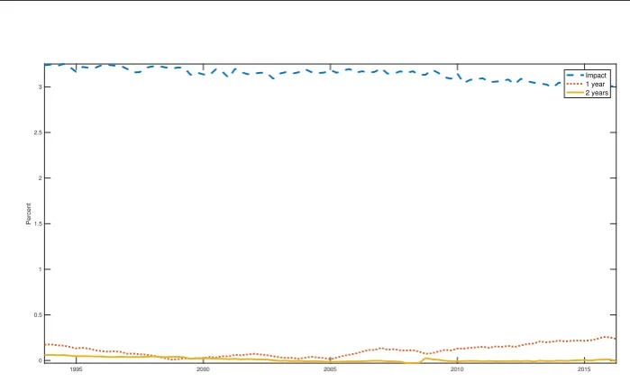
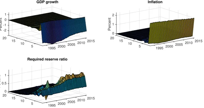
5.11 GDP, inflation and required reserve ratio responses . . . 99

5.12 GDP, CPI inflation and interest rate responses . . . 100

6.1 Share of oil, gas extraction and iron ore mining . . . 106

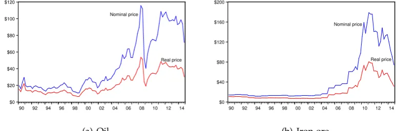
6.2 Evolution of nominal and real prices . . . 106

6.3 Impact of a 10 percent price increase driven by supply discruptions of oil and iron ore on real GDP . . . 115

6.4 Impact of a 10 percent price increase driven by supply discruptions of oil and iron ore on inflation . . . 115

6.5 Impact of a 10 percent price increase driven by supply discruptions of oil and iron ore on the interest rate . . . 116

6.6 Impact of a 10 percent price increase driven by supply discruptions of oil and iron ore on the exchange rate . . . 116

6.7 Impact of a 10 percent price increase driven by raising global demand of oil and iron ore on real GDP . . . 118

6.8 Impact of a 10 percent price increase driven by raising global demand of oil and iron ore on inflation . . . 118

6.9 Impact of a 10 percent price increase driven by raising global demand of oil and iron ore on the interest rate . . . 119

6.10 Impact of a 10 percent price increase driven by raising global demand of oil and iron ore on the exchange rate . . . 119

6.11 Impact of a 10 percent price increase driven by raising precautionary demand of oil and iron ore on real GDP . . . 121

6.12 Impact of a 10 percent price increase driven by raising precautionary demand of oil and iron ore on inflation . . . 121

(17)

LIST OF FIGURES xvii

6.14 Impact of a 10 percent price increase driven by raising precautionary

demand of oil and iron ore on the exchange rate . . . 122

6.15 Oil: historical shock decomposition of real GDP . . . 124

6.16 Iron ore: historical shock decomposition of real GDP . . . 125

6.17 Oil: historical shock decomposition of real GDP . . . 126

(18)

(19)

List of Tables

2.1 Structural changes in the US natural gas market (percent) . . . 6 2.2 Log marginal likelihood for MS-VAR(6) with different number of regimes

(Mi) . . . 15 2.3 Relative standard deviations of structural shocks by regime . . . 18

4.1 Bayes factors for competing VAR models . . . 63 4.2 Log marginal likelihood (log-ML) for competing VAR models

(numer-ical standard errors in parentheses) . . . 63 4.3 Break dates for individual equations of the baseline VAR model by the

Bai and Perron test of structural breaks . . . 64

5.1 Sign restrictions . . . 91 5.2 Log marginal likelihood (log-ML) and Bayes factor for competing VAR

models (numerical standard errors in parentheses) . . . 94

6.1 Sign restrictions for the benchmark model . . . 111 6.2 Variance decompositions: Oil vs. Iron Ore . . . 113

(20)

(21)

Chapter1

Introduction

This thesis investigates the asymmetric effects of fluctuations in a range of energy and commodity prices, including crude oil, coal, natural gas and iron ore, on macroeco-nomic activity in various economies (e.g. Australian, Chinese and the U.S.). It begins with the natural gas market (Chapter 2), in which the number of regime switches in the market is determined along with the impulse responses to structural shocks. The thesis then extends the analysis by examining the relationship between the nat-ural gas market and the price of crude oil (Chapter 3). The asymmetric reactions of US economic activity to shocks stemming from natural gas and oil market are also explored in this chapter. Next, Chapter 4 and 5 focus on the structural impacts of energy price shocks to the Chinese economy, which specially takes time-varying ef-fects into account. Finally, Chapter 6 uses the Australian economy as a case study to compare the macroeconomic impacts of crude oil and iron ore price shocks.

In order to explore the impact of energy prices on the macroeconomy, the thesis em-ploys a wide range of advanced econometric models. These models include Bayesian Vector Autoregressive (BVAR), Time varying Bayesian VAR with stochastic volatil-ity (TVP-VAR-SV), Smooth Transition VAR (ST-VAR) and Markov Switching VAR (MS-VAR). While Bayesian methods are used to improve the estimation accuracy, non-linear models are utilized to capture the possibility and significance of a time-varying and non-linear relationship between commodity price shocks and macroeco-nomic variables. Those features cannot be found in classical econometric models.

The thesis mainly extends the literature in five ways.

First, while the mentioned econometric methods have been commonly applied in mainstream macroeconomics studies that typically examine the effects of monetary and fiscal policy shocks, the use of these advanced tools to study the macroeconomic impacts of energy prices has only begun to emerge. Hence, the empirical findings

(22)

2 Introduction

in the thesis provide a better understanding of the asymmetric relationship between different energy prices and macroeconomic performance. For example, the use of the MS-VAR framework to explore regime switching in the natural gas market is novel in the literature. Similarly, using the STVAR approach to investigate the link between the natural gas and oil price and the asymmetric reactions of the US economy to energy price shocks in different phase of the business cycle is also considered as the first empirical study in the literature.

Second, not only are the advanced econometrics tools applied, but the thesis also employs a number of non standard sets of agnostic restrictions, such as sign and zero combining restrictions, sign and additional sign restrictions. These non uncon-ventional identification schemes enhance the robustness of the findings.

Third, to insure that the applied models are the best in-sample fit to the data, the thesis also conducts model comparison exercises based on marginal likelihood and Bayes factor, which is an advancement on the current literature.

Fourth, to address concerns about the quality of the Chinese macroeconomic data, the thesis compiles various data sources in the analysis, including the novel standard dataset constructed by the Federal Reserve Bank of Atlanta. The chapter based on this dataset is considered the first study using this data and has been published in Energy Economics.

Finally, one of the major contributions of the thesis is the construction of the Chinese energy price index. Since the use of oil prices as a proxy for general energy price (as in developed economies) does not extrapolate to the case of China, the thesis pro-poses a new index of primary commodity energy prices. It shows that the estimated results with the index are much more plausible and accurately reflect the structure of China’s energy expenditure shares, as well as inter-temporal fluctuations in global energy prices.

1 .

1 Thesis outline

The remainder of the thesis is organized as follows

• Chapter 2 - Understanding the US natural gas market: A Markow Switching

VAR approach.

(23)

§1.1 Thesis outline 3

activity.

• Chapter 4 - The relationship between oil price shocks and China’s output: A

time-varying analysis.

• Chapter 5 - Time varying macroeconomic effects of energy price shocks: A new

measure for China.

• Chapter 6 - Oil and iron ore price shocks: What are different economic effects

in Australia?

(24)

(25)

Chapter2

Understanding the U.S. Natural

Gas Market:

A Markov Switching VAR

Approach

2 .

1 Introduction

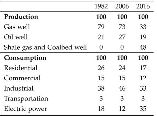
Over the past three decades, the United States (US) has witnessed significant changes in the structure of the natural gas market. These changes would not have been real-ized without a period of deregulation introduced to the market, such as the Natural Gas Wellhead Decontrol Act of 1989. Although the deregulation has often focused on price mechanisms and the supply of natural gas, but, as a results, consumers also have been affected. Indeed, decomposing the market, we can see that the changes involve both the supply and demand side, as confirmed by Table 2.1. With regard to the supply side, in the past natural gas extracted from gas wells was the primary source of gas production, accounting for 79 percent of total supplies. However, re-cently conventional form of natural gas has been replaced by unconventional forms of gas. Products found in shale gas and coalbed wells have gradually became the ma-jor source of the gas market. By 2016, unconventional gas contributed 48 percent of total natural gas production. Similarly, the significant change has also taken place on the demand side. Although commercial and residential users are still important with more than 50 percent of the market share, electric generators have, in recent years, emerged as major users, with more than one third of total natural gas consumption.

(26)

[image:26.595.153.406.126.313.2]

6 Understanding the U.S. Natural Gas Market: A Markov Switching VAR Approach

Table 2.1: Structural changes in the US natural gas market (percent)

1982 2006 2016

Production 100 100 100

Gas well 79 73 33

Oil well 21 27 19

Shale gas and Coalbed well 0 0 48

Consumption 100 100 100

Residential 26 24 17

Commercial 15 15 12

Industrial 38 46 33

Transportation 3 3 3

Electric power 18 12 35

Source: Calculation based on data from U.S. Energy Information Administration (EIA),Monthly Energy Review, various volumes.

The aforementioned change clearly suggests that the structural change is likely to exist in the US natural gas market. Therefore, in this paper I develop a multivari-ate Markov-switching (MS) model to investigmultivari-ate this structural instability of the US natural gas market over the last three decades. I makes three main contributions to the current literature. First, I conduct a formal model comparison exercise to de-termine whether there has been regime changes in the US natural gas market and how many regimes I should model to improve the model in-sample fit. Second, I investigate whether or not the detected regimes are distinct or recurrent. In other words, I investigate whether regime recurrence occurs in the US natural gas market. Third, I further investigate and compare the transmission mechanism of the regime-dependent shocks of the natural gas demand and supply to the natural gas prices in the US market.

(27)

§2.1 Introduction 7

feature of these investigations is that they do not capture the possible regime shift in the natural gas market or allow for changes in natural gas demand and production as endogenous. Brigida [2014], for example, relying on an error correction model, finds that regime-switching exists in the relationship between oil and natural gas prices but does not further investigate the underlying sources of the shift. Jadidzadeh and Serletis [2017] study the reactions of natural gas prices to shocks stemming from the global crude oil market based on a linear VAR model, which implicitly assumes that reactions of the natural gas price are time-invariant.

This paper departs from the traditional literature by proposing a Markov switching vector autoregressive (MS-VAR) model of the US natural gas market. Following the seminal work of Kilian [2009], I treat the real natural gas price as endogenous and disentangle three different types of shocks that would results from: (1) supply shocks caused by exogenous disruptions in US natural gas production; (2) demand shocks driven by unpredicted changes in US economic activity; and (3) specific demand shocks that could be associated with speculative or precautionary motives. While the specification allows for identification of the underlying shocks of the natural gas market, the MS-VAR model is an appropriate tool to detect the possible structural shift. The novelty in applying this econometric framework lies in the two main im-portant features of the MS-VAR model. First, unlike its counterparts, such as the time varying VAR model, the MS-VAR model does not restrict the size of the change when a structural break occurs but often assumes a small number of in-sample break. Hence, if the data dose not favour a large number of regimes, the MS-VAR model seems a natural choice [Sims et al., 2008]. In addition, the MS models allow for regime recurrence. This feature is not assumed in the traditional structural break models. Allowing the regime recurrence dose not only tend to improve the esti-mation accuracy but also helps us to understand more about the interrelationship among the detected regimes.

(28)

The remainder of the chapter is organized as follows: First, Section 2.2 outlines the econometric methodology, including the model specification and estimation. Next, Section 2.3 and 2.4 provide a brief overview of regulation changes and the pricing of the U.S. natural gas market and the data used in the paper. Section 2.5 then presents the results, including model comparisons, regime characteristics and im-pulse response functions. The role of oil price shocks is also examined in this section. Finally, Section 2.6 concludes the paper.

2 .

2 Empirical methodology

As highlighted in the introduction, the MS-VAR modelling framework has impor-tant features that can capture well the typical properties of the natural gas market as compared to its competitors. In general, there are three common methods that can be applied to detect the regime switching. The first method is that I can simply split the sample estimation into different subsamples and test whether there is a structural break. For example, to study the volatility of oil price shocks and the effectiveness of monetary policy, Blanchard and Gali [2008] and Nakov and Pescatori [2010] set a particular point in time (1984) as a break point. With this traditional method, we have to accept the assumption that all the parameters change at the same time, which is not necessarily the case, and more important, we should have prior knowledge of a break date, which also involves uncertainty [Boivin, 2006].

The second method is that we can utilize threshold models. These models, such as Threshold VAR or Smooth Transition VAR models, can allow for discrete shifts in parameters, like MS-VAR models, but the researcher has to specify a threshold value or transition variable.1 Recent examples of this approach in the energy literature in-clude Rahman and Serletis [2010] and Nguyen and Okimoto [2017]. Unlike threshold models, the number of regime changes detected by MS-VAR models is based on a la-tent Markov process which is directly estimated from data. In other words, the main advantage of MS-VAR models over threshold models is that the researcher needs not to predetermine the threshold value or transition variable before estimation.

Time-varying parameter models can be seen as the third framework to accommodate the nonlinearity in the relationship among the variable of interest. This modelling framework typically models variation as drifting parameters, which assumes that the

1_{Recent surveys of this literature can be found in Hubrich and Teräsvirta [2013] and Teräsvirta et al.}

(29)

§2.2 Empirical methodology 9

regime could change gradually and continuously. These models have been employed by Baumeister and Peersman [2013b], Cross and Nguyen [2017b] and Nguyen and Cross [2017] to examine the macroeconomic effects of oil and energy price shocks. Obviously, the time-varying models provide nice features that can be well suited to capturing smooth structural change of the economy. However, changes in economic structure may be not always continuous and independent. In other words, there is the possibility that changes in regime exist at a certain time. Regime changes in the natural gas market for example, due to a number of regulations and technology con-straints on production and transmission, the changes are likely discrete. In this case, the MS-VAR model can be an appropriate tool to modeling the market.

The theory and practice of MS-VAR models were laid out by Krolzig [1997] who gen-eralized the univariate MS model proposed by Hamilton [1989]. Since then, many types of the MS-VAR model have been developed and refined by Rubio-Ramirez et al. [2005]; Sims and Zha [2006]; Sims et al. [2008]; Hubrich and Tetlow [2015], Hou [2016] and Chang et al. [2017]. As with these studies, we adopt a sufficiently rich set of MS-VAR models to detect the number of regime changes in the US natural gas market and use its structure form to investigate the impacts of demand and supply shocks in the market. Specifically, coefficients and covariance shocks of the model are allowed to change over time.

In the spirit of the global crude oil model proposed by Kilian [2009], the US natural gas market is modelled by employing a three-variable MS-VAR model.2 These vari-ables include the percentage change in the US natural gas production (∆prod), the percentage change in US real economic activity (∆ip), and the percentage change in the real price of US natural gas (∆rpg). Let yt = (∆prodt,∆ipt,∆rpgt)0 be an 3×1 vector of observation at timet. The structural representation of the M-states Markov switching vector autoregressive model (MS-VAR(p)) with plag can be expressed as

B0,styt=bst+B1,styt−1+· · ·+Bp,styt−p+et, et ∼ N(0,Ωst), (2.1)

where et is assumed to independently follow a standard multivariate normal distri-bution. The reduced form of MS-VAR is obtained by premultiplying B−₀_,_s1_t to both

2_{Kilian [2009] employs the three-variable recursive VAR model consisting of global crude oil}

(30)

side of (2.1) as

yt =cst+A1,styt−1+· · ·+Ap,styt−p+et, et ∼ N(0,Σst), (2.2)

where cst is an 3×1 intercepts, A1,st, . . . ,Ap,st are 3×3 VAR coefficient matrices at

time tandN(·,·)denotes the Gaussian distribution with Σst is the 3×3 covariance

matrix . The regime indicator variable st is assumed to follow a M-state Markov process Pr(st = j|st−1 = i) = pij fori,j = 1, . . . ,M. Compactly, we can rewrite (2.2) as

yt =Xtβst+et et ∼ N(0,Σst),

where βst = vec (cst,A1,st, . . . ,Ap,st)

0

is kβ ×1 vector with kβ = 3(3p+1) and

Xt = In⊗(1,y0t−1, . . . ,y0t−p). Thus, the time-variation of the VAR coefficients (βst)

and covariance(Σ_s_t)are determined by the regime indicator variablest ∈ {1, 2, ...M}.

To complete the model specification, we assume the following independent prior for the model parameters:

βi ∼ N(β0,V0), Σi ∼ I W(S0,ν0), fori=1, . . . ,M,

whereI W(S,ν)denote the Inverse Wishart distribution with scale matrixSand the degree of freedomν. For the transition probability, we assume

(pi1, . . . ,piM)∼ D(αi1, . . . ,αiM), fori=1, . . . ,M,

where D(a1, . . . ,aM) denotes the Dirichlet distribution with concentration parame-ters (a1, . . . ,aM). This implies that the prior mean of the transition probability is given by E(pi1, . . . ,piM) = (_∑Mαi1

j=1αj1, . . . ,

αiM

∑M j=1αj1

). Generally, many time series data

evolve with high persistence, frequently switching among regimes over time is em-pirically implausible. We incorporate this feature by imposing a informative prior on the regime transition probability. To be specific, we let



    

α11 α12 . . . α1M

α21 α22 . . . α2M ..

. ... . .. ...

αM1 αM2 . . . αMM



    

=1M+ρIM,

where 1M is a M×M matrix with all its entries equal to one. The parameter ρ > 0

(31)

§2.2 Empirical methodology 11

ρ, the higher theE(pii)fori=1, . . . ,M, which implies a high regime persistence.

Identification: Having estimated the reduced form, we then recover the structural shocks of the model by assuming that each stateB0,sthas a recursive structure. There-fore, the relationship between the reduced-form error (et) and the structure shock (et), or the natural gas market fundamental shocks, in a given regime (st) can be decomposed as follows:



 

e_∆prod,t

e_∆_ip_,_t e_∆rpg,t





=



 

b11 0 0

b21 b22 0

b31 b32 b33





×



 

e_∆prod,t

e_∆ip,t

e_∆rpg,t





. (2.3)

Similar to Kilian [2009], the recursive identification scheme based on equation (2.3) postulates a vertical short-run supply curve of natural gas, which is plausible with monthly data. This assumption implies that shifts in the demand curve, either driven by US economic activity (e_∆ip) or specific factors related to the real price of natural gas (e_∆rpg) do not have a contemporaneous effect on the level of natural gas produc-tion but unexpected changes in the natural gas producproduc-tion can immediately impact on the economic activity and the price of natural gas. It also assumes that the reac-tion of US economic activity to natural gas price shocks is delayed after a month.

The impulse responses to supply and demand shocks are constructed in a given regime; we therefore ignore any feedback from changes in st into the dynamics of the natural gas market variables. By doing that, we assume the system can stay for a long time in a regime. Having said that, the estimated time-varying coefficients and variance shocks support our assumption. Results reveal that almost all regimes span a considerable length of time and hence impulse response functions in different regimes have their own economic history and can be comparable among them.

(32)

2 .

3 Regulation changes in the US natural gas market

Before estimating the model, it is useful to acknowledge the periods of important regulatory reforms in the US natural gas market. Indeed, the market received major reforms moving from a highly regulated to a highly competitive industry [Moham-madi, 2011; Joskow, 2013]. In general, over the sample period from 1980 to 2016, a major deregulation is the Natural Gas Wellhead Decontrol Act of 1989 (NGWDA) in-troduced in 1989. Therefore, the behaviour of the natural gas market can be different between periods before and after 1989.

Prior to 1989, natural gas wellhead prices were regulated by the Natural Gas Policy Act of 1978 (NGPA). The NGPA established price ceilings for wellhead first sales of natural gas that vary with the applicable gas category and gradually increase over time. It also established a three-stage elimination of price ceilings for certain cate-gories. Right after the NGPA was passed, the global crude oil market experienced a deep crisis in 1979/80, when the price of West Texas Intermediate crude oil rose from less than $15 per barrel in September 1978 to almost $40 in April 1980 [Baumeister and Kilian, 2016a]. The jump in oil prices initially exacerbated shortages of natural gas because major customers, such as industrial and electrical users, switched from oil to natural gas. However, the price of crude oil peaked only in 1981 and fell back to about $15 per barrel in July 1988, making natural gas less economical compared to crude oil. As a consequence, customers began to switch from natural gas to other forms of energy. The high volatility in oil prices and hence the large fluctuations in the demand of the natural gas market required a newly adequate price system rather than the NGPA celling price scheme introduced in 1978. As a consequence, in 1989 Congress passed the Natural Gas Wellhead Decontrol Act of 1989 (NGWDA) in an effort to bring natural gas prices up to market-clearing levels by removing all price ceilings dictated by NGPA. The US system of natural gas price regulation came to an end in 1992 with Federal Energy Regulatory Commission Order 636, further allowing more efficient use of the interstate natural gas transmission system by fundamentally changing the way pipeline companies conduct business.

2 .

4 Data

(33)

§2.4 Data 13

reviewing the pricing of natural gas in U.S. markets and then describe the data used in this paper.

As highlighted by Nguyen and Okimoto [2017], the price of gas travels from well-heads (upstream markets) where natural gas is produced to the end users (down-stream markets). According to Brown and Yucel [1993] and Mohammadi [2011], there are six separate segments, including wellhead, city gate, and four end-use nodes (e.g., commercial, industrial, residential, and electrical customers). It begins withwellhead

price. The price of gas is first determined at the wellhead by independent brokers

and pipeline companies. Therefore, the wellhead price often refers to the price of the upstream market. Pipeline companies and brokers then sell their natural gas to local distribution companies (LDCs) and some end users. The prices observed in this market refer to city gate prices. Generally, because industrial and electrical end users can switch easily between natural gas and other forms of energy to minimize their costs, these end users tend to purchase their natural gas directly from pipeline companies and brokers with competitive spot prices. For this reason, prices paid by industrial and electrical users refer to industrial pricesandelectric power prices. In contrast, commercial and residential users normally cannot switch between different fuel forms; their energy expenditure is linked with a single fuel type. As a conse-quence, both commercial customers and residential customers purchase their natural gas from LCDs, and they are offered commercial prices and residential prices, respec-tively.

The above overview suggests that, in nature, the wellhead price serves as a bench-mark reference for downstream bench-markets, including physical and spot bench-markets.3

There-fore, this paper utilizes the wellhead price as the benchmark price for the U.S. market. Similar to Jadidzadeh and Serletis [2017], we divide the nominal price series sourced from the U.S. Department of Energy (EIA) by the U.S. CPI to obtain the real price of natural gas. The natural gas price series is in percent changes by taking the first dif-ference of the monthly logarithm of the variable. We also note that the set of available data the wellhead price is only from January 1980 to December 2012. Thus, we ex-tend the data to the latest date by using natural gas import prices from January 2013 onward. That being said, because the domestic natural gas market is a competitive market, the movements of the wellhead price and the import price (in log levels) are almost identical, as can be seen from Figure 2.1. Regarding natural gas production, we use monthly U.S. natural gas gross withdrawals, also compiled by the EIA, as

3_{An examination of the relationship between upstream and downstream prices can be found in}

(34)

a proxy for natural gas supply. The variable is seasonally adjusted and then enters the model by taking the first difference of the natural logarithm. To capture the U.S. economic activity, that drives demand for natural gas in the U.S. market, we utilize the U.S. monthly industrial production index, seasonally adjusted, retrieved from the Federal Reserve Bank of St. Louis and then transform the index to a growth rate by taking the first difference of the natural logarithm. Finally, we use the US refiners’ acquisition cost for imported crude oil (IRAC), published by the EIA, to compute the real price of crude oil with the same method used to calculate for the real natural gas price.4

Figure 2.1: Historical evolution of the series (1980M2-2016M11)

Note:The shaded region shows recessions as defined by the NBER.

Figure 2.1 plots the historical evolution of our series from February 1980 to November 2016. This sample period was chosen as it is the longest set of available data for monthly US natural gas production.

2 .

5 Empirical results

We begin our analysis with a discussion of the Bayesian comparison exercise. This formal exercise is applied to determine the best model by which the number of

4_{A discussion on whether or not we should consistently use the price of oil and natural gas in}

(35)

§2.5 Empirical results 15

optimal regime changes detected. Having identified the number of regimes, we then analyse the dynamic impulse responses of the natural gas to different natural gas supply and demand shocks. The role of oil prices is also examined in this section.

2.5.1 Model comparisons

In this subsection, we conduct a formal model comparison exercise using the marginal likelihood as a selection criterion. To be specific, given model Mi, the marginal like-lihood is defined as

p(yo|Mi) =

Z

p(yo|θi,Mi)p(θi|Mi)dθi,

whereyo = (yo₁, . . . ,yo_T)is the observed data with sample size Tandθi is a vector of the parameters of model Mi. In addition, the marginal likelihood of model Mi can be rewritten as a product of one step ahead predictive likelihoods evaluated at the observed data. To be specific, p(yo|Mi) = p(yo₁|Mi)∏tT=2p(yot|y1o, . . . ,yot−1,Mi). We

will use this expression to compute the marginal likelihood and use it as a criteria determining the best candidate specification. The marginal likelihood is often used in model selection or model averaging in Bayesian data analysis. Intuitively speak-ing, the marginal likelihood can be interpreted as the predictive probability of the observed data. Thus, a larger value of marginal likelihood implies a better in-sample fit of the model given the observed data. More discussion and details about the marginal likelihood can be found in Kass and Raftery [1995].

Table 2.2: Log marginal likelihood for MS-VAR(6) with different number of regimes (Mi)

M=1 M =2 M=3 M =4 M=5

0 66.1 68.3 42.7 41.6

Note: the Table presents the relative log marginal likelihood of Mi model to the constant model (M1) model. The highest value of the log marginal likelihood

indicates the best model.

(36)

the US natural gas market. In the next subsection, we discuss the economic charac-terization of these regimes by examining the estimated coefficients and covariance shocks over time.

2.5.2 Regime characteristics

Having discovered that the 3-regime model provides the best in-sample fit for the US natural gas market, we now examine the economic characterization of these regimes. The time-varying estimated coefficients and standard deviations of the structural socks are shown in Figure 2.2 and Figure 2.3 respectively. Several interesting obser-vations arise with regard to the interpretation of these results. First, we find evidence that regime switches in the US natural gas market driven by not only the variances of shocks but also its market fundamental changes (switching in model coefficients). Therefore, the transmission of shocks is certainly different among regimes.

-2 0 2 β t,1 -0.4 -0.2 0 0.2 β t,2 -0.4 -0.2 0 0.2 0.4 β t,3 -0.05 0 0.05 β t,4 -0.1 0 0.1 β t,5 -0.2 -0.1 0 0.1 β t,6 -0.04 -0.02 0 0.02 β t,7 -0.1 0 0.1 β t,8 -0.1 0 0.1 β t,9 -0.02 0 0.02 β t,10 -0.05 0 0.05 β t,11 -0.1 0 0.1 β t,12 -0.02 0 0.02 β t,13 -0.05 0 0.05 β t,14 -0.05 0 0.05 β t,15 -0.01 0 0.01 β t,16 -0.05 0 0.05 β t,17 -0.05 0 0.05 β t,18 -0.01 0 0.01 β t,19 -1.5 -1 -0.5 0 β t,20 -0.2 -0.1 0 β t,21 0 0.2 0.4 β t,22 -0.04 -0.02 0 0.02 0.04 β t,23 -0.1 -0.05 0 0.05 β t,24 -0.1 0 0.1 0.2 β t,25 -0.02 0 0.02 β t,26 -0.04 -0.02 0 0.02 0.04 β t,27 -0.05 0 0.05 0.1 0.15 β t,28 -0.01 0 0.01 0.02 0.03 β t,29 -0.02 0 0.02 0.04 β t,30 -0.05 0 0.05 0.1 β t,31 -0.01 0 0.01 β t,32 -0.04 -0.02 0 0.02 β t,33 -0.05 0 0.05 β t,34 -0.01 0 0.01 β t,35 -0.02 0 0.02 β t,36 -0.05 0 0.05 β t,37 -10 -5 0 5

×10-3 β t,38 -4 -2 0 2 β t,39 -0.5 0 0.5 β t,40 -0.5 0 0.5 1 β t,41 -0.1 0 0.1 0.2 0.3 β t,42 -0.2 0 0.2 β t,43 -0.4 -0.2 0 0.2 0.4 β t,44 -0.2 0 0.2 β t,45 -0.2 -0.1 0 0.1 β t,46 -0.2 0 0.2 β t,47 -0.1 0 0.1 β t,48 -0.1 0 0.1 β t,49 -0.2 0 0.2 β t,50 -0.1 0 0.1 β t,51 -0.1 0 0.1 β t,52 -0.1 0 0.1 0.2 β t,53 -0.05 0 0.05 β t,54 -0.1 0 0.1 β t,55 -0.1 0 0.1 β t,56 -0.05 0 0.05 β t,57

Figure 2.2: Time-varying coefficients

Note:The figures show the estimated time-varying coefficients (βi) of MS-VAR(6) (solid lines)

together with the 95 percent probability bands (dotted lines).

Second, the results also reveal clearly that three regimes exist over the sample period from 1980M1 to 2016M11. Accordingly, a regime existed during the period before 1989, namelybefore the Decontrol Actor R1 for short. This is because this period is as-sociated with the phase that the US natural gas market was regulated by the NGPA. From 1989 onward, two different regimes are evidently detected. One regime, we

call after Decontrol Act or R2 for short, is frequently observed over the period. The

other regime prevails only in the time that the US economy was in recession, which is short lived in comparison with the other regimes. Thus, we call this is theRecession

(37)

pro-§2.5 Empirical results 17

1990 2000 2010

10 20 30 40 σ 11

1990 2000 2010

0 2 4 6 8 σ 21

1990 2000 2010

-40 -20 0

σ 31

1990 2000 2010

0 2 4 6 8 σ 12

1990 2000 2010

0.5 1 1.5 2 2.5 σ 22

1990 2000 2010

-5 0 5 10 σ 32

1990 2000 2010

-40 -20 0

σ 13

1990 2000 2010

-5 0 5 10 σ 23

1990 2000 2010

100 200 300 400 σ 33

Figure 2.3: Time varying variance - covariances

Note: The figures show the estimated time-varying covariance matrices (σi) of MS-VAR(6)

(solid lines) together with the 95 percent probability bands (dotted lines).

vides a more nuanced picture of these regimes. Following Song [2014]; Hou [2016], we plot the estimation ofP(si =sj|y1:T)and report in a table in which colour differ-ences denote different probabilities over the range of i = 1, . . . ,T and j = 1, . . . ,T. More precisely, the clustering of the regimes is presented through a T×T matrix; therefore the figure is symmetric against the 450 line. For interpretation purposes, the light color on the main diagonal of the figure indicates a new regime that occurs in the periodi= jare unique and light color off the main diagonal indicates regime recurrences. Presented in this manner, we clearly observe periods of unique regime, which confirms structure changes in the US natural gas market. At the same time, the figure also shows recurrences in regime (regime switching) existing in some pe-riods in the market.

(38)

1985 1990 1995 2000 2005 2010 2015

0 0.2 0.4 0.6 0.8 1

Figure 2.4: The estimated weighted heat map for the regime indicator (st)

Note:The figure shows the estimation ofP(si=sj|y1:T)over the range ofiand j.

Table 2.3: Relative standard deviations of structural shocks by regime

∆prod ∆ip ∆rpg

R1 1 1 1

R2 0.34 0.43 31.23 R3 4.77 2.35 57.98

Note: Entries are normalized such that the volatility of each variable is unity for the first regime (R1).

2.5.3 Regime-dependent reactions of the US natural gas market

In this subsection, I investigate the responses of the US natural gas market to its fundamental shocks and compare these responses across regimes. The market fun-damental shocks include a natural gas supply, demand and specific demand shock. We again note that, in our structural model, the supply shock presents an exogenous disruption of US natural gas production that may be caused, for example, by bad weather. This shock is normalized as a positive shock. While the demand shock arises from the fact that increases in real US economic activity, the specific demand shock is associated with specific factors, which are not directly related to the real demand for gas, causing higher natural gas prices. These factors could be associated with changes in expectation about the future price of natural gas.

(39)

Figure 2.5-2.7. Overall, the empirical results reveal that the US natural gas market is much more sensitive to its fundamental shocks occurring in Recession (R3) than other regimes. This finding is consistent with previous evidence investigated by Nguyen and Okimoto [2017] who employ a smooth transition VAR model to examine the US natural gas market. Different from my model, Nguyen and Okimoto [2017] quantify two independent regimes depending on the state of the business cycle and document that the impact of energy price shocks on US economic activity tends to be larger in recessions and than in expansions. Along with this feature, the results also reveal that the market also behaves slightly different before the Decontrol Act (R1) and after the Decontrol Act (R2) states.

5 10 15

Months 0

2 4

R1: Supply shock

5 10 15

Months 0

2 4

5 10 15

Months 0

2 4

5 10 15

Months -0.2

0 0.2 0.4

R1: Demand shock

5 10 15

Months -0.2

0 0.2 0.4

5 10 15

Months -0.2

0 0.2 0.4

5 10 15

Months -0.5

0 0.5

1 R1: Special demand shock

5 10 15

Months -0.5

0 0.5

5 10 15

Months -0.5

0 0.5

Figure 2.5: Natural gas production responses

Note:The Figures show impulse responses base on the MS-VAR(6) model of the three regimes (R1, R2 and R3). The shaded areas indicate 68% posterior credible sets.

(40)

elasticity was about inelastic under the NGPA ceiling price scheme.

5 10 15 Months

-0.5 0 0.5 1

5 10 15 Months

-0.5 0 0.5 1

5 10 15 Months

-0.5 0 0.5 1

5 10 15 Months

0 0.2 0.4 0.6

5 10 15 Months

0 0.2 0.4 0.6

5 10 15 Months

0 0.2 0.4 0.6

5 10 15 Months

0 0.2 0.4

R1: Special demand shock

5 10 15 Months

0 0.2 0.4

5 10 15 Months

0 0.2 0.4

Figure 2.6: US economic activity responses

Note:See Figure 2.5

Turning to the responses of US economic activity to natural gas supply and price shocks, I find that the economy is significantly impacted only in periods of slack economic activity, as can be seen in Figure 2.6. This evidence again confirms the finding in Nguyen and Okimoto [2017]. In particular, the results show that only the natural gas supply shock occurring before 1989 has a significant positive effect on the economy. Recently, shocks to natural gas production have a negligible impact on the US economic activity. Similarly, the economy is also found to be not very sensitive to the natural gas price shocks in normal times. This finding is contrasted with evi-dence found in the conventional literature regarding the macroeconomic impacts of crude oil price shocks on the US economy, such as Kilian [2009] and Baumeister and Peersman [2013b]. These studies find that increases in real oil prices have significant negative effect on the US economy. However, as highlighted by Nguyen and Oki-moto [2017], previous evidence often relies on linear models and ignores the fact that the macroeconomic impacts of energy price shocks may be asymmetric in different regimes. Indeed, the empirical findings in Nguyen and Okimoto [2017] indicate that in good times oil price shocks are found to be more important than natural gas price shocks. More precisely, oil price shocks have significant effects in the long run, while the natural gas price shocks have essentially no impacts on the US economy, which supports our findings.

(41)

5 10 15

Months -6

-4 -2 0

5 10 15

Months -6

-4 -2 0

5 10 15

Months -6

-4 -2 0

5 10 15

Months 0

5 10

5 10 15

Months 0

5 10

5 10 15

Months 0

5 10

5 10 15

Months 0

5 10

5 10 15

Months 0

5 10

5 10 15

Months 0

5 10

Figure 2.7: Natural gas price responses

Notes:See Figure 2.5

responses of natural gas supply and the US economy, we also observe that the dy-namic responses of the price of natural gas in the Recession regime are relatively stronger than other regimes. With regard to the impacts of the supply shock, we find a strong negative response of the natural gas price to the supply shock in the Recession regime, which is roughly 3 percent on impact. However, in response to the same shock, the effect is only 1 percent in R2 and negligible in R1. Shocks to US economic activity have negligible impact on the price of natural gas in R1 and R2 but are significant in R3. More specifically, the results reveal that, within the reces-sion regime, a one standard deviation shock to US economic activity can raise the natural gas price by about 7 percent. While shocks to natural gas production and US economic activity are found not to be the main drivers to the movements of natu-ral gas prices, impulse response results provide strong evidence that positive shocks to specific demand lead to consistent increases in the natural gas price across three regimes.

2.5.4 The role of oil prices

(42)

Figure 2.8 shows the estimated impulse response functions across three regimes.5 The results show that oil price shocks have a considerable role in influencing the natural gas price and the impact is more pronounced in recession regimes. More precisely, positive shocks to the oil price can lead to small increases in the price of natural gas but decreases in the natural gas production. The results further reveal that the strong connection between natural gas market and oil price movements only appears in recession times, in the other regimes oil price shocks have a marginal effect on natural gas quantities and prices. The results are consistent with recent findings in Nguyen and Okimoto [2017] and Caporin and Fontini [2017]. Interest-ingly, in line with previous studies, Kilian [2009], Baumeister and Peersman [2013b] for example, results obtained from the augmented model show that unexpected in-creases in the real price of oil in different regime have significantly negative effects on the US economic activity, although the effect of R2 is relative smaller. Along with these additional findings, the main results remain unchanged.

5 10 15

0 2 4 6

Oil price←Oil price shock

R1 R2 R3

5 10 15

0 0.2 0.4

Oil price←Supply shock

R1 R2 R3

5 10 15

0 0.1 0.2

Oil price←Demand shock

R1 R2 R3

5 10 15

-0.2 0 0.2 0.4 0.6 0.8

Oil price←Special demand shock

R1 R2 R3

5 10 15

-4 -2 0

NG Production←Oil price shock

R1 R2 R3

5 10 15

0 0.5 1 1.5

NG Production←Supply shock

R1 R2 R3

5 10 15

-0.05 0 0.05

NG Production←Demand shock

R1 R2 R3

5 10 15

-0.05 0 0.05 0.1 0.15

NG Production←Special demand shock

R1 R2 R3

5 10 15

-1 -0.5 0

US activity←Oil price shock

R1 R2 R3

5 10 15

0 0.2 0.4

US activity←Supply shock

R1 R2 R3

5 10 15

0 0.2 0.4 0.6

US activity←Demand shock

R1 R2 R3

5 10 15

0 0.05 0.1

US activity←Special demand shock

R1 R2 R3

5 10 15

0 2 4

NG Price←Oil price shock

R1 R2 R3

5 10 15

0 2 4 6

NG Price←Supply shock

R1 R2 R3

5 10 15

0 0.5 1 1.5

NG Price←Demand shock

R1 R2 R3

5 10 15

0 5 10

NG Price←Special demand shock

R1 R2 R3

Figure 2.8: IRFs of the augmented model

Notes:The Figures show impulse responses base on the augmented MS-VAR(6) model of the three regimes (R1, R2 and R3)

2 .

6 Conclusion

In this paper, I investigated whether regime switching exists in the US natural gas market and analysed the reactions of the market to its fundamental shocks across various regimes. To this end, I utilized a Bayesian class of MS-VAR models that

5_{To improve the readability of the plot, we do not present the error bands, but they are available}

(43)

§2.6 Conclusion 23

allows for time-variation in model coefficients and shock variances. The model en-ables us to detect efficiently the number of regime switches that are generated by both market structure change and exogenous shocks.

(44)

2 .

7 Appendix

In this Appendix we provide the MCMC algorithms for MS-VAR estimation and Priors.

2.7.1 Estimation

In this section I provide the details of the posterior sampler for MS-VAR(p). Let

Θ = {βi,Σi}_iM₌₁ be the collection of the parameters in the M regimes, and P be the

M×M Markov transition matrix, i.e., Pij = pij. To simplify the notation, we adopt the following conventionxt1:t2 = (xt1, . . . ,xt2).

The posterior draws can be obtained by sequentially sampling from:

1. p(s1:T|Θ,y1:T);

2. p(Θ|s1:T,y1:T);

3. p(P|s1:T).

To implement Step 1: I apply the forward-backward algorithm of Chib [1996]. To be specific, given p(st−1|y1:t−1,θ)we compute p(st|y1:t)by

p(st|y1:t,θ) =

p(yt|st,Θ)p(st|y1:t−1,Θ) ∑st p(yt|st,Θ)p(st|y1:t−1,Θ)

= p(yt|st,Θ)∑st−1p(st,st−1|y1:t−1,Θ)

∑stp(yt|st,Θ)p(st|y1:t−1,Θ)

= p(yt|st,Θ)∑st−1p(st|st−1)p(st−1|y1:t−1,Θ)

∑stp(yt|st,Θ)p(st|y1:t−1,Θ)

until we get p(sT|y1:T,Θ). Then we implement the backward sampling by first sam-plesT from p(sT|y1:T,Θ), then we samplestgivenst+1from

p(st|st+1:T,y1:T,Θ) =

p(st|y1:t,Θ)p(st+1|st)

∑stp(st|y1:t,Θ)p(st+1|st)

.

To implement Step 2: Note that conditionals1:T, we can regroup data into Mdistinct regimes. Fori=1, . . . ,M, the model in a regime ican be written as

yi =Xiβi+ei ei ∼ N(0,ITi ⊗Σi),

(45)

§2.7 Appendix 25

model, we have

βi ∼ N(βb_i,Kb−_i 1), Σ_i ∼ I W(bS_i,_bν_i),

where Kb_i = Xi 0

(ITi⊗Σi)

−1

Xi+V−₀1, _βb_i = Kb−_i 1

Xi

0

(ITi ⊗Σi)

−1

yi+V−₀1β0

, bνi =

Ti+ν0andbS_i = yi−Xi

yi−Xi0

+S0.

To implement Step 3: Given s1:T, we draw thejth row ofP

(p_j₁, . . . ,p_jM)∼ D(α_j₁+n_j₁, . . . ,α_jM+n_jM),

for j = 1, . . . ,M, where nkl = ∑T−_j₌₁11(sj = l,sj+1 = k) and 1(A) is the indicator

function that is equal to one if statement A is true and zeros otherwise.

To allow for convergence of the Markov chain to a stationary distribution, in all models I obtain 25,000 posterior draws, discarding the first 5,000 draws as a burn-in period.

2.7.2 Priors

I outline the hyperparameters of the prior for fitting the MS-VAR(p) model. I assume the conditional mean coefficients to follow a Minnesota prior. For the prior mean, I set β0 = 0. For the variance, I assume that V0 = diag(v1, . . . ,vk), where k =

n(np+1). If we write (v1, . . . ,vk) = vec((c0,A10, , . . . ,Ap0)0), then we setc0 to be a

vector with 10 in all its entries, i,e, the prior variance of the intercepts of the VAR model is equal to 10. For the variance of the VAR coefficient, I set

Aij_l =





 λ2₁λ2

lλ₃ σi

σj forl=1, . . . ,pandi6= j,

λ2₁

lλ₃ forl=1, . . . ,pandi= j.

(46)

(47)

Chapter3

Asymmetric Reactions of the US

Natural Gas Market and Economic

Activity

3 .

1 Introduction

A large amount of empirical literature has been devoted to understanding the be-havior of the US natural gas market, especially the relationship between the price of natural gas and crude oil. However, the literature has yet to show a consensus. Some studies, for example Pindyck [2004], Brown and Yücel [2008], Zamani [2016], and Jadidzadeh and Serletis [2017] find that movements in crude oil prices have a key role in shaping natural gas prices. In contrast, other studies conclude that there is a very weak or no connection between the two prices [Serletis and Rangel-Ruiz, 2004; Bachmeier and Griffin, 2006; Ramberg and Parsons, 2012]. In fact, empirical results obtained from these previous studies rely on linear models that assumed that the price of oil and natural gas react indifferently over the business cycle. This contrasts with recent studies emphasizing that regime-switching exists in the relationship be-tween the price of natural gas and crude oil [Brigida, 2014; Atil et al., 2014]. As a consequence, studies that do not take economic conditions into account may yield a misleading understanding about the behavior of the two energy prices.

There is also a vast literature that investigates the effects of oil prices on the real econ-omy, but there are relatively few studies that consider the effects of natural gas prices. Studies investigating the macroeconomic impacts of oil price shocks can be found in Hamilton [1983, 2003], Mork [1989], Rotemberg and Woodford [1996], Bernanke et al. [1997], Dhawan and Jeske [2008], Kilian [2009], Baumeister et al. [2010], Jo [2014],

(48)

28 Asymmetric Reactions of the US Natural Gas Market and Economic Activity

among others.1 In addition, the nonlinear relationship between energy price shocks and economic activity has recently begun to emerge in the literature. For example, while Hamilton [2003] quantifies the different effects on economic activities between oil price increases and decreases, Baumeister and Peersman [2013b] document the time-varying effects of oil supply shocks on the economy. Other studies include Huang et al. [2005], Rahman and Serletis [2011], Hamilton [2011], Katayama [2013], Baumeister and Kilian [2016b], and Cross and Nguyen [2017b]. Therefore, it is also crucial to consider possible nonlinear relationships between the energy prices and real economy.

In this chapter, we depart from the traditional literature by seeing if the US natural gas market behaves asymmetrically in different phases of the business cycle. In ad-dition, we also examine the possible asymmetry in the responses of the US economy to shocks in oil and natural gas prices. More specifically, we address the follow-ing two questions: First, are the reactions of the U.S natural gas supply and price to its market fundamental shocks different in recessions and expansions? Next, are the responses of US economic activity to oil and natural gas prices different over its business cycle? Clearly, the answer to these questions is important to understanding not only the behavior of the natural gas markets, but also the reactions of the US economy to shocks on the oil and natural gas prices in the context of a nonlinear environment, something which has not been comprehensively investigated yet in the current literature.

We address these questions by modeling an augmented natural gas market with a smooth-transition vector autoregression (STVAR) model. Following the seminal work of Kilian [2009], we model the real natural gas price as endogenous and disentangle the causes underlying market fundamental shocks. In particular, there are three fun-damental shocks stemming from the natural gas market: natural gas supply shocks, shocks to the US demand, and natural gas specific demand shocks. In addition, to account for the fact that the price of oil can influence the natural gas market as well as the US economy, we incorporate the world price of crude oil into the model and allow for shocks to the price of oil to have contemporaneous effects on the US natural gas market and economic activity. While the augmented natural gas market allows us to investigate how the US natural gas market and economic activity react to the fundamental shocks, the STVAR model provides a nonlinear framework that enables us to capture the possible state-dependent responses of the US natural gas

1_{For comprehensive surveys of the relationship between oil prices and the macroeconomy, see}

Essays in the Application of Linear and Non-Linear Bayesian VAR Models to the Macroeconomic Impacts of Energy Price Shocks